
Chapter 10
Second‐order differentials and Hessian matrices
1 INTRODUCTION
While in Chapter 9 the main tool was the first identification theorem, in this chapter it is the second identification theorem (Theorem 6.6) which plays the central role. The second identification theorem tells us how to obtain the Hessian matrix from the second differential, and the purpose of this chapter is to demonstrate how this theorem can be applied in practice.
In applications, one typically needs the first derivative of scalar, vector, and matrix functions, but one only needs the second derivative of scalar functions. This is because, in practice, second‐order derivatives typically appear in optimization problems and these are always univariate.
Very occasionally one might need the Hessian matrix of a vector function f = (fs) or of a matrix function F = (fst). There is not really a good notation and there are no useful matrix results for such ‘super‐Hessians’. The best way to handle these problems is to simply write the result as Hfs(X) or Hfst(X), that is, for each component of f or each element of F separately, and this is what we shall do; see Sections 10.9–10.11.
2 THE SECOND IDENTIFICATION TABLE
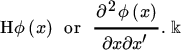
For a scalar function ϕ of an n × 1 vector x, the Hessian matrix of ϕ at x was introduced in Section 6.3 — it is the n × n matrix of second‐order partial derivatives ![]() denoted by
denoted by
We note that

The second identification theorem (Theorem 6.6) allows us to identify the Hessian matrix of a scalar function through its second differential. More precisely, it tells us that
implies and is implied by
where B may depend on x, but not on dx.
It is important to note that if the second differential is (dx)′Bdx, then H = B only when B is symmetric. If B is not symmetric, then we have to make it symmetric and we obtain H = (B + B′)/2.
If ϕ is a function of a matrix X rather than of a vector x, then we need to express dX as d vec X and write d2ϕ(X) as (d vec X)′B(d vec X). These considerations lead to Table 10.1.
Table 10.1 The second identification table
| Function | Second differential | Hessian matrix |
| ϕ(ξ) | d2ϕ = β(dξ)2 | Hϕ(ξ) = β |
| ϕ(x) | d2ϕ = (dx)′B dx | |
| ϕ(X) | d2ϕ = (d vec X)′B d vec X |
In this table, ϕ is a scalar function, ξ is a scalar, x a vector, and X a matrix; β is a scalar and B is a matrix, each of which may be a function of X, x, or ξ.
3 LINEAR AND QUADRATIC FORMS
We first present some simple examples.
4 A USEFUL THEOREM
In many cases, the second differential of a real‐valued function ϕ(X) takes one of the two forms
The following result will then prove useful.
5 THE DETERMINANT FUNCTION
Let ϕ(x) = |X|, the determinant of an n × n matrix X. We know from Section 8.3 that, at every point where X is nonsingular, the differential is given by
The second differential is therefore
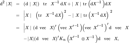
and the Hessian is

The Hessian is nonsingular if and only if the matrix ![]() . is nonsingular, that is, if and only if none of the eigenvalues of (vec In)(vec In)′ equals one. In fact, the eigenvalues of this matrix are all zero except one eigenvalue, which equals n. Hence, Hϕ(X) is nonsingular for every n ≥ 2.
. is nonsingular, that is, if and only if none of the eigenvalues of (vec In)(vec In)′ equals one. In fact, the eigenvalues of this matrix are all zero except one eigenvalue, which equals n. Hence, Hϕ(X) is nonsingular for every n ≥ 2.
Now consider the related function ϕ(X) = log |X|. At points where X has a positive determinant, we have
and hence
so that
using Theorem 10.1.
6 THE EIGENVALUE FUNCTION
If λ0 is a simple eigenvalue of a symmetric n × n matrix X0 with associated eigenvector u0, then there exists a twice differentiable ‘eigenvalue function’ λ such that λ(X0) = λ0 (see Theorem 8.9). The second differential at X0 is given in Theorem 8.11; it is

Hence, using Theorem 10.1, the Hessian matrix is
As in Section 8.9, we note that, while X0 is symmetric, the perturbations are not assumed to be symmetric. For symmetric perturbations, we have d vec X = Dnd vech(X), where Dn is the duplication matrix, and hence
using the fact that KnDn = Dn, according to Theorem 3.12.
7 OTHER EXAMPLES
Let us now provide some more examples.
8 COMPOSITE FUNCTIONS
Suppose we have two vectors x and y related through an m × n matrix A, so that y = Ax. We are interested in a scalar function ϕ(y) as a function of x.
We first consider ϕ as a function of y and define its derivative and m × m Hessian matrix:

Now we consider ϕ as a function of x. We have
and since dq = Q(y)dy,
Since the matrix A′Q(y)A is symmetric, we find

Suppose next that y (m × 1) is a function of x (n × 1), but not a linear function. This is more difficult. Writing y = f(x), we are again interested in a scalar function ϕ(y) as a function of x. We define the m × n derivative matrix A(x) = ∂f (x)/∂x′ and the n × n Hessian matrices
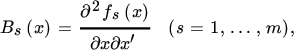
and obtain, from Theorem 6.8,

Clearly, in the linear case, the Hessian matrices Bs all vanish, so that we obtain (2) as a special case of (3).
9 THE EIGENVECTOR FUNCTION
Our Hessian matrices so far were concerned with real‐valued functions, not with vector or matrix functions. In the three remaining sections of this chapter, we shall give some examples of the Hessian matrix of vector and matrix functions.
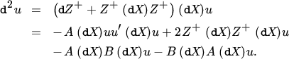
As an example of the Hessian of a vector function, we consider the eigenvector. From Theorem 8.9 we have, at points where X is a symmetric n × n matrix, dλ = u′(dX)u and du = Z+(dX)u with Z = λIn − X, and hence
Let us consider the differentials of Z and Z+, taking the symmetry of Z into account. We have
and, from Theorem 8.5,
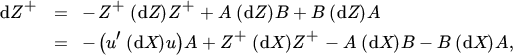
where
and we have used the facts that ZZ+ = Z+Z because of the symmetry of Z and that AB = BA = 0. This gives
To obtain the Hessian, we consider the sth component us of u. Letting es denote the vector with one in the sth position and zeros elsewhere, we obtain

and hence, from Theorem 10.1,
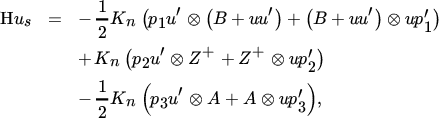
where
10 HESSIAN OF MATRIX FUNCTIONS, I
Finally, we present four examples of the Hessian of a matrix function, corresponding to the examples in Section 10.7. The first example does not involve the commutation matrix, while the other three do.
11 HESSIAN OF MATRIX FUNCTIONS, II
The next three examples involve the commutation matrix.
MISCELLANEOUS EXERCISES
- 1. Find the Hessian matrix of the function ϕ(X) = log |X′X|.
- 2. Find the Hessian matrix of the stth element Fst of the matrix function F(X) = AX−1B.
- 3. Consider the same function as in Miscellaneous Exercise 1 in Chapter 8,

where A is positive definite and X has full column rank. Show that
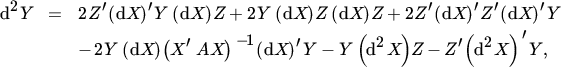
where

If Y is considered as a function of X, then d2X = 0. However, if X in turn depends on a vector, say θ, then dX and d2X need to be expressed in terms of dθ.