In Chapter 13, we considered the simple linear regression model
(1)
where yt and ut are scalar random variables and xt and β0 are k × 1 vectors. In Section 15.8, we generalized (1) to the multivariate linear regression model
(2)
where yt and ut are random m × 1 vectors, xt is a k × 1 vector, and B0 a k × m matrix.
In this chapter, we consider a further generalization, where the model is specified by
(3)
This model is known as the simultaneous equations model.
2 THE SIMULTANEOUS EQUATIONS MODEL
Thus, let economic theory specify a set of economic relations of the form
(4)
where yt is an m × 1 vector of observed endogenous variables, xt is a k × 1 vector of observed exogenous (nonstochastic) variables, and u0t is an m × 1 vector of unobserved random disturbances. The m × m matrix Γ0 and the k × m matrix B0 are unknown parameter matrices. We shall make the following assumption.
Given the nonsingularity of Γ0, we may postmultiply ( 4
) with , thus obtaining the reduced form
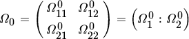
It is clear that the vectors {v0t, t = 1, …, n} are independent and identically distributed as N(0, Ω0), where . The loglikelihood function expressed in terms of the reduced‐form parameters (Π, Ω) follows from Equation (19) in Chapter 15:
(7)
where
Rewriting (7) in terms of (B, Γ, Σ), using Π = −BΓ−1 and Ω = Γ−1′ΣΓ−1, we obtain
(8)
where
The essential feature of (8) is the presence of the Jacobian term of the transformation from ut to yt.
There are two problems relating to the simultaneous equations model: the identification problem and the estimation problem. We shall discuss the identification problem first.
Exercise
1.
1.
In Equation ( 8
), we write rather than log |Γ|. Why?
3 THE IDENTIFICATION PROBLEM
It is clear that knowledge of the structural parameters (B0, Γ0, Σ0) implies knowledge of the reduced‐form parameters (Π0, Ω0), but that the converse is not true. It is also clear that a nonsingular transformation of ( 4
), say
leads to the same loglikelihood ( 8
) and the same reduced‐form parameters (Π0, Ω0). We say that (B0, Γ0, Σ0) and (B0G, Γ0G, G′Σ0G) are observationally equivalent, and that therefore (B0, Γ0, Σ0) is not identified. The following definition makes these concepts precise.
4 IDENTIFICATION WITH LINEAR CONSTRAINTS ON B AND Γ ONLY
In this section, we shall assume that all prior information is in the form of linear restrictions on B and Γ, apart from the symmetry constraint on Σ.
5 IDENTIFICATION WITH LINEAR CONSTRAINTS ON B, Γ, AND Σ
In Theorem 16.2 we obtained a global result, but this is only possible if the constraint functions are linear in B and Γ and independent of Σ. The reason is that, even with linear constraints on B, Γ, and Σ, our problem becomes one of solving a system of nonlinear equations, for which in general only local results can be obtained.
6 NONLINEAR CONSTRAINTS
Exactly the same techniques as used in establishing Theorem 16.3 (linear constraints) enable us to establish Theorem 16.4 (nonlinear constraints).
7 FIML: THE INFORMATION MATRIX (GENERAL CASE)
We now turn to the problem of estimating simultaneous equations models, assuming that sufficient restrictions are present for identification. Maximum likelihood estimation of the structural parameters (B0, Γ0, Σ0) calls for maximization of the loglikelihood function ( 8
) subject to the a priori and identifying constraints. This method of estimation is known as full‐information maximum likelihood (FIML). Finding the FIML estimates involves nonlinear optimization and can be computationally burdensome. We shall first find the information matrix for the rather general case, where every element of B, Γ, and Σ can be expressed as a known function of some parameter vector θ.
8 FIML: ASYMPTOTIC VARIANCE MATRIX (SPECIAL CASE)
Theorem 16.5 provides us with the information matrix of the FIML estimator , assuming that B, Γ, and Σ can all be expressed as (nonlinear) functions of a parameter vector θ. Our real interest, however, lies not so much in the information matrix as in the inverse of its limit, known as the asymptotic variance matrix. To make further progress we need to assume more about the functions B, Γ, and Σ. Therefore, we shall assume that B and Γ depend on some parameter, say ζ, functionally independent of vech(Σ). If Σ is also constrained, say Σ = Σ(σ), where σ and ζ are independent, the results are less appealing (see Exercise 3).
Exercises
1.
1.
In the special case of Theorem 16.6 where Γ0 is a known matrix of constants and B = B(ζ), show that the asymptotic variance matrix of and vech is
2.
2.
How does this result relate to the expression for ℱ−1 in Theorem 15.4.
3.
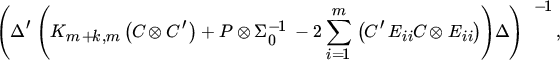
Assume, in addition to the setup of Theorem 16.6, that Σ is diagonal and let σ be the m × 1 vector of its diagonal elements. Obtain the asymptotic variance matrix of . In particular, show that , the asymptotic variance matrix of , equals
where Eii denotes the m × m matrix with a one in the ith diagonal position and zeros elsewhere.
9 LIML: FIRST‐ORDER CONDITIONS
In contrast to the FIML method of estimation, the limited‐information maximum likelihood (LIML) method estimates the parameters of a single structural equation, say the first, subject only to those constraints that involve the coefficients of the equation being estimated. We shall only consider the standard case where all constraints are of the exclusion type. Then LIML can be represented as a special case of FIML where every equation (apart from the first) is just identified. Thus, we write
(42)
(43)
The matrices Π01 and Π02 are unrestricted. The LIML estimates of β0 and γ0 in Equation (42) are then defined as the ML estimates of β0 and γ0 in the system ( 42
)–(43).
We shall first obtain the first‐order conditions.
10 LIML: INFORMATION MATRIX
Having obtained the first‐order conditions for LIML estimation, we proceed to derive the information matrix.
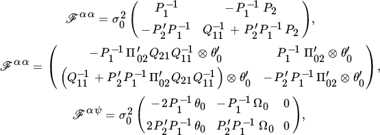
11 LIML: ASYMPTOTIC VARIANCE MATRIX
Again, the derivation of the information matrix in Theorem 16.8 is only an intermediary result. Our real interest lies in the asymptotic variance matrix, which we shall now derive.
3.
3.
Let . What is the interpretation of the hypothesis θ02 = 0?
4.
Show that
where
is partitioned conformably to θ0 (see Smith 1985). How would you test the hypothesis θ02 = 0?
5. Show that H* in Theorem 16.9 is positive semidefinite.
6. Hence show that
BIBLIOGRAPHICAL NOTES
3–6. The identification problem is thoroughly discussed by Fisher (1966). See also Koopmans, Rubin, and Leipnik (1950), Malinvaud (1966, Chapter 18), and Rothenberg (1971). The remark in Section 16.5 is based on Theorem 5. A.2 in Fisher (1966). See also Hsiao (1983).
7–8. See also Koopmans, Rubin, and Leipnik (1950) and Rothenberg and Leenders (1964).
9. The fact that LIML can be represented as a special case of FIML where every equation (apart from the first) is just identified is discussed by Godfrey and Wickens (1982). LIML is also close to instrumental variable estimation; see Kleibergen and Zivot (2003) for relationships between certain Bayesian and classical approaches to instrumental variable regression.
10–11. See Smith (1985) and Holly and Magnus (1988).

 rather than log |Γ|. Why?
 and vech
  is
is

 . In particular, show that
  , the asymptotic variance matrix of
  , equals


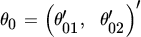 . What is the interpretation of the hypothesis θ02 = 0?