
3
Uncertainty
This chapter focuses on uncertainty and the means to evaluate it through a mathematical theory of probability. Our objective here is to pedagogically present such a theory as a way to operate with random variables and random processes with special attention to well‐defined systems following the demarcation process presented in Chapter 2. In this case, uncertainty can be related to either internal or external aspects of a given particular system, as well as to its articulation with its environment. We will introduce this theoretical field in an accessible manner with an explicit intention of reinforcing foundational concepts instead of detailing mathematical techniques and derivations. Such concepts are the raw material needed to understand the definition of information to be presented in Chapter 4. For readers with interest in the mathematics, the original book by Kolmogorov is a must [1]. Engineers and engineering students could also refer to [2] and readers with interest in complex systems to [3].
3.1 Introduction
The word “uncertainty” refers to aspects of a phenomenon, an object, a process, or a system that are totally or partly unknown, either in relative or absolute terms. For example, it is uncertain to me how many people will read this book, or if I will be able to travel to Brazil in the summer vacations. It is also uncertain to me who will win the lottery this evening; however, I am certain that I will not win because I have no ticket. Other phenomena involve even more fundamental types of uncertainty as, for instance, quantum mechanics (e.g. Heisenberg's uncertainty principle) or chaotic systems that are sensitive to initial conditions that are impossible to determine with the required infinite precision.
Probability theory is a branch of mathematics that formalizes the study of uncertainty through a mathematical characterization of random variables and random processes. Its basis is set theory, and it is considered to have been inaugurated as an autonomous field when Kolmogorov postulated the axioms of probability theory [1]. We can affirm that probability theory is a purely theoretical discipline related to purified mathematical objects. To avoid misunderstanding, it is worth mentioning that the treatment of uncertainty in real‐world data is related to another discipline called statistics. While statistics is, in fact, founded on probability theory, it constitutes an autonomous technical discipline based on its own methodology and raw materials. Interestingly, the ongoing research efforts in machine learning and artificial intelligence are closely related to statistics and hence, probability theory. Some aspects of statistics will be discussed in forthcoming chapters.
Our focus here is only on the fundamentals of probability theory. We will mostly provide some intuitive concrete examples as illustrations, which are controlled experimental systems isolated from the environment (i.e. a closed system), and thus, a rigorous analysis of real‐world data is put aside. In this sense, the most important concepts and the basics of their mathematical formulation will be stated in a comprehensive manner.
3.2 Games and Uncertainty
Most games involve some sort of randomness. Lottery, dices, urns, roulette, or even simple coin flipping are classical examples of games that are almost entirely a chance game. Those are usually one‐shot games, and the uncertainty is directly related to the outcome in relation to choices the players have taken before the outcome is revealed. They are usual examples in probability theory textbooks.
Other classes of games, like chess or checkers, are strategic and, in some sense, deterministic. However, the (strategic) interactions between the two players in order to win also lead to uncertainty but of a different type in comparison with chance games. We can say that this is more an operational uncertainty in a sense that it is impossible to know with certainty how the process will evolve, except in very few (unrealistic) cases where very strong assumptions about the players are taken (e.g. both players will always act in the same way when faced with the same situation).
There are other kinds of games that combine both types of uncertainty. These are games where the initial state of the players is given by a drawing process (like a lottery), and the game itself is based on (strategic) decisions of players. Card games and dominoes are well‐known examples. These are the most interesting games to exemplify and introduce the idea of random variables and random processes. Because of its relative simplicity, our discussions will mainly concern dominoes, whose main aspects will be defined next. Note that all games considered in this chapter are closed systems.
A full set of dominoes is shown in Figure 3.1a, while a snapshot of a typical deck is presented in Figure 3.1b. This game is interesting because it provides a pedagogical way to present probability theory, ranging from the simplest case of one random variable to the most challenging cases of random processes. In more precise terms, there are two main sources of uncertainty in dominoes, namely (i) the drawing processes at the beginning and during the game, and (ii) the behavior of the players, who are dynamically interacting in a sequential process. In this case, interesting questions could be posed: (a) how frequently will a player begin with the same hand; (b) how frequently will all players begin with the same hand; and (c) how frequently will a game with all players starting with the same hand lead to the same playing sequence resulting in identical games? Without any formalism, even a child can readily answer that (a) is more frequent than (b) and (c), and (b) more frequent than (c). Our task is then not only to prove these inequalities but also to find a way to quantify the chances of these outcomes. Let us move step‐by‐step in a series of examples.
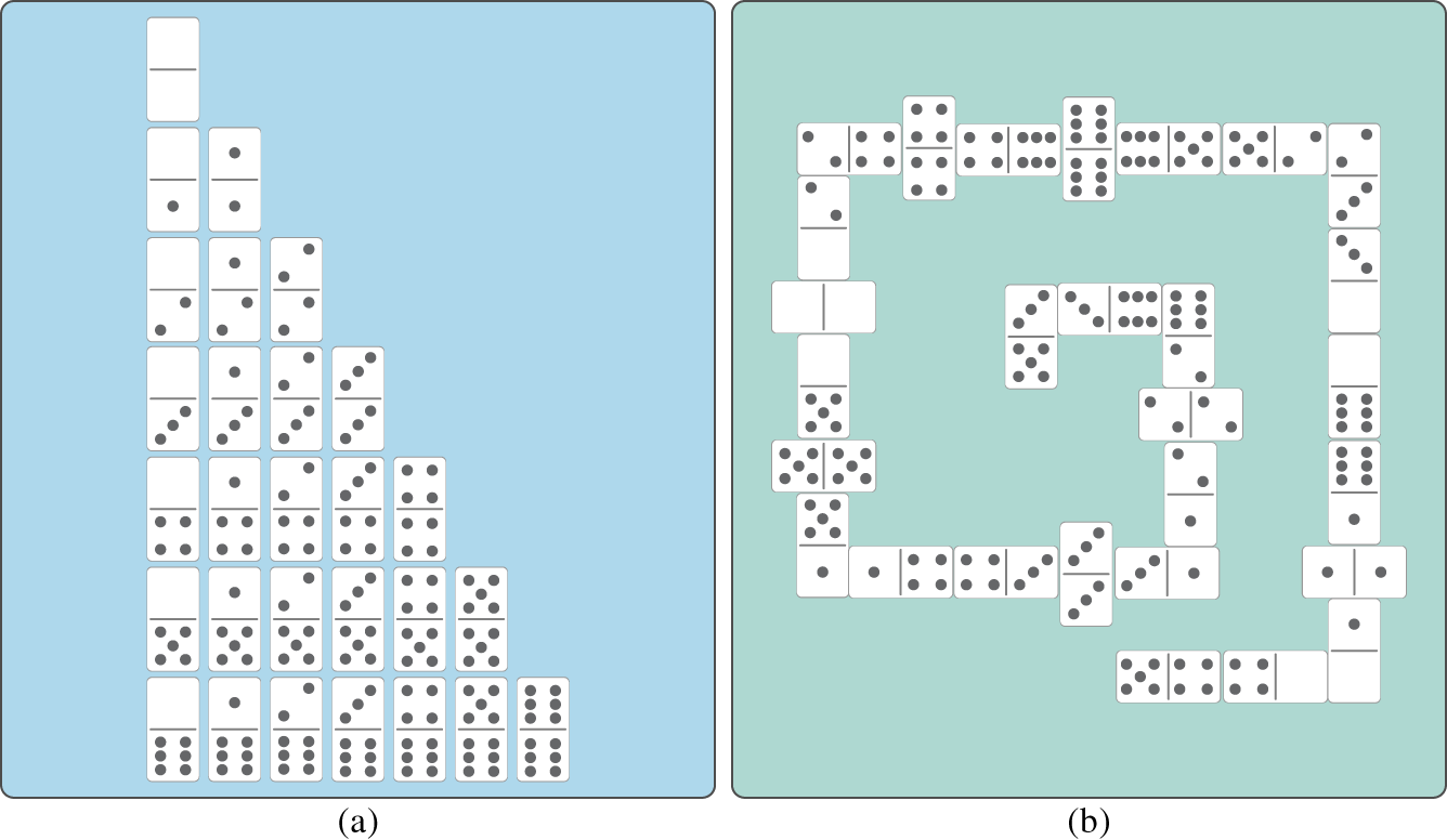
Figure 3.1 (a) Dominoes set; (b) example of a game.
Now, we can provide an outline of how to answer the three questions posed before these four examples. For the question (a) how frequently will a player begin with the same hand, we should proceed similar to Example 3.3 but indicating the order in which the pieces are taken from the deck (i.e. whether the player is the first one to take the five tiles, or if there is a different procedure for taking the tiles). The idea is to check the favorable outcomes (the specific five tiles) with respect to the number of pieces in the deck. The question (b) how frequently will all players begin with the same hand follows the same procedure, but each player has to be analyzed individually, and all players must have the same five tiles. However, it is easy to see that the situation described in (a) is completely covered by the situation in (b), which specifies even further the favorable outcome. We can say that the favorable outcome related to (a) is a subset of the one described in (b). For being more restrictive, the chances of (b) are smaller than (a).
The last question (c) how frequently will a game with all players starting with the same hand lead to the same playing sequence becoming identical games is trickier. First, the situation described in (b) is covered by the one described in (c), and thus, (c) has, at best, the same chance as (b). However, (c) involves an operational uncertainty related to how the game develops from the decisions and actions of the (strategic) players. Such decision‐making processes are, in principle, unknown, and thus, we cannot compute the chances related to them without imposing (strong) assumptions. For example, if we assume that (i) all players will always take the same decisions and actions when they are in the same situation, and (ii) they play in the same sequence, then if they have the same tiles, the outcome of the game will be the same, reducing the chances of (c) happening to the outcome that all players have the same hands, which is the situation described in (b). In this case, the chances of (b) and (c) are the same. Nevertheless, any other assumption related to the players' behavior would imply more possibilities and therefore, the chances of (c) to occur would be lower than (b), and thus, (a). The situation described in (a) and (b) refers to random variables, while (c) refers to random processes or stochastic processes. Random variables are then associated with single observations, while stochastic processes with sequential observations constituted by indexed (e.g. time‐ or event‐stamped) random variables considering the order of the observations. More details can be found in [3].
Besides, an attentive reader will probably not be satisfied because the questions talk about the frequency of a specific outcome and the answers displace the question of talking about the chances of those outcomes. This is a correct concern. The fundamental fact taken into account in those cases is that the studied outcomes are one‐shot realizations of either a given process of drawing as in (a) and (b), or of a well‐determined dominoes complete match as in (c). Since each one‐shot realization of the process is unrelated to both previous and future realizations, the outcomes are then independent. A deeper discussion about the dependence and independence of outcomes will be provided later in this chapter. Let us now exemplify this by revisiting Example 3.1.
With this example, we have shown that the frequency of the outcomes in a (fair) drawing process can be approximated by the chance of a given outcome in a one‐shot realization. If the drawing process is repeated many many times, then the frequency will tend to have the same value as the chance of a one‐shot realization. For the questions asked in (a), (b), and (c), this fact is enough to sustain that frequency and chance have the same numerical value. But we need to go further, and this will require some formalization of the concepts presented so far in order to extend them. In the following section, we will start our quick travel across the probability theory world always trying to provide concrete examples.
3.3 Uncertainty and Probability Theory
Consider a particular system or process containing different observable attributes that can be unambiguously defined. For example, the dominoes set has 28 tiles with two numbers between zero and six, coins have two sides (heads and tails), the weather outside can be rainy or not, or the temperature outside my apartment during July could be any temperature between ![]() 10 and 35
10 and 35 ![]() C. Given these observations, there is an unlimited number of possible experiments that could be proposed. One experiment could be related to measuring the temperature outside for the whole July, every day at 7 am and 7 pm. Another experiment could be to throw a coin five times in a row and then record the sequence of heads and tails. The examples provided with dominoes in the previous sections are all different experiments related to drawing tiles of the dominoes set.
C. Given these observations, there is an unlimited number of possible experiments that could be proposed. One experiment could be related to measuring the temperature outside for the whole July, every day at 7 am and 7 pm. Another experiment could be to throw a coin five times in a row and then record the sequence of heads and tails. The examples provided with dominoes in the previous sections are all different experiments related to drawing tiles of the dominoes set.
Each experiment is thus defined by events related to observations of a set of predefined attributes of the system following a well‐defined protocol of action (i.e. a procedure of how to observe and record observations). Depending on the specific case, the result of an observation is referred to as outcome, sample, measurement, or realization. If, before the observation, the attribute to be observed has its outcome already known with certainty, the system or process is called deterministic. If this is not the case, there is uncertainty involved, and thus, the possible set of outcomes is associated with chance, or probability.
The formal notation to be employed here will be presented next.
It is noteworthy that the proposed notation formalizes the observation process with respect to a system or process. This is a remarkable difference from most textbooks, e.g. [2], where neither the observation protocol grounded in a particular system or process is formalized nor its randomness is formally defined with respect to the experiment under consideration. Although these aspects are found in most books in a practical state, our aim here is to explicitly formalize them in order to support the assessment and evaluation of the uncertainty of different systems and processes. To do so, we first need to mathematically define probability measure.
These are the well‐known axioms of probability proposed by Kolmogorov [1]. In plain words: probability is positive with a maximum value of 1, where the probability of two disjoint sets is the sum of their individual probabilities. With those three basic axioms, it is possible to derive several properties of ![]() [1, 2].
[1, 2].
With Definitions 3.2 and 3.3, we can return to the dominoes but now discussing probabilities.
What is interesting is that one can propose an unlimited number of experiments following the same basic observation process related to a particular system. In this case, it is also important to have a more detailed characterization of it, which can then be used to solve questions related to different experiments grounded in that process. One important tool is the frequency diagrams or histograms. The idea is quite simple: repeat the observation process several times, counting how many times each attribute is observed, and then plot it with a bar diagram associating each attribute with its respective number of observations. Figure 3.2 illustrates this for the case of the dominoes set.
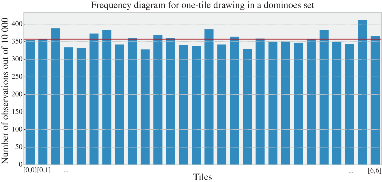
Figure 3.2 Example of a frequency diagram related to the observations of the attributes  (two numbers in the tile) of the system
  (a dominoes set composed of 28 tiles) following the observation protocol
  repeated for 10 000 times. The dark gray line indicates the expected number of occurrences for each tile.
In this case, the dark gray line is the expected number of occurrences of each tile; this number is intuitively defined as the probability of a given outcome (in this case 1/28) times the number of observations (in this case 10 000). This leads to an expected number of 357.14 observations for each different tile. Let us try to better understand this with the following examples.
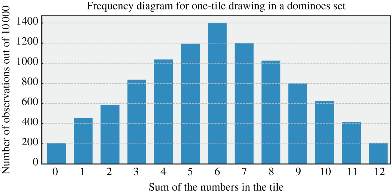
Figure 3.5 Example of a frequency diagram related to the attribute 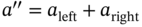 with
with 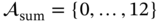 of the system
  (dominoes set composed of 28 tiles) following the observation protocol
  repeated for 10 000 times.
With these examples, we have shown how the different observation protocols define the observable outcomes and the respective sample spaces, which are the basis of specific experiments constructed to evaluate the uncertainty of particular systems or processes. Because the values of the attributes may vary at every observation, it is then possible to create a map that associates each possible observable attribute with a probability that it will be indeed observed as the outcome of one observation. Probability theory names a quantified version of this unknown observable attribute as random variable and the mathematical relation that maps the random variable with probabilities as probability functions; they are formally defined in the following.
This can now be used not only to better characterize the uncertainty related to different processes and systems but also to develop a whole mathematical theory of probability. From the probability function, it is also possible to define a simpler characterization of random variables. For example, it is possible to indicate which is the outcome that is more frequent, or the average value of outcomes, or how much the outcomes vary. Among different possible measures, we will define next the moments of random variables, which can be directly employed to quantify their expected value and variance.
Besides, it is worth introducing two other concepts that are helpful to analyze different observation processes. Consider a case of different observations of the same random variable ![]() (i.e. all conditions of the observation process are the same). If a given observation of this process does not depend on past and future observations, we say that the realizations of
(i.e. all conditions of the observation process are the same). If a given observation of this process does not depend on past and future observations, we say that the realizations of ![]() are independent and identically distributed (iid), which will lead to a memoryless process (a formal definition will be provided later). We can now illustrate these concepts with some examples.
are independent and identically distributed (iid), which will lead to a memoryless process (a formal definition will be provided later). We can now illustrate these concepts with some examples.
In this example, although it is possible to compute the expected value and the variance, these measures are meaningless because the mapping function ![]() is arbitrary and its actual values are not related to the attribute
is arbitrary and its actual values are not related to the attribute ![]() . Note that, in other cases, the mapping is straightforward from the measurement as, for instance, the number of persons in a queue. In summary, the correct approach to define the random variable under investigation depends on the system or process
. Note that, in other cases, the mapping is straightforward from the measurement as, for instance, the number of persons in a queue. In summary, the correct approach to define the random variable under investigation depends on the system or process ![]() , the observation protocol
, the observation protocol ![]() , and the experiment
, and the experiment ![]() of interest.
of interest.
It is also important to mention that one interesting way to numerically estimate probability mass functions is by experiments like the ones presented in Figures 3.2, 3.4, and 3.5. Those results were obtained by computer simulations based on the Monte Carlo method [4]. The idea is to generate several observations and empirically find their probabilities as the number of times that a specific observation appears divided by the overall number of observations realized. Figure 3.6 presents analytical results generated from the probability mass function ![]() for
for ![]() and empirical results generated by computer simulations. Note that this random variable is uniformly distributed in relation to its sample space.
and empirical results generated by computer simulations. Note that this random variable is uniformly distributed in relation to its sample space.
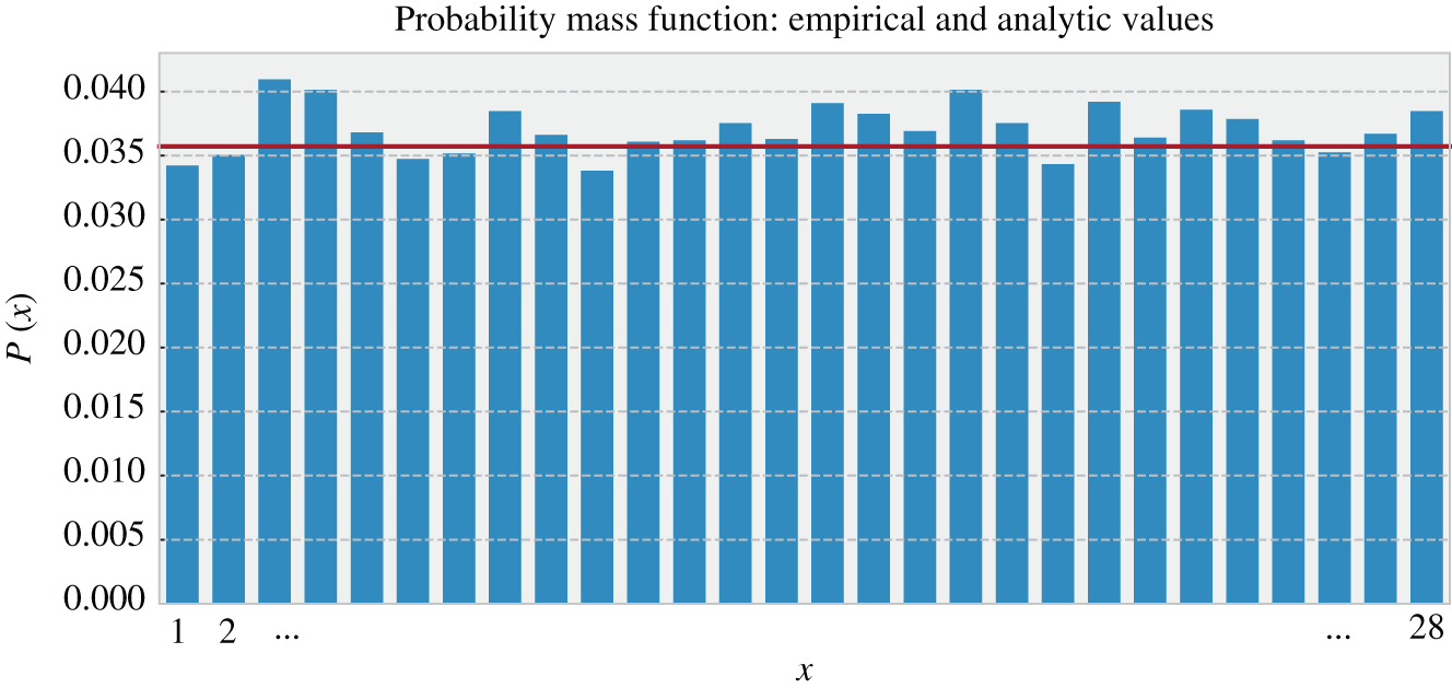
Figure 3.6 Example of a probability mass function diagram related to the random variable  obtained from the observations of the attributes
  (two numbers in the tile) of the system
  (dominoes set composed of 28 tiles) following the observation protocol
  repeated for 10 000 times. The bars are the empirical results, and the line indicates the analytic probabilities.
As a matter of fact, there are several already named probability distributions, for instance, Gaussian or Normal distribution, Poisson distribution, and Binomial distribution. Their mathematical characterization is available in different public repositories and textbooks, e.g. [2].
The importance of having a well‐defined formulation of probability distributions is to perform computer experiments in a generative manner. The idea is to describe a real‐world process or system with a known probability distribution and simulate its dynamics. Note also that, in many cases, the random variable values can be directly obtained from observations of the attributes, without defining a special mapping function as in Example 3.8.
Most of the examples presented in this section illustrate experiments where the different observations of the specific random variables are assumed iid. However, this is not always the case. Example 3.7 shows one type of dependence, because there is one new random variable defined as the sum of two other random variables. Another example is a drawing process presented in Example 3.1 but without returning the observed tile to the bank, which decreases the sample space, and thus, modifies the probability distribution. There are many other modes of dependence between two or more random variables, which include operations and functions of random variables, and random processes. These topics will be the focus of our next section.
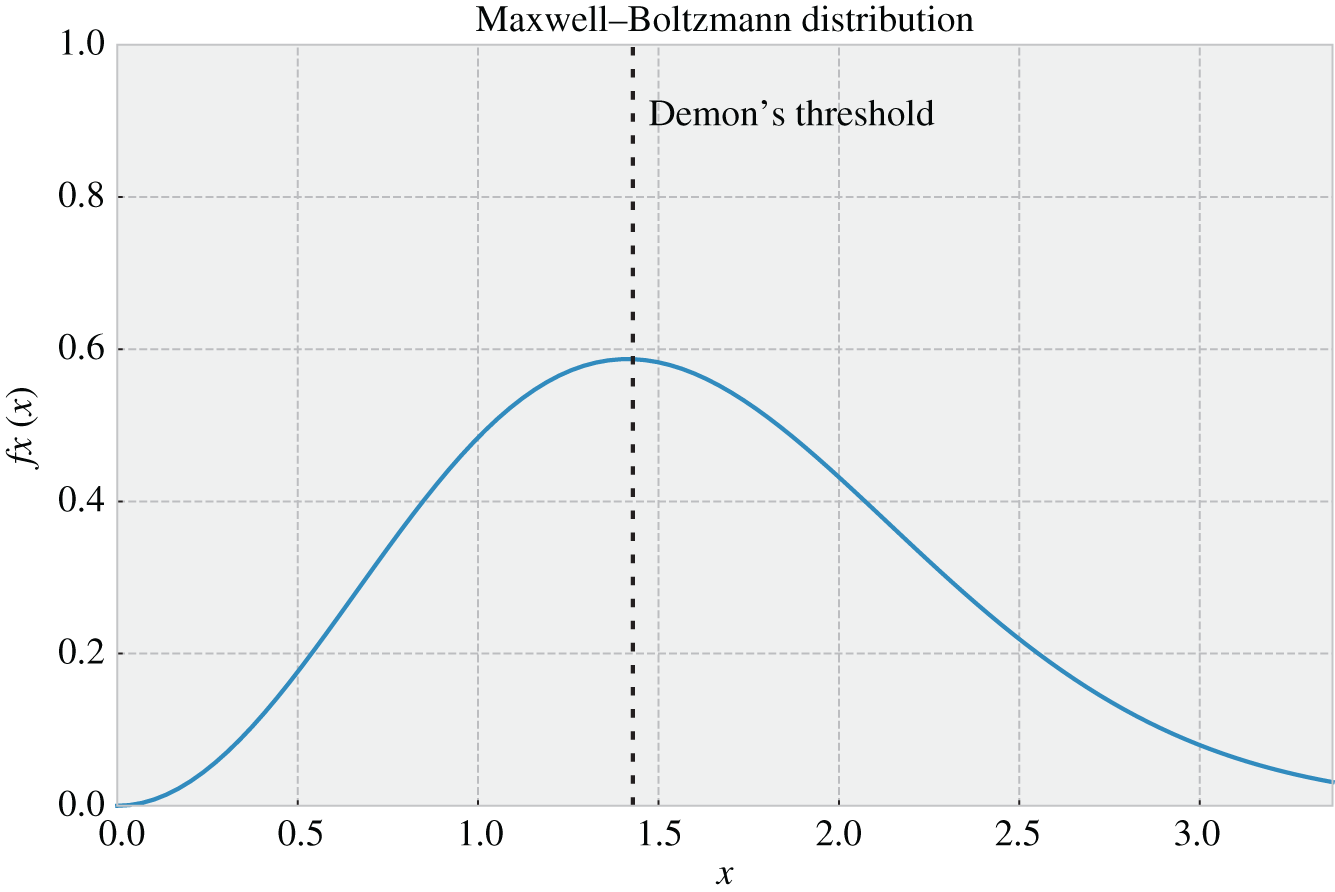
Figure 3.8 Maxwell–Boltzmann probability density function of the random variable that characterizes the speed of the gas molecules for  (arbitrary value) indicating the separation threshold used by Maxwell's demon to separate the fast and slow molecules.
3.4 Random Variables: Dependence and Stochastic Processes
When thinking about systems and processes, we intuitively imagine that different observations of attributes and outcomes of experiments may be dependent. Observable attributes might be related to a background process or system, for example, when measuring temperature in a room using two sensors in different places, or the same sensor but whose measurements are taken every ten minutes. In both cases, if we consider that these observable attributes are associated with random variables, it is expected that they would be related to each other as they are measurements of the temperature (a physical property) of the same place. Hence, if the outcome of one of these random variables is known, the uncertainty of the other should decrease.
In other cases, the attributes might have another type of physical dependence, like the rotation speed of rotors in electric machines and the associated values of electric current and voltage. There is also the case of relations that are constructed in the design of the experiment of interest. For instance, in Example 3.7, the outcome of the experiment is constructed as the sum of two attributes that are characterized as two independent random variables.
Another type of dependence between random variables is related to sequential processes as exemplified by a dominoes game where the sample space dynamically changes at each action. A queue at the cashier of a supermarket also illustrates a sequential process where the number of persons waiting in the line to be served depends on the number of persons arriving in the queue and the service time that each person requires to leave the cashier.
To evaluate the dependence between random variables, it is necessary to formally define a few key concepts, as to be presented next.
To mathematically characterize the dependence/independence of random variables, we need to consider functions of two or more random variables. They are the joint, conditional, and marginal probabilities distributions. Therefrom, it is possible to propose a classification of types of uncertainties associated with different systems, processes, and experiments. Their formal definition is provided next.
Despite the potentially heavy mathematical notation, the concepts represented by those definitions are quite straightforward. The following example illustrates the key ideas.
Another possible way to create a dependence is by defining experiments where new random variables are defined as functions of already defined ones. For example, one new random variable can be a sum or a product of two other random variables. Example 3.7 intuitively introduces this idea. Despite the importance of this topic, the mathematical formulation is rather complicated, going beyond the introductory nature of this chapter. The reader can learn more about those topics, for example, in [2]. What is extremely important to remember is that one shall not manipulate random variables by usual algebraic manipulation; random variables must be manipulated according to probability theory.
Before closing this chapter, there is still one last topic: stochastic processes. A stochastic process, also called random process, is defined as a collection of random variables that are uniquely indexed by another set. For instance, this index set could be related to a timestamp. If we consider that the temperature measured by a given thermometer is a random variable, the index set can be a specific timestamp (i.e. year‐day‐hour‐minute‐second) of the measurement. The stochastic process is then a collection of single measurements – which is the random variable – indexed by the timestamp. A formal definition is presented next.
The different observations that form a stochastic process can be composed of iid random variables as in Example 3.5. However, this is not always the case, and thus, it is important to define random processes in terms of how a given observation is related to past observations of the same process. We will follow [3] and define the following types of stochastic processes.
This ends the proposed brief review of probability theory. Now that we are better equipped to mathematically characterize uncertainty in processes and systems, we can move on to the next chapter, where we will define information as a concept that indicates uncertainty resolution.
3.5 Summary
This chapter introduced the mathematical theory of probability as a formal way to approach uncertainty in systems or processes. By using intuitive examples, we navigated through different concepts like observation process, random variables, sample space, and probability function, among others. The idea was to set the basis for understanding the cyber domain of cyber‐physical systems, which is built upon information – a concept closely associated with uncertainty. As a final note, we would like to stress that the present chapter is an extremely brief introduction, and thus, interested readers are strongly suggested to textbooks in the field, such as [2]. Another interesting book is [3], where the authors build a theory for complex systems using many fundamental concepts of probability theory. In particular, its second chapter provides a pedagogical way to characterize random variables and processes, including well‐known probability distributions and stochastic processes. Finally, reading the original work by Kolmogorov [1] may be also a beneficial exercise.
Exercises
- 3.1 Players drawing two times the same five tiles. Example 3.3 analyzed the situation where one player is the first one to get five tiles out of the full set containing 28 tiles. The task here is to evaluate other situations.
- Compute the chances of the player to get the same five tiles considering that he/she draws after the first one has drawn his/her five tiles.
- Consider that the drawing is performed in a sequential manner so that one player gets one tile first, then the other player gets the second tile, and so on. Compute the chances of the first player of the sequence of getting the same five tiles regardless of the other player's hand.
- Compute the chances of the second player of the sequence of getting the same five tiles regardless of the other player's hand.
- Consider the situation where both players get the same hand. Does the drawing protocol affect the chances of the outcome?
- 3.2 Formal analysis to compute probability. The task in this exercise is to practice the formalization proposed in Definitions 3.2 and 3.3 and illustrated in Example 3.5.
- Formalize the results obtained in Example 3.2, computing the probability associated with the events described there.
- Do the same for Example 3.3.
- 3.3 Maxwell's demon operation. Consider Example 3.10. The task is to formalize the Maxwell's demon experiment based on probability theory and illustrate the equilibrium macrostates before and after the demon's intervention.
- Formalize the experiment following Definitions 3.2 and 3.3.
- Plot the Maxwell–Boltzmann distribution introduced in (3.7) for
 , which is the equilibrium state before the demon's intervention.
 - Find the separation threshold value
 that leads to
 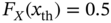 .
. - Plot an estimation of the Maxwell–Boltzmann distribution for the two new equilibrium states. [Hint: do not compute the new temperature, just think about the effect of the demon's intervention to guess the new values of the constant
 .]
.]
- 3.4 Markov chain. The task is to extend the Markov process presented in Figure 3.10 to the dominoes case presented in Example 3.5, considering a random variable
 that counts the difference between the number of times that 5 and 6 are observed (note that if
  or
or  are observed, the state will increase by two or decrease by two, respectively, while
  does maintain the process in the same state).
- Formalize the experiment following Definitions 3.2, 3.3, and 3.6.
- Prove that the difference between the number of times that two is a Markov process, i.e.
 .
. - Find the transition probabilities
 .
. - Represent this stochastic process as a Markov chain.
References
- 1 Kolmogorov A. Foundations of the Theory of Probability: Second English Edition. Courier Dover Publications; 2018.
- 2 Leon‐Garcia A. Probability, Statistics, and Random Processes For Electrical Engineering. Pearson Prentice Hall; 2008.
- 3 Thurner S, Hanel R, Klimek P. Introduction to the Theory of Complex Systems. Oxford University Press; 2018.
- 4 Kroese DP, Brereton T, Taimre T, Botev ZI. Why the Monte Carlo method is so important today. Wiley Interdisciplinary Reviews: Computational Statistics. 2014;6(6):386–392.