
CHAPTER 10
Hedging Caps and Floors with SOFR Futures Options
We highlighted in Chapter 5 the interconnected problems of a missing theoretical pricing approach and of missing market liquidity for options on SOFR futures. The first problem makes it impossible to simply transfer the hedging concepts from Eurodollar (ED) futures options. While in Chapter 9 we described how to hedge a SOFR OIS with a strip of SOFR futures in the same manner as one hedges a LIBOR-based swap with a strip of ED contracts, that approach requires major modifications for hedging a cap or floor on SOFR. The second problem makes it impossible to test any hedges constructed with options on SOFR futures in the same manner as we did for the bond hedge with a SOFR futures strip (Figure 9.4), among others.1
Despite these problems, this chapter intends to give some practical advice for hedging caps and floors with options on SOFR futures. While one cannot expect the hedge to be as easy and well-fitting as in case of LIBOR-based products, one can try and make the best of a difficult situation by dividing the hedging strategy conceptually according to the two fundamentally different stages explained at the beginning of Chapters 2 and 5:
- Before their reference period starts, SOFR futures function as aggregators of daily SOFR values into a (forward) term rate and hence the options on them work just like those on ED contracts. Here, the concepts can again be simply transferred to caps and floors based on the new reference rate.
- But as soon as the reference period begins, the difficulties begin. At that point, the options on 3M SOFR futures have stopped trading altogether, so in order to hedge the corresponding caplet or floorlet until the end, one needs to switch to options on 1M SOFR contracts. While these cover the period until payment of the floorlet, they undergo a metamorphosis into arithmetic Asian options, for which pricing models are generally unavailable. Among others, this makes it impossible to manage the date mismatch in the switch from 3M to 1M and to calculate the Greeks needed for the hedge ratios.
Like Chapter 5, Chapter 10 is structured according to this break: It starts by applying the concepts for hedging with a strip of options on ED contracts to hedge caps and floors based on SOFR and encounters no hurdles – until the reference periods start. While options on ED contracts cover the same 3M LIBOR term rate, which is also used in caps and floors, options on 3M SOFR futures stop trading, leaving only those on 1M SOFR contracts available (and face the date mismatch between both). Simultaneously, in the absence of a pricing model, only basic hedging strategies are possible. Hence, at this point in time, Chapter 10 presents an overview of elementary replication and hedging strategies for options on 1M SOFR futures, which do not require a pricing model. Of course, once a pricing model exists for options on 1M SOFR futures, these simple strategies can be collapsed into delta hedging or floating strikes.
This chapter ends by considering a further complication from the recommendation of the ARRC to apply the floor in some loans on a daily basis: This results in options on 1M SOFR futures not only being currently impossible to price due to the underlying being an arithmetic average of daily SOFR values, but also that their underlying is different from the floor to be hedged. We will apply our heuristic spreadsheet for a last time in order to get a first impression of the severity of the mismatch and conclude that this is another question whose answer is heavily dependent on the process selected.
While we have tried throughout the book to make the transfer from LIBOR to SOFR despite its conceptual differences as easy as possible for market practitioners, we need to finish by stating that the intrinsically higher complexity of the new reference rate inevitably manifests itself when applied to hedging caps and floors. This seems to be a casualty of the transition.
HEDGING WITH OPTIONS ON 3M SOFR FUTURES BEFORE THEIR REFERENCE QUARTER STARTS
Expanding Figure 2.1, Figure 10.1 illustrates the situation of hedging a SOFR-based floor (with two 3M floorlets being shown) with options on SOFR contracts. Each point represents one daily SOFR value; like the reference periods of the futures, the underlying rates determining the payoff of the floorlets can be considered as aggregations of these daily values into (forward) term rates.
If the hedge is executed on a day before the reference periods of the 3M SOFR futures start, it can be constructed, priced, and analyzed just as in case of hedging a LIBOR-based floor with options on ED contracts. If one assumes that the dates and strikes match (i.e., that we're dealing with an IMM floor), then the hedge is as easy as the one for an IMM swap described in Chapter 9. In fact, the payoff of the floor can be hedged with a strip of calls on 3M SOFR futures with a strike at 100 minus the level of the floor.
And if the dates or strikes do not match (as in Figure 10.1) and/or a hedge against additional variables (such as implied volatility or time value) is desired, the models available for options on ED futures can be transferred:
- The method from Burghardt et al. (1991) could be copied, applying linear algebra to maintain neutrality in the Greeks in certain manually defined scenarios. However, given that this method ignores both the slope of volatility curves and the smile, it appears outdated.
- The current state of the art would be to fit a term structure model (or, in the absence of liquidity in the futures option market, to estimate its parameters, perhaps from other option markets), allowing to address mismatches both of dates and of strikes appropriately.
- If the floor is European, as is usually the case, the difference to the American option on SOFR futures needs to be considered. For options on ED contracts, this is typically done via numerical simulations, which can be applied in the SOFR universe as well.
MANAGING THE HEDGE DURING THE REFERENCE QUARTER
Shortly before2 the beginning of the reference quarter of the first 3M SOFR future, its options stop trading. Hence, if one does not react to this early end of trading, each floorlet remains unhedged after this event. In case of an IMM floor, it would be unhedged for the full 3M period plus a few days. In terms of Figure 10.1, this corresponds to deleting the 3M futures options as possible hedging instruments a few days before the beginnings of their reference quarters. Under the likely assumption that a significant unhedged period is not acceptable, one therefore needs to consider other hedging instruments still trading:
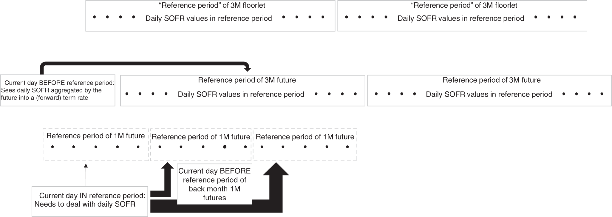
FIGURE 10.1 The aggregation of daily SOFR via the future before the reference period starts and via floorlets
Source: Authors
- In case exposure to the secured–unsecured basis (see Chapter 4) is acceptable, one might think of options on ED futures. However, this does not lead to a decent solution: The option on the ED future covering the same period ends trading on the next business day (Monday), and the option on the following ED contract in the strip has a different period as underlying.
- This only leaves options on 1M SOFR futures as replacement for the expired option on 3M SOFR futures. When the option on the 3M SOFR future stops trading, the “current” day (Figure 10.1) lies somewhere in the middle of the reference period of the front-month 1M SOFR contract. Hence, to cover the whole period of the floorlet, one would need to use a combination of an exotic Asian option (front month) and of standard options (back months) on 1M SOFR contracts. As one progresses through the period underlying the floorlet, these standard options also will become exotic as soon as their contracts enter their reference months.
Since there are only options on 1M SOFR futures left as reasonable hedging instruments without a basis,3 the practical hedger will now be confronted with the problem of a missing pricing formula for Asian options using arithmetic averaging (and of the American type, to make it even more complicated). While the early end of trading in options on 3M SOFR futures spares him encountering this difficulty with 3M future options, in case he wants to maintain his hedge, he will face it when looking at 1M future options as a replacement.
In the absence of a pricing formula (or an approximation with the same first two moments, as explained by Vyncke, Goovaerts, and Dhaene (2003)), the Greeks cannot be calculated. Thus, a possible reaction to this problem could be to only hedge the payoff of the floorlet with a series of options on 1M SOFR futures, but keep exposure to changes in implied volatility, for instance, after the option on the 3M SOFR contract has expired. The next section describes how this could be done without using any (nonexisting) option pricing formula. This approach is risky, if the hedge needs to be unwound before the payment date of the floorlet.
In order to obtain some hedge against changes to the implied volatility (and thereby reduce the risk in case of unwinding the hedge early), one could use options on back-month 1M SOFR futures (in Figure 10.1, this would be the second and third boxes in the row representing 1M SOFR contracts). Since these are still standard options, one can calculate the Greeks both for the floorlet and the future options and thereby the hedge ratios needed for immunity against changes to implied volatility, for example. Of course, this “hedge” is far from perfect (already due to the date mismatches), requires constant adjustments – and ends when the last 1M SOFR future in the floorlet period (third box in Figure 10.1) enters its reference month and the Greeks cannot be calculated anymore. That method therefore only shortens the period of unhedged exposure from about 3M to about 1M.
Without a pricing model (step 2 from Chapter 5), it is impossible to assess, compare, and address the mismatches involved in different hedging approaches theoretically. And without a liquid market, it is impossible to test them empirically (step 3). Unlike in Chapter 9, we can thus neither offer a simple method to deal with mismatches nor look at their magnitudes (as in Figure 9.4). One needs to accept that the current situation does not allow easy or perfect hedges of SOFR-based caps and floors with options on SOFR futures.
Though we can provide neither mathematical proof nor empirical evidence, a practicable hedging strategy for a SOFR-based floor could consist of the following elements:
- Use options on 3M SOFR futures as long as they trade.
- Once they expire, switch to the basic hedging strategy of the payoff of the next floorlet described below.
- If there is a possibility that the hedge needs to be unwound early, reduce the period of unhedged Greeks by using options on back-month 1M SOFR futures as long as this is possible. In this case, it may be advisable to switch from 3M to 1M futures options some days before the former expire in order to avoid the instability problem.
BASIC REPLICATION STRATEGIES OF CAPS AND FLOORS WITH 1M FUTURE OPTIONS
The shift to SOFR has incorporated into the life of options a sudden jump into unknown territory, deprived of the support of a pricing model, leaving only basic approaches available. An analogy could be a researcher being thrown by a plane crash into an untouched (exotic option) world, who needs to rely on elementary techniques for survival until help (from a pricing model) arrives. We will briefly review some of these basic replication and hedging methods, which do not require a pricing formula.
The most straightforward method to ensure earning a minimum interest rate is to simply buy a floor at that minimum rate and to hold it until expiry. As this does not involve any (delta) hedging, no pricing model (or an approximation for calculating the Greeks) is needed. The same can be obtained by buying a series of calls on consecutive 1M SOFR futures at a strike of 100 minus the minimum interest rate desired. Given the early end to trading of options on 3M SOFR futures, options on 1M futures are preferable. But given the limited number of expiration dates listed, this only covers the next three to four months and does not provide strikes far out-of-the-money. (See Chapter 5.) For example, a floor on the average SOFR from January to March 2022 at 0.2% can be achieved by buying calls with a strike of 99.80 on each of the three 1M SOFR futures from January to March 2022. Similarly, a cap at 0.2% can be obtained by buying puts with a strike at 99.80.
Hence, one can consider a series of options on consecutive SOFR futures as replications of caps and floors and use them as a basic hedge. For instance, a dealer short the floor from the example above could buy the series of calls on 1M SOFR futures as an approximate hedge. This is a crude method, of course, which does not take into consideration any different impact of changes in the implied volatility on the (standard) floor and the set of (exotic) futures options. If the hedge needs to be unwound before expiry, this can result in significant losses.
Moreover, while the method of buying a series of calls on consecutive 1M SOFR futures at a strike of 100 minus the minimum interest rate desired will achieve the goal of guaranteeing that minimum interest rate (just like buying a floor), it is quite likely that it costs more than necessary. Imagine that an investor wants to earn at least 0.1% interest during the month of February 2022 and therefore purchases a call with strike 99.90 on the 1M Feb 2022 SOFR future, and that during the first two weeks of February, the daily SOFR values have been 0.2%. By looking at the settlement formula using an arithmetic average, the investor figures out that he is going to achieve his goal of earning at least 0.1% in case the average SOFR during the remaining two weeks exceeds 0.0%. Hence, he can sell his call with strike 99.90 and buy a cheaper call with strike 100.00, thereby reducing the cost of his hedge while still ensuring to meet his goal.
Formalizing this idea, as more and more SOFR values become known, it is possible to adjust the strike accordingly by using the formula
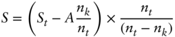
where
- S is 100 minus the adjusted strike for the day when nk days of the reference period are known.
- St is 100 minus the strike over the whole reference period.
- A is the arithmetic average over the known SOFR values.
- nk is the number of known days of the reference period.
- nt is the total number of days of the reference period.
In the example above, S is 0, St is 0.1%, and A is 0.2%. Also note that for St = A, it follows that S = St.
By adjusting the strike of the call via this formula, theoretically every day, it is possible to ensure receiving a minimum interest rate without paying too much.4 For longer periods, the formula can be expanded to cover a series of options on 1M SOFR futures. Using the case from above, where a floor on the average SOFR from January to March 2022 at 0.2% is desired and assuming that the average of SOFR during January and February was 0.3%, a call with a strike at (about5) 100.00 on the March 2022 contract would be sufficient to achieve this goal.
Figure 10.2 shows an example of this cost-minimizing strategy for the month of June 2018, during which the daily SOFR values first dropped from 1.81% to 1.69%, before increasing to more than 2%. Applying the formula above for daily strike adjustments, to achieve a floor at 1.8%, the strike of the call needs to be adjusted downward (resulting in a loss) to a level of 98.15 on June 14, before the increase in SOFR values allows an adjustment upward (resulting in a profit), ending at 98.55. In contrast, to achieve a floor at 1.9%, the strike of the call needs to be constantly adjusted downward, since the daily SOFR values were quite a bit below 1.9% at the beginning of the month and even their increase toward the end of the month could not bring the average toward 1.9%. As a consequence, this strategy required a significant strike adjustment in the later period, ending at a strike of 97.05 – while the loss was mitigated by the low time value.
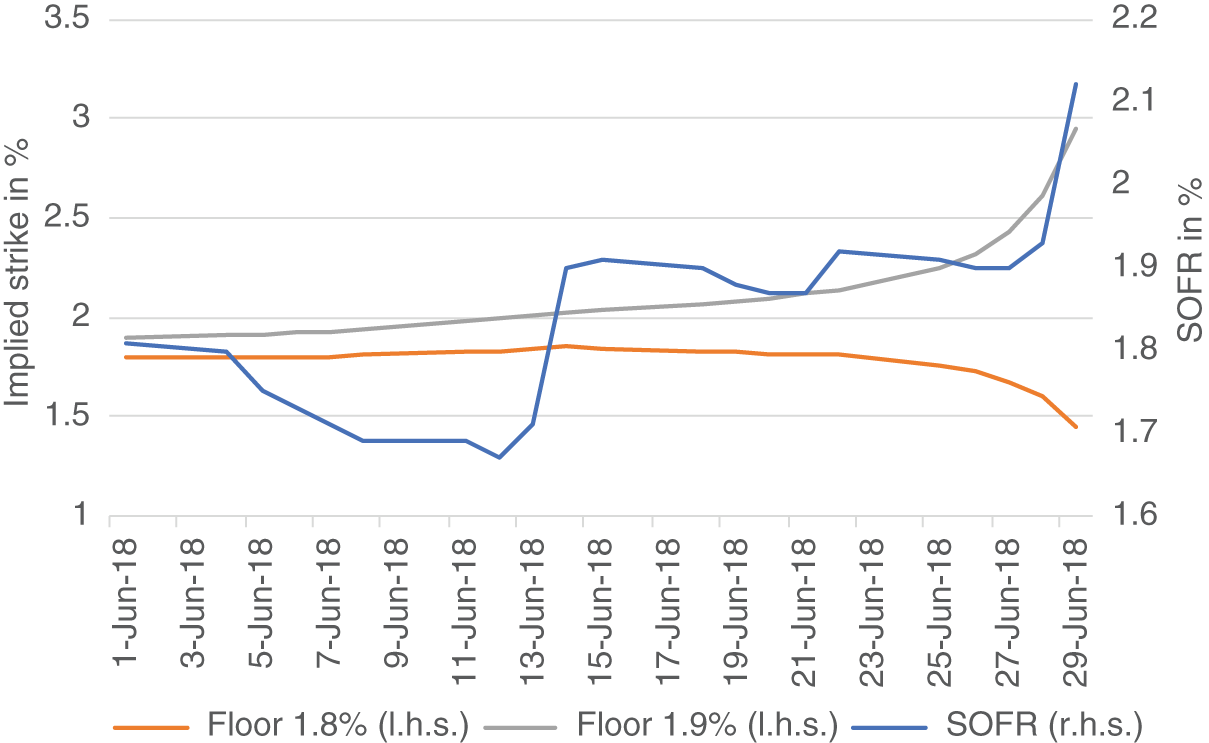
FIGURE 10.2 Implied strikes for obtaining a 1.8% and a 1.9% floor during June 2018
Source: Authors, from CME data
It is tempting to compare this strike adjustment strategy with similar observations from options trading:
- Like the Black-Scholes approach transfers the P&L from a payment at expiry to P&L from delta hedging before expiry, so does this strategy to P&L from strike adjustments before expiry.
- Like some Greeks (such as gamma for ATM options) converge toward infinity immediately before expiry, so does the adjusted strike level.
- Moves in the underlying cause the P&L of delta hedging as well as of the strike adjustments. But in the latter case only, the skew matters, too. In fact, close to expiry, exposure to the skew can become substantial due to the large adjustments required.
Together with the fact that all variables used in the formula above will also occur in any option pricing formula, these similarities make it likely that the basic strike adjustment strategy will collapse into model-based option trading, once it is available. While the precise form of this integration will depend on the precise form of the pricing formula, two possibilities seem conceivable:
- A collapse into delta hedging along the approach of Black-Scholes. For this to become possible, only the Greeks need to be known, for which approximations along the lines of Vyncke, Goovaerts, and Dhaene (2003) are sufficient.
- A collapse into Asian option pricing with floating strikes. Once such a model will be available, this appears to be a natural integration for the elementary strike adjustment strategy.
DEALING WITH DAILY FLOORS
Another problem arises from the recommendation of the Alternative Reference Rates Committee (ARRC) to apply the floors of some loans to each daily SOFR value rather than the SOFR compounded over the reference period. Due to the early-repayment option of the borrower in business loans, ARRC argues for flooring the daily SOFR values (Federal Reserve Bank of New York 2020a; Federal Reserve Bank of New York 2020b). In this case, the floor has a different underlying than the options on SOFR futures, which refer to the SOFR compounded or simply averaged over the reference quarter. This leads to a further mismatch between the floor and the options on SOFR futures as potential hedging product, resulting in even more risk and/or higher hedging costs. In fact, if a perfect hedge is the goal, options on SOFR futures cannot be used for hedging floors following the ARRC recommendation, even if a pricing formula existed. Figure 10.3 illustrates this additional problem.
Conceptually, a floor based on ARRC's recommendation is a set of standard options, while the options on SOFR futures used for hedging are exotic options. Even after a pricing model for the latter will have become available and hence the difference between standard and exotic options will be assessable, the difference between a collection of daily options and an option on the arithmetic average or compounding of these daily values will continue to exist. At this future stage, one could try to tackle this difference by a theory for the spread between an (exotic) option on a portfolio and (standard) options on each of the components of the portfolio, consisting in this case of the daily SOFR values and hence of highly correlated variables.
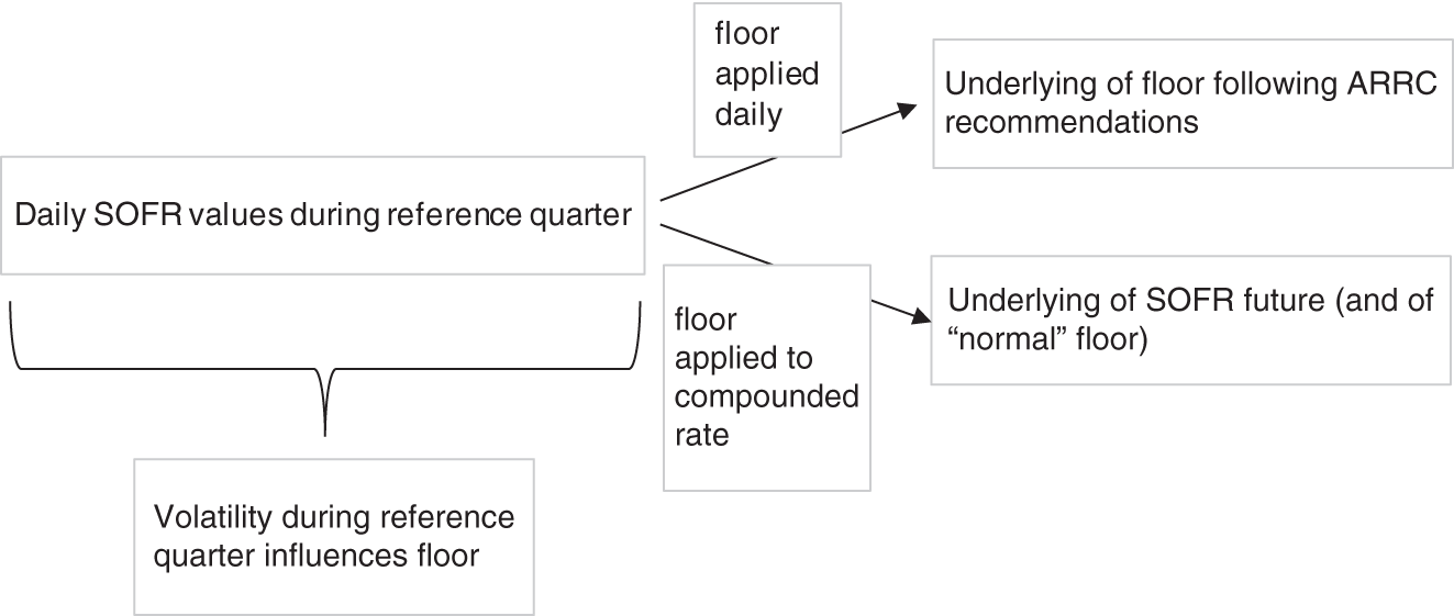
FIGURE 10.3 Underlying of SOFR-based floors and options on 3M SOFR futures
Source: Authors
At the current stage, however, we can only provide a first impression about the magnitude of the mismatch between a floor on daily SOFR values and a floor on SOFR compounded over the whole reference quarter by further expanding the simulation sheet (used for step 1 toward a pricing model in Chapter 5). As before, this should be considered as an initial attempt only: Since ARRC's recommendation has introduced a completely new feature, our goal is to provide some basic intuition about the potential severity and driving factors of the mismatch. In order to avoid the problem of the missing pricing formula for options on SOFR futures, we look at the difference between a (standard European) floor over the whole 3M period versus daily (also standard European) floors.
The simulation is encoded in the Excel spreadsheet “Floor simulation” accompanying this chapter, which is a slight modification and expansion of the sheet “Call simulation” from Chapter 5. Again, we assume that on Jan 1, 2022, one wants to price a floor on SOFR during the reference quarter of the Mar 2022 SR3 contract (Mar 16 to Jun 15). During the reference quarter, there is one scheduled FOMC meeting, on May 4, 2022; and – unlike in Chapters 2 and 5 – one can add an unscheduled meeting on Jun 1, 2022, to the simulations. By contrast (also unlike in Chapter 2), we assume that there is zero probability for a change in Fed policy outside of these two meetings, including on the two FOMC meetings before the start of the reference quarter. Of course, one can also run the simulation without this rather unrealistic assumption, but the added complexity of further multiplying the possible parameter combinations is not needed for our current goal, since the difference between the two types of floors depends mainly on the Fed policy changes occurring during and not before the reference period.
As in Chapters 2 and 5, column E defines the parameters for the Vasicek process and the probability distribution for the jump at the FOMC meeting(s). For each of the simulated paths, the value of a floor (with the level of the floor being set in cell H1, just as the strike of the call has been set in Chapter 5) is calculated both for the daily floor as recommended by ARRC for loans with a prepayment option and for the floor on the whole compounded 3M period. The average floor values over all simulations and the premium for daily floor application (in percentage terms) are displayed in column H. For example, if the value for the daily floor is 11 bp and for the floor over the whole period 10 bp, a premium of 10% is shown in cell H5.
Table 10.1 summarizes the results of this simulation for a number of different input parameters. The key observation is that the premium can be significant if a jump process is used,6 but is limited when a diffusion process is applied. For a pure jump process with the scheduled Fed meeting on May 4 only, the premium for the daily floor over the floor for the whole period is 44% if one assumes an equal probability distribution for a 25 bp hike, no action, and a 25 bp cut. If a second Fed meeting takes place on June 1 with the same probability distribution, the premium increases to 72%. This can be explained intuitively by imagining the paths of SOFR entering the reference quarter at 5 bp (for a pure jump process, this is the case for all paths) and dropping to –20 bp at the first meeting. As the compounded 3M rate is still above 0%, the floor applied to the whole period expires out-of-the-money, whereas every day with an SOFR at –20 bp contributes to the payoff of the floor applied daily. Taking this to an extreme, if the Fed was certain to cut by 25 bp on May 4 and hike by 25 bp on June 1, the premium for the daily floor would increase to 129%.
For a pure diffusion (with drift) process, on the other hand, the premium is much less pronounced. It seems to slightly increase with the speed of mean reversion, and it clearly decreases when the level of the floor increases. Combining both processes to a jump-diffusion (with drift) process, the premia lie between the high levels of the jump process and the low levels of the diffusion process, as one would expect. For the parameters shown in Table 10.1, the premia of the jump-diffusion process are much closer to the ones of the pure diffusion (with drift) process. However, this could change when the overall contribution to the floor value from the jumps becomes relatively larger (e.g., due to more FOMC meetings and/or larger jumps).
Overall, one could be tempted to conclude preliminarily that in case of a diffusion process, the premium introduced by the ARRC recommendation to apply the floor daily is limited; one might deal with it by first calculating the usual hedge ratio for normal floors (covering the whole period) and then “overhedge” by increasing the hedge ratio by, say, 10%. In case of a jump process, however, the premium is larger and depends on the precise dates of the FOMC meetings as well as the probability distributions of Fed action. This cannot be handled by a simple adjustment anymore. It is interesting to see the relationship of the specific problem of the daily floor to the general problem of process selection described in Chapters 2 and 5:
TABLE 10.1 Simulated premium of daily versus compound caps in %
Source: Authors
| MAIN CASE 1: ONLY JUMP(S), start value 0.05%, floor at 0% | ||||||||
|---|---|---|---|---|---|---|---|---|
| Subcase 1a: Only FOMC meeting on May 4 | ||||||||
| Probability of +25 bp Jump | Probability of 0 bp Jump | Probability of –25 bp Jump | Premium | |||||
| 50% | 0% | 50% | 44% | |||||
| 50% | 50% | 0% | 0% | |||||
| 33% | 34% | 33% | 44% | |||||
| Subcase 1b: Also unscheduled FOMC meeting on June 1 | ||||||||
| May meeting | June meeting | |||||||
| Probability of +25 bp Jump | Probability of 0 bp Jump | Probability of –25 bp Jump | Probability of +25 bp Jump | Probability of 0 bp Jump | Probability of –25 bp Jump | |||
| 50% | 0% | 50% | 50% | 0% | 50% | 47% | ||
| 33% | 34% | 33% | 33% | 34% | 33% | 72% | ||
| 0% | 0% | 100% | 100% | 0% | 0% | 129% | ||
| MAIN CASE 2: ONLY DIFFUSION AND DRIFT | ||||||||
| Start value | Standard Deviation (ann) | Mean | Speed of Mean Reversion | Floor | Premium | |||
| 0.05% | 2% | 1.50% | 0 | 0% | 7% | |||
| 0.05% | 5% | 1.50% | 0 | 0% | 7% | |||
| 0.05% | 2% | 1.50% | 0.002 | 0% | 10% | |||
| 0.05% | 5% | 1.50% | 0.002 | 0% | 10% | |||
| 0.05% | 2% | 1.50% | 0.002 | 1% | 3% | |||
| 0.05% | 5% | 1.50% | 0.002 | 1% | 5% | |||
| MAIN CASE 3: JUMP-DIFFUSION (AND DRIFT) | (only FOMC meeting on May 4) | |||||||
| Start value | Standard Deviation (ann) | Mean | Speed of Mean Reversion | Floor | Probability of +25 bp Jump | Probability of 0 bp Jump | Probability of –25 bp Jump | |
| 0.05% | 2% | 1.50% | 0 | 0% | 50% | 0% | 50% | 8% |
| 0.05% | 2% | 1.50% | 0 | 0% | 33% | 34% | 33% | 7% |
| 0.05% | 2% | 1.50% | 0.002 | 0% | 50% | 0% | 50% | 14% |
| 0.05% | 2% | 1.50% | 0.002 | 0% | 33% | 34% | 33% | 12% |
| 0.05% | 5% | 1.50% | 0.002 | 0% | 50% | 0% | 50% | 11% |
| 0.05% | 2% | 1.50% | 0.002 | 1% | 50% | 0% | 50% | 3% |
| 0.05% | 2% | 1.50% | 0.002 | 1% | 33% | 34% | 33% | 4% |
- If one decides to use a diffusion process, the daily floor can probably be incorporated via a rather small premium.
- If one decides to use a jump process, the daily floor needs to be modeled directly.
NOTES
- 1 During the editing process of this book in the first half of 2022, liquidity in options on SOFR futures has started to increase.
- 2 On the Friday before the 3rd Wednesday of the contract month. See Figure 5.2 for more details.
- 3 Apart from OTC products, which are costly and only pass on the pricing problem without solving it.
- 4 From the perspective of setting the strike level of the option on the 1M SOFR future. Of course, it is possible that there are cheaper alternatives from using other options.
- 5 Ignoring the different number of days in these three months.
- 6 In the Excel spreadsheet, this can be obtained by using very small numbers in cell E2, such as 0.000001. Using 0 as parameter will not work due to the set-up of the simulation.