
CHAPTER 9
Hedging Swaps and Bonds with SOFR Futures: The Convergence of Futures, Swaps, and Treasury Pricing Following the Transition to SOFR
In order to present the big – and beautiful – picture, let us ignore some ugly details like daycount conventions for a moment. One major consequence of the transition from LIBOR to SOFR is the fact that SOFR futures, SOFR swaps, and government bonds become conceptually very similar:
- 3M SOFR futures compound consecutive 3M forward periods of SOFR into a forward rate and hence the SOFR futures strip into a term rate.
- Swaps with SOFR as floating-leg exchange SOFR versus a fixed-term rate.
- Treasuries can be considered as exchanging their funding rate at (a level close to) SOFR for their coupon payments.
Hence, all three instruments – futures, swaps, and Treasuries – can be seen as (slightly different) ways to compound the same reference rate, daily SOFR values (or, in case of Treasuries, the repo rate, which is typically close to SOFR), into a term rate. Allowing for some imperfection in order to express the conceptual similarity, one could say that futures strips, SOFR-based swaps, and Treasuries all combine the same underlying SOFR into term rates. Abstracting from the technical differences, one might therefore consider all three instruments to be essentially the same – i.e., market prices for a certain future segment of daily SOFR.
Before adding the technical differences, let us contemplate the general consequences of this observation. With futures strips, swaps and Treasuries having become essentially the same, one can replicate and hedge one with another. Furthermore, one can establish arbitrage relationships between the three, which will provide additional sources of profit for relative value (RV) traders and enhanced liquidity in the interconnected instruments for every market participant.
These practical benefits, together with the conceptual beauty of three key markets converging toward essentially the same instrument, can be considered as a major advantage of the transition from LIBOR to SOFR. Expressing some aspects of this advantage more specifically:
- Before the financial crisis, LIBOR-based swaps used the same curve both for determining the cash flows and for discounting. The switch to discounting with another curve (Fed Funds and later SOFR) following the financial crisis resulted in the need to use dual curves when evaluating LIBOR-based instruments. Transitioning everything to SOFR reinstates the clean and easy situation of the old days: SOFR-based swaps usually1 use the same curve – i.e., SOFR, both for determining the cash flows and for discounting. One consequence is that the present value of the floating side at inception is equal to 100.
- And the daily SOFR values are usually compounded for calculating cash flows and discount factors in the same manner as the settlement price of 3M future contracts. (See formula in Chapter 2.) Hence, the futures strip as defined in Chapter 2 applies the same calculation as SOFR-based swaps. In the following, we will use the futures strip rate as the discounting curve. It is easy to adjust this for other agreements, such as a two-day payment delay.
- Moreover, while the first floating payment of a LIBOR-based swap was usually known at the start of the swap (e.g., the current 3M LIBOR), the first floating payment of a SOFR-based swap refers to the reference period starting after entering the swap and is hence unknown. This rectifies the unintuitive feature that only nine months of a 12M LIBOR-based swap are unknown and hence affected by changes to the yield curve. For 12M SOFR-based swaps, the whole 12 months are unknown at the start of the swap. And this also aligns SOFR-based swaps with SOFR futures. The increasing portion of known values (see Figure 2.4) will result in an (almost) equal decrease of sensitivity to interest rate changes of both the swap and the future strip – a fact that stabilizes the hedge ratio of a futures strip.
- Regarding government bonds, we have explained in Chapter 4 that the migration to SOFR-based asset swaps eliminates the basis between unsecured and secured rates inherent in LIBOR-based asset swaps. Going one step further, with Treasuries being conceptually the same as a basis swap between their funding rate (individual repo) and their coupon rate, one immediately sees the link to a SOFR-swap between repo rates and the fixed rate. Assuming a Treasury always could be financed at SOFR (i.e., it never becomes special), and ignoring payment frequency and daycount differences as well as differences in regulatory treatment, the transition to SOFR allows us to consider swaps and bonds to be conceptually the same – an exchange of an overnight secured funding rate (SOFR) with a fixed rate. And the swap and bond markets are two different places to get a price for the same collections of future SOFR values (e.g., over the next two years). Another way to express this link is to say that, under these assumptions, the fair value of a Treasury asset swap spread is zero.
Unfortunately, one needs to add back the abstractions and simplifications, thereby introducing some complexities into this beautiful and clean picture:
- While the repo rate of individual Treasury bonds is usually close to SOFR, differences are possible due to specialness effects. As SOFR excludes most of the specialness and can be considered as a general collateral (GC) rate, the financing rate of a specific Treasury could be special, for example, because it is a benchmark or cheapest-to-deliver (CTD) into a bond futures contract. In this case, the compounded expected daily financing rates of a Treasury bond, i.e., its yield, should be lower than the compounded expected SOFR (i.e., the futures strip rate, ceteris paribus, including daycount and payment frequency). However, in the range of the yield curve covered by SOFR futures, specialness is usually absent due to the absence of its main causes, benchmarks, and CTDs. It is even possible that on days with a particularly large share of special repo rates – e.g., due to high transaction volume in a 10Y benchmark – not all of this effect is excluded during the SOFR calculation and that thus SOFR would be below the repo rate of a specific Treasury. In summary, for shorter Treasuries, it should usually be fine to assume SOFR ≈ Repo and hence equality of the foundation in Figure 9.1.
- Regarding the integration of the daily rates (SOFR and individual repo) into term rates, a variety of different technical features complicates the task of comparing the three markets. Among these are different payment frequencies (e.g., 3M for futures and 6M for treasuries) and daycount conventions (usually actual/360 for money market and actual/actual for Treasuries). Moreover, as an OTC product, the swap counterparties can agree to all sorts of discounting curves and payment times. For example, SOFR-OIS cleared by the CME have a two-day payment delay. On top of all this comes the issue of date mismatches, highlighted in Chapter 7.
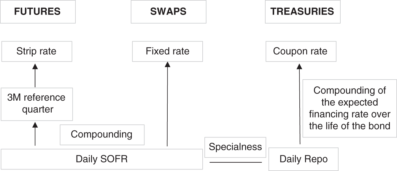
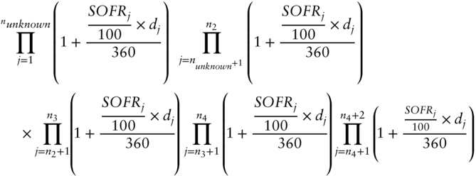
FIGURE 9.1 Integration of SOFR into a term rate in the future, swap, and Treasury markets
Source: Authors
- And also the impacts from the regulatory side need to be considered. As mentioned in Chapter 4, it can be beneficial for a bank to hold Treasuries rather than engaging in swaps from the perspective of capital costs. The extent of this benefit – and hence the premium the bank is willing to pay for Treasuries – depends on the proximity of balance sheet constraints, which is hard to observe and to quantify. (See Chapter 1.)
Despite these caveats, however, the close link between the three markets introduced by the transition to SOFR can still be used as the basis for replicating and hedging, in particular with SOFR future strips. Figure 9.1 illustrates these links and the remaining part of this chapter will further investigate and exploit them. First, we will provide empirical evidence for the conceptual similarity of SOFR futures and government bond markets. Then, we will apply the return to the good old days of a single curve to replicate the hedging of LIBOR-based swaps with ED futures strips for hedging SOFR-based swaps with SOFR futures strips. Finally, after exploiting the proximity between swaps and Treasuries to transfer this method to hedging Treasuries with SOFR future strips, we will follow one specific Treasury hedge over time and discuss its management and actual performance.
In contrast to the convergence of the markets for swaps and government bonds, the transition from the unsecured funding rate LIBOR to the secured funding rate SOFR has caused a divergence of the markets for (SOFR-based) swaps and corporate bonds. Actually, hedging a corporate bond with a SOFR-based swap now involves the same unsecured versus secured basis (credit risk) that was involved in hedging government bonds with LIBOR-based swaps (Burghardt, Belton, Lane et al. 1991, p. 110). Hence, we do not recommend hedging corporate bonds with SOFR-based swaps or futures – unless to intentionally express a view on the unsecured versus secured basis – but rather to use ED or FF futures as mentioned in Chapter 4.
TREASURIES VERSUS SOFR FUTURES STRIPS
Building on Chapter 4, we have just argued via Figure 9.1 that, due to the proximity of the financing rate (i.e., the repo rate of the individual Treasury) to SOFR, the asset swap spreads of Treasuries should usually be close to zero (when the swap uses SOFR as floating leg), or equivalently, that the Treasury yield should usually be close to the SOFR futures strip. Intuitively, both the Treasury yield and the SOFR futures strip can be thought of as slightly different ways to compound the expectations about very similar daily financing rates into a term rate.
In order to provide some empirical evidence for this argument, we have calculated the 1Y and 2Y SOFR futures strip rates at the beginnings of the last four reference quarters (Dec 2020, Mar, Jun, and Sep 2021), using the same simplifications2 as outlined in Chapter 5 and the formula for the strip rate calculation from Chapter 2. This strip rate compounds the daily SOFR values into a term rate using money market daycount conventions; in order to compare it with semiannual bond yields, the following formula has been applied:
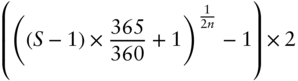
where
- S is the strip yield as calculated in Chapter 2, i.e., by compounding all daily SOFR values.
- n is the number of years (1 or 2).
Figure 9.2 shows the difference between the constant maturity Treasury (CMT) yield as published by the Federal Reserve Economic Data (FRED) database and the SOFR futures strip rates as calculated in the manner above. Overall, the differences are small – in line with the goal to validate the argument above. This proximity is also the basis to replicate and hedge Treasuries with SOFR futures strips.
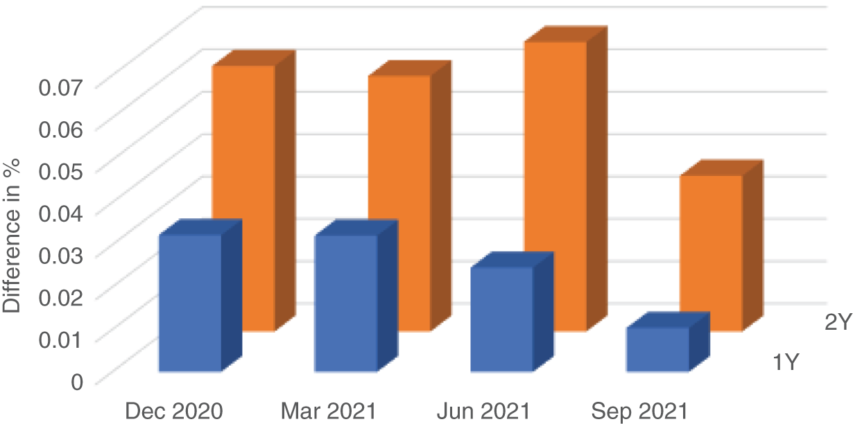
FIGURE 9.2 CMT minus future strip yields
Source: Authors, from CME and FRED data
The positive differences visible in Figure 9.2 mean that the CMT yields have been slightly above those of the futures strips. This could be explained by the following factors:
- As usual, specialness has been largely absent from 1Y and 2Y Treasuries. Hence, specialness of 10Y benchmarks, for example, might have caused SOFR to quote below the individual repo rates of short Treasuries (see above).
- Due to the low interest rate environment and easy access to funding, leverage restrictions have played no major role for the pricing during the last year. In terms of Chapter 1, the regulatory cost affecting RV relationships has been close to zero and hence the preference for Treasuries for regulatory reasons has been negligible.
- Effects from the simplification of the reference quarters and from the calculation method of the CMT could also be involved.
When trying to extend this analysis further back, we face the issue of less liquidity in the SOFR futures, especially in the later part of the 2Y strip. Abstracting from these problems (and from those of the simplifications), the general picture provided by Figure 9.2 still holds: slightly positive spreads of a few basis points and more so for 2Y maturities than for 1Y maturities. And we also observe an instance of negative spreads during the period of spikes in SOFR. In March 2020, during the sharp drop in interest rates, there was a period of exceptionally cheap Treasuries relative to the futures strip. We will choose this period intentionally for the analysis of the performance of a Treasury hedge with futures; the discrepancy will show up as a gap between the lines of Figure 9.4.
HEDGING SOFR SWAPS WITH SOFR FUTURES
This section starts by exploiting the move back from dual curves to a single curve to replicate the hedging method of swaps with LIBOR as the floating leg and as discount curve with ED contracts in the ideal case of an IMM swap. We will then consider the adjustments required in less ideal and more realistic circumstances as well as for the recent evolution of the typical conventions for SOFR swaps, ending with an example of hedging of what might currently be the most common SOFR swap.
Due to the novelty of SOFR swaps and their conventions, most of the material in this chapter – and in some other chapters as well – is original and has not been subjected to years of practical application in the market. It is therefore likely that additional aspects not covered here will surface over time when using our approach. The methods and formulae should therefore be considered only as a conceptual starting point, which the reader will probably need to adjust when applying to actual hedges, for example, to reflect further evolutions of the conventions. This comes on top of the necessary adjustment for his specific hedging goals, as mentioned in Chapter 2 and in the introduction to section 2.
As a starting point, let us assume that the SOFR swap replicates the typical conventions of an IMM LIBOR swap:
- The fixed side pays quarterly coupons using bond conventions (30/360).
- The floating side also pays quarterly rates using money market conventions (Actual/360), with the 3M LIBOR being replaced by the compounded SOFR during the 3M reset period (using the ISDA formula from Chapter 2).
- The same compounded SOFR is used as discount factor.
- The reset periods of the swap coincide with the reference quarters of the SOFR futures, as is the case with IMM swaps.
- The payment dates of the swap match those of the futures, i.e., there are no payment delays.
The perfect match of the conventions between futures and swap markets achieves the goal of demonstrating the ideal case in the sense of the conceptual discussion above; the replication of the conventions of LIBOR swaps achieves the goal of demonstrating the link to the hedging method with ED futures. We are aware that both assumptions are rather unrealistic given the current typical conventions for SOFR swaps (with a payment delay and money market conventions also on the fixed side, among others) and will address the necessary adjustments after presenting this artificially ideal case.
In a nutshell, the hedge of such a swap using SOFR as floating leg with SOFR futures can be done in the same manner as Burghardt, Belton, Lane et al. (1991, p. 98) describe hedging a swap using LIBOR as floating leg with ED contracts: Determine the sensitivity of the swap to each forward rate and hedge it with the corresponding ED future, thereby obtaining immunity against movements in all parts of the forward curve. This is possible since both the cash flows and the discounting curve are the same (SOFR) again.
In more detail, assume a 1Y swap starting on Jun 16, 2021, and exchanging on the contract dates (Sep 15 and Dec 15, 2021, and Mar 16 and Jun 16, 2022) of the 3M SOFR futures a fixed rate of 1% (quarterly 0.25%) versus the floating rate as defined by the compounded SOFR values during the previous swap period, which is assumed here to match the reference quarter of the contract. IMM swaps, which have been constructed according to the specifications of their hedging instruments, fulfill this assumption, which makes hedging with futures easy. Also assume that the payments in the swap occur at the same time as the future settlement, i.e., without an offset like for CME-cleared SOFR OIS. Under these ideal assumptions, the floating payments in the SOFR-based swap are exactly the settlement payments of the SOFR futures strip.
The present value of this swap3 (for receive fixed, pay floating) is given by:
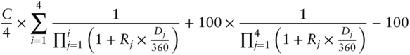
where
- C is the annual fixed coupon, in this example assumed to be 1%.
- Rj is the (forward) rate for the jth period of the swap, in this example matching the reference quarter of the jth future in the strip, thus Rj = 100 – price of the jth future.
- Dj is the number of calendar days in the jth period.
It is instructive to compare this formula with the one from Burghardt, Belton, Lane et al. (1991, p. 98):4 Unlike for LIBOR swaps, the first floating payment is unknown for SOFR swaps, resulting in the present value depending on the first rate as well. Also note that the term –100 at the end of the expression is the present value of the floating side in this ideal circumstance, where both the floating payments and the discount curve are calculated by exactly the same compounding formula.
Based on this formula, one can now calculate the sensitivity of the present value of the swap to each rate period of the futures strip. This can be done analytically by differentiating the formula by Rj or numerically by recalculating the present value after bumping a specific Rj by 1 bp and taking the difference. The latter method is encoded in the sheet “Swap hedge with strip” accompanying this chapter: The effect of a 1 basis point (bp) increase in the Rj from column D is calculated in cell D12 and pasted into column I. One can then immunize against the effects of changes in each forward rate (Rj) by selling the corresponding futures contract. The hedge ratio is obtained by dividing the change of present value (for a given notional, in this example USD 100m in cell C14) (column J) by the basis point value (BPV) of the futures contract, USD 25. This results in a hedge of short 102 Jun 2021, short 102 Sep 2021, short 101 Dec 2021, and short 101 Mar 2022 SR3 contracts (column K). The money market conventions explain the fact that more than 100 futures are needed for each period. The decreasing discount factor (column G) explains the fact that the number of futures decreases with an increasing forward horizon.
This result suggests that a good approximation for the hedge could be obtained by an easier method: Calculate the change of present value of the swap in USD for a parallel curve shift (rather than for each individual consecutive forward rate), divide the result by 25 to get the total number of futures, and divide it equally over the futures contracts in the strip. The condition for this approximation to work well is that the discount factors are all close to 1, which is the case in the example above. However, for higher rates and/or longer tenors of the swap, the discount factors will be less close to 1 (and to each other) and thus the simpler method will produce a less accurate approximation for the hedge against moves in any consecutive forward rate.
Moving from the ideal to the real world, we now consider the necessary adjustments for more typical conventions and less perfect matches between the dates. Regarding the conventions:
- Using money market conventions (Actual/360) for both the fixed and floating leg seems5 to be the current norm for SOFR swaps. This results in the position of the discrepancy between bond and money market conventions moving from within swaps (between fixed and floating leg) to the external relationship between bonds and swaps. As long as bonds do not apply money market daycount conventions, the discrepancy will not disappear, for example, from asset swaps, but rather than being located between the fixed and floating leg of the swap, it now occurs between the bond and the fixed leg of the swap.
This change can easily be incorporated into the present value formula above and hence into the hedge based on it by multiplying C with 365/360.
- SOFR OIS cleared by the CME use a two-day payment delay for the floating side (and of zero or two days for the fixed side) according to CME (Q4 2018, p. 7) (see Chapter 3 for more background). This can also easily be incorporated into the formula by extending the time frame for calculating the discount factor accordingly. If only the floating side uses the payment delay, two different discount factors need to be applied. And this introduces a mismatch between the floating payment and the discount factor again, resulting in the present value of the floating side becoming different from 100 even at inception. While the discrepancy is usually not as high as in cases of using dual curves with a basis between them, the term for the present value of the floating side becomes more complicated than the simple –100. Moreover, moves in SOFR after the start date of the swap result in a deviation of the present value of the floating side from 100 even in the ideal case of a perfect match at inception.
- Most SOFR swaps appear to apply annual payments for both the fixed and the floating leg. Accordingly, rather than discounting each individual quarterly payment as above, the netted payment is discounted annually. For the hedging method, this means that the “natural” decomposition of the discount factors into the segments of the SOFR futures strip needs to be “artificially” created. But with this little trick, shown in the formula breaking down S below, the same approach can be used.
And regarding date mismatches:
- If the start date of the swap does not correspond to the start date of a reference quarter (unlike for the ideal IMM swap considered above), the first SOFR futures contract used for hedging is already in its reference quarter. This can be handled by applying the techniques presented in Chapter 2. In fact, the artificial decomposition of the discount factor mentioned above and expressed mathematically below will then have Runknown as first segment.
The further the start date of the swap falls behind the start date of the reference quarter, the more SOFR values are already known. This results in a lower sensitivity of the SOFR futures contract to changes in the SOFR level, since they only affect the remaining reference quarter. But the same is true for the sensitivity of the swap, which also depends only on the unknown part of SOFR values. In an ideal case, the decreases of sensitivity of the swap and its hedging instruments are equal, allowing us to keep the hedge ratio stable even as the front-month contract progresses through its reference quarter (only adjusting the hedge ratio for the increase of the discount factor over time). Depending on the conventions (and the level of known SOFR values) it is theoretically possible that the passing of time affects the sensitivity of the swap and the futures hedge unevenly. But the results of the examples shown below suggest that simply keeping the hedge ratio of the front month stable until settlement seems to work usually well in practice.
We lack experience about the practicability of maintaining the hedge during the last days of the reference quarter into settlement, though; after applying these concepts in the actual market, it may well turn out that rolling the hedge with the front month into the first deferred contract month, for example, three days before it expires, works better.
- If the end date of the swap does not correspond to the end date of a reference quarter, the last SOFR futures contract used for hedging will cover a period going beyond the swap term. If no FOMC meeting falls between the two end dates, it is usually6 acceptable to continue using the futures strip without adjustment. If an FOMC meeting takes place between the two end dates, however, the adjustment techniques described in Chapters 2 and 7 need to be incorporated, for example, by calibrating a jump(-diffusion) process.
Figure 9.3 illustrates the date mismatches at the beginning and at the end of the futures strip covering the swap and the approaches to dealing with them.
Let us now try and combine all these adjustments (with the exception of a mismatch at the end date) into a possible hedge of what is likely to be the most typical SOFR swap with a strip of SOFR futures. Reflecting the currently most common conventions described above, we assume that the 1Y SOFR swap, still starting on Jun 16, 2021, and ending on Jun 16, 2022, exchanges yearly payments of a fixed versus a floating rate, i.e., just once at its end. We further assume that both legs apply money market conventions and a two-day payment delay, i.e., that the payment takes place on Jun 17, 2022. And we calculate the hedge at an arbitrary point in time during the reference quarter of the first contract (Jun 2021), not necessarily at the start date of the swap. As a consequence, we will encounter a different term than –100 for the present value of the floating leg.
For this case, the netted payment is given by the difference of the fixed rate and the compounded SOFR values over the year, both using money market conventions, i.e.:
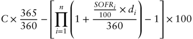
where
- C is again the annual fixed coupon.
- n is the number of business days during the swap period, i.e., i starts on Jun 16, 2021, and ends on Jun 14, 2022.
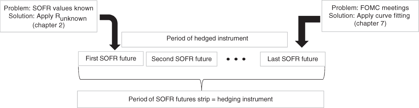
FIGURE 9.3 Date mismatches between the hegded instrument and the SOFR futures strip used for hedging
Source: Authors
- SOFRi is the SOFR for day i (published on the next business day).
- di is the number of calendar days for which SOFRi is used.
The discount factor is determined by the strip rate S from Chapter 2, starting at the present day, in this case assumed to be any day during the reference quarter of the Jun 2021 contract, and extending two business days after the end of the swap, i.e., until the actual payment date. Breaking down S into the segments of the strip, one can write the discount factor in the following form:
where
- j starts at the present day.
- nunknown is the number of business days during the unknown (future) part of the reference quarter of the first contract, as defined in Chapter 2.
- nk is the number of business days between the present day and the last day of the reference quarter of the kth contract.
Dividing the netted payment by the discount factor, i.e., both expressions, returns the present value for the more realistic case. While it looks more complicated than the ideal case described at the beginning, the same idea can be applied to calculate the hedge ratios: Rather than bumping each Rj and observing the impact on the present value, now every SOFRj during each reference quarter needs to be changed. And unlike in the easy case above, this shift now also affects the floating payment, i.e., both the numerator and the denominator of the present value formula.
As starting values for the bump, it seems reasonable to use the known values for SOFR (as in the sheet “Strip” from Chapter 2) and the unknown SOFR values implied by the futures strip. With this adjustment, the same method described above can be applied: Calculate the effect of a 1 bp bump in each of the individual reference quarters on the present value of the swap and obtain the number of futures by dividing by the effect of a 1 bp bump during its reference quarter on the present value of the futures contract. Specifically for the front-month contract, the effect of a 1 bp bump to all SOFR values during the (remaining part of the) reference quarter can be different from the effect of a 1 bp bump to the futures price. Hence, the divisor cannot simply be assumed to be 25 anymore but needs to be calculated as well.
The Excel sheet “Swap hedge with strip 2” encodes this approach toward hedging. We assume the hedge is calculated on the “present day” of June 23, 2021, i.e., one week after the start date of the swap, and incorporate the relevant part from the sheet “Strips” from Chapter 2 to deal with the known part of SOFR values. We use the actual SOFR values for the known part and the SOFR values implied by the futures market of Jun 23, 2021 (column H), for the unknown part (column K).7 For this case, the implied daily SOFR values are extremely close to the future rates.
As a complication, an FOMC announcement is scheduled for June 15, 2022. While this does not affect the futures anymore, it has an effect on the discount curve, which extents two days longer: The SOFR for June 14 is the last value used for calculating the floating rate payment and the prices of the hedging instruments; but the SOFR values for June 15 and 16 are involved in the calculation of the discount factor, and at least the latter is affected by the FOMC decision published on June 15. This is also a good example of the effect that seemingly small convention details like a two-day payment delay can have on the pricing and hedging models. It introduces a new variable (for the Fed policy change on June 15) into the equation, which could be calculated by the jump process fitting method. For this specific case, given the current price of the Jun 2022 contract and the fact that only one or two days are affected, one might decide to not further complicate the sheet by assuming no policy change at the June 15 meeting.
Inputting the same values for C (1%) and the notional (USD 100 m) as before, column K performs the calculations from the formulae above, showing the future rates, the fixed and floating payments, the discount factor, and the present value for the swap for the specific SOFR values (column C). These SOFR values can now be bumped segment-wise via column L. The resulting changes in the present value of the swap and the future rate are displayed in columns M and N, respectively. We note that our expectation, that the sensitivity of the first future contract and the swap decreases to an equal extent as more SOFR values become known, is validated. Using the same method as before, the number of futures required to hedge against those segment-wise changes in the SOFR strip is calculated in column O. For this example, the hedge consists in selling 101 of each of the four contracts, Jun, Sep, and Dec 2021 as well as Mar 2022.
Comparing the results with the easy hedge from the beginning, there is only a marginal difference. Before jumping to the conclusion that the efforts of incorporating all adjustments add little value, the reader should keep in mind that the situation is likely to change when the yield curve is not flat and close to zero anymore.
HEDGING TREASURIES WITH SOFR FUTURES
Exploiting the close link between the three markets described at the beginning and illustrated in Figure 9.1, the approach to swap hedging can be easily adjusted to hedging government bonds with a SOFR futures strip as well. This section starts by describing the modifications before demonstrating a possible hedge for a concrete example. It will then follow the evolution of the hedge over time, discuss the necessary management, and assess its performance.
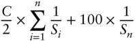
For a Treasury with semiannual coupon payments, the present value is given by
where
- C is again the annual coupon.
- n is the number of coupon payments until maturity.
- Si is the strip rate until the payment date of the ith coupon (as defined in Chapter 2).
As above, the same little trick of decomposing the strip rate into the segments defined by the reference quarters of 3M SOFR futures can be applied. Once the hedging problem is set up in this form, it can again be approached by extracting a curve of daily SOFR values from the current SOFR future prices,8 bumping all daily SOFR values during a specific reference quarter, observing the effect on the present value of the bond (and the futures contract), and calculating the hedge ratio by dividing the two. Repeating this exercise for every futures contract in the strip returns the hedge portfolio.
The Excel worksheet “Bond hedge with strip” encodes this approach and is hence similar to “Swap hedge with strip 2.” It calculates this hedging possibility for the 1.5% US Treasury note maturing on Sep 30, 2021. In order to describe the evolution of the hedge over an interesting time with big rate moves (and in order to include a problematic phase with widening swap spreads as well), we have chosen Jan 2, 2020, as the “current” day for initiating the hedge. On this date, the remaining cashflows of the bond were covered by the strip of 3M SOFR futures starting with Dec 19 and ending with Sep 21 (column G). Thus, the SOFR values from Dec 18, 2019, until Jan 1, 2020, were already known and are treated as in the sheet “Strips” from Chapter 2 again. The last reference quarter extends quite long after the maturity date of the bond (until Dec 15, 2021). In the reference quarter of the Sep 21 SOFR future, two FOMC meetings are scheduled, one on Sep 22, 2021, the other on Nov 3, 2021.
While the first falls before the maturity date of the bond and therefore also affects the bond pricing, due to the different length of the period affected (about a week of the bond versus about six weeks for the future), its impact on the future is significantly larger. And the Fed policy announcement on Nov 3, 2021, occurs after the Treasury has matured and therefore affects the Sep 21 contract only. In principle, this situation requires the application of curve-fitting techniques in order to adjust the sensitivity of the hedging instrument to Fed policy to the one of the bond to be hedged. However, with the price of the Dec 21 futures contract being very close to the one of the Sep 21 futures contract (only 1.5 bp different), the market did not price in a Fed policy change at the two FOMC meetings in question. If the hedger agrees with this expectation, he could skip the curve-fitting exercise and simply assume a constant SOFR during the reference quarter of the last future in the strip (as we do in the Excel worksheet).
As above, we have used the daily SOFR values (column C) during each reference quarter as implied by the current market prices (in column H, as of Jan 2, 2020) as starting points for the shifts (column C).9 It should be noted that this discount curve from the futures market results in a present value of the bond (100.42), which is 0.20 above the market price – and in line with the positive spreads observed in Figure 9.2. Hence, one could adjust the starting points by this spread, i.e., shift all daily SOFR values by 11 bp; however, in this case the influence on the results is negligible. Based on this discount factor curve, cell K19 encodes the formula above to calculate the present value of the bond. And then again, by bumping the segments of the SOFR curve corresponding to the reference quarters of the contracts (column L), the effect on the present value of the bond (and of the futures contracts) can be obtained (column M), leading to the hedge portfolio with the futures strip (column O), shown in the first column of Table 9.1. Let us highlight again the equal decrease in sensitivity of both the first futures contract and the bond due to the SOFR values already known. By contrast, at the end of the strip, the last future is significantly more exposed to changes in SOFR during its reference quarter than the bond, which matures already a few days into the reference quarter; this is reflected in the correspondingly lower amount of Sep 21 contracts in the strip. Apart from the edges of the strip, the somewhat higher rate level compared to the examples above translates into a slightly more pronounced decrease of the discount factors and hence also of the hedge ratios.
As a first check of the hedge just calculated, let us assume that immediately after initiating the position, i.e., on Jan 2, 2020, all SOFR values increase by 1 bp, i.e., the yield curve shifts up. In the Excel worksheet, this can be simulated by bumping all segments via column L by 0.01%. This move results in a decrease of the present value of the bond (cell L20) by USD 17,568 and in an increase of the value of the hedge portfolio by USD 17,517.10
TABLE 9.1 Evolution of a hedge of a Treasury note with a SOFR futures strip
Source: Authors
| 3M SOFR contracts | Jan 2, 2020: start of hedge | Mar 18, 2020: rehedge | Jun 17, 2020: rehedge |
|---|---|---|---|
| Dec 19 | −101 | 0 | 0 |
| Mar 20 | −101 | −103 | 0 |
| Jun 20 | −100 | −103 | −103 |
| Sep 20 | −100 | −102 | −103 |
| Dec 20 | −100 | −102 | −103 |
| Mar 21 | −99 | −102 | −102 |
| Jun 21 | −99 | −102 | −102 |
| Sep 21 | −17 | −18 | −18 |
| Sum | −717 | −632 | −531 |
These hedges are not static and in theory require daily rebalancing. In practice, longer rehedging intervals could turn out to be acceptable, with the precise length depending on the level of rates, among other things. This is due to the following changes as time passes:
- The discount factors increase and therefore require an increasing number of futures to maintain the hedge of the present value of the swap. Obviously, this effect is more pronounced in higher rate environments and also depends on the shape of the yield curve.
- Considering the first contract in the strip, every day an additional SOFR value becomes known (and needs to be added to column C of the Excel worksheet). And at the end of its reference quarter, the futures contract settles and is dropped from the hedge portfolio. This results in a big change in the absolute number of contracts in the hedge portfolio at the turn of each reference quarter. However, as the front-month contract loses sensitivity each day during its reference quarter, it is actually a smooth transition. This is a contrast to ED futures strips and can be considered as an advantage when hedging with SOFR futures strips.
Let's see how the rebalancing might look in the specific example of the Treasury note, which has been hedged according to the leftmost column of Table 9.1 on Jan 2, 2020. If one decides to recalculate the hedge at every turn of the reference quarters, the following changes are visible in the next columns of Table 9.1:
- As the first contracts, Dec 19 and Mar 20, settle, they simply drop from the hedge portfolio.
- During the period considered, the yield curve has become lower and flatter. The overall decrease of rates is reflected in an increase of the number of futures contracts required for the hedge (for each of those contracts which are still part of the hedge portfolio). And the flattening of the yield curve resulted in a more equal distribution of the number of futures contracts across the strip.
Finally, we consider the actual performance of this hedge in an environment of a sharp drop of rates. Assuming no rebalancing (also not on Mar 18, 2020), Figure 9.4 compares the profit of the bond position with the profit of the futures strip used as a hedge.11 At first, until March and also during the rate decrease, the performance of the hedge was almost perfect. For example, two months after initiating the hedge (i.e., on Mar 2, 2020), the bond had gained USD 1,162,500, while the futures portfolio had lost USD 1,158,325.
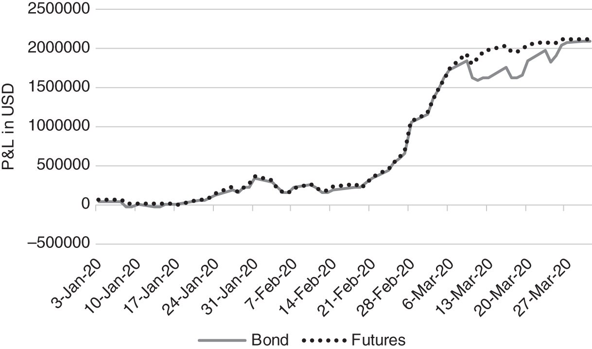
FIGURE 9.4 Evolution of the Treasury and of the hedging futures portfolio
Source: Authors
During March, there was a period of larger discrepancies: For example, at the end of the reference quarter of the Dec 19 contract (when the rebalancing from Table 9.1 was calculated), the hedge portfolio established on Jan 2, 2020, and maintained without adjustment had suffered a loss of USD 1,959,518, while the note had returned a profit of USD 1,631,250, resulting in a loss of the hedged position of USD 328,268. This corresponds to about 20% of the overall move.
Investigating the reasons for the poor performance of the hedge during this period, with the asset swap spread (using a swap with SOFR as floating leg) of the Treasury note becoming more positive, it appears as if its pricing has been ephemerally influenced by the corporate bond market. Hence, the foundation of the whole hedging concept of constant spreads (Figure 9.1) has been violated. As a consequence, the markets, which should be linked by the argument at the beginning of this chapter, have decoupled, and thus the hedge based on the assumption of constant asset swap spreads has not performed as well as before. This example can also serve as illustration of the risk of mis-hedging with futures strips if the fundamental link does not hold, for example, when applied to a corporate bond or in times of changes in the effect of capital costs on the relative pricing between futures and government bonds.
Putting a happy ending to the story, the decoupling turned out to be ephemeral indeed, and by the end of March, the gap was closed again. For example, on Mar 31, 2020, the bond had gained USD 2,100,000 versus a loss on the future portfolio of USD 2,113,099, bringing the mismatch down to less than 1%. If confirmed by a larger number of cases, the experience of this example points to two conclusions:
- This approach to hedging seems to work in practice as long as its theoretical foundation (Figure 9.1) holds firm. When the foundation shakes, for example, due to changes in the leverage situation driving the asset swap spreads (with SOFR as floating leg) of government bonds away from zero, the hedge built on it is also at risk.
- If mismatches of the hedge are considered to be ephemeral, a hedger could simply maintain it and wait for the discrepancy to disappear, as in this example. And a relative value trader might even consider the brief periods as arbitrage opportunities in the framework of the links between the three markets from Figure 9.1: Buying the bond versus selling the hedge portfolio of futures on Mar 18, 2020, at a spread of USD 328,268 would have returned a profit of USD 315,169 until Mar 31, 2020. Obviously, this “arbitrage” is based on the condition of the foundation holding and the mismatches being short-lived.
Regarding the implementation of these hedges in software programs, Excel worksheets are not practical for recalculating the hedge ratio every day, let alone for managing a whole portfolio of hedges or for monitoring the market for a large number of potential arbitrage opportunities. Readers should therefore budget time and money for the IT-implementation and back-testing both of the possible approaches to hedging described here and of alternatives which may fit better to their specific goals.
NOTES
- 1 Being OTC instruments, of course other agreements are possible as well.
- 2 For the goal of an overall comparison, these simplifications seem acceptable. For the specific hedge example below, we will use the actual reference quarters.
- 3 Assuming money market conventions for discounting and bond conventions for the fixed payment, i.e., without adjusting the quarterly coupon payments for the actual length of the reference quarters.
- 4 The formula in Burghardt, Belton, Lane et al. (1991) seems to apply bond conventions for discounting, which would result in the present value of the floating side being different from 100 and may need to be corrected.
- 5 Being OTC products, there are no firm specifications like for future contracts. Hence, we need to base our statements on sources from clearinghouses like CME (Q4 2018) or https://www.cmegroup.com/trading/interest-rates/cleared-otc.html and anecdotal evidence.
- 6 Apart from FOMC meetings, a quarter end may be considered as problematic. On the other hand, the SRF (discussed in Chapter 1) could be seen as mitigating this problem.
- 7 Using the method presented in the sheet “Strips,” which is not encoded again in this sheet.
- 8 Using the adjustment for the known SOFR values during the reference quarter for the first future and the techniques for accounting for FOMC meetings during the reference quarter of the last future once more (see Figure 9.3).
- 9 Also in this case, the implied daily SOFR values were almost the same as the future rate.
- 10 Keep in mind that the simple multiplication of the number of contracts (717) with the BPV (USD 25) does not work for the 101 front-month contracts. Hence, the P&L of the hedge portfolio is obtained by (717 – 101) * 25 plus 101 * 0.8384 * 25 (see cell N3).
- 11 For ease of comparison, the P&L of long positions in both the note and the futures strip are depicted; of course, in the actual hedge, a long position in the bond is hedged with a short position in the futures strip, as shown in Table 9.1.