
CHAPTER 2
SOFR Futures
While three-month Eurodollar futuresuline{a} settle to a three-month term rate at the end of the contract, SOFR futures settle to the average of an overnight rate during the last three months prior to the expiration of the contract – referred to as the reference period of the contract. Despite this difference, SOFR futures share several characteristics with Eurodollar futures, since prior to entering the reference period both contracts are functions of the forward rate associated with the reference period. As a result, Eurodollar futures and SOFR futures represent consecutive three-month forward segments of the yield curve – for unsecured borrowing in the case of Eurodollars and for secured borrowing in the case of SOFR. It follows that we can apply many of the same analytic techniques to SOFR futures that have been developed for Eurodollar futures.
Accordingly, this chapter starts by describing the specifications for 3M SOFR futures (SR3), before showing how analytic approaches common to the Eurodollar complex can be applied after the migration to SOFR. It then adds 1M SOFR futures (SR1) and analyzes the spread between 3M and 1M SOFR futures. Finally, it outlines more advanced modeling and hedging techniques via processes, again by building on the work done for LIBOR products.1
However, once the reference period of a SOFR futures contract begins, the aggregative function stops, and we must keep track of each of the overnight rates that span the reference period, as illustrated in Figure 2.1. Readers should keep this break in mind whenever considering SOFR futures and options. As soon as the reference period of a SOFR future starts, one does not deal with a LIBOR-like aggregation of daily rates into a forward term rate anymore but rather, with a collection of already-known and still unknown daily SOFR values. This difference means that the front-month SOFR futures contract requires extra attention and new analytic approaches. Fortunately, in the case of futures, the necessary adjustments of terminology and analyses are rather simple, and this chapter offers some suggestions for strips and rolls. In the case of options on futures on the other hand, this conceptual difference will result in path-dependent Asian options and confront us with a much bigger challenge, as we'll see in Chapter 5.
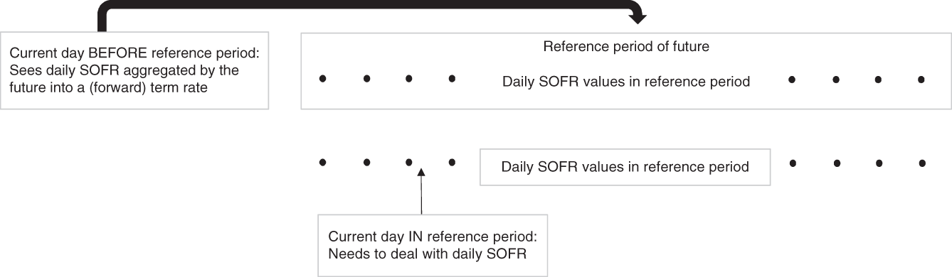
FIGURE 2.1 The aggregation of daily SOFR via the future before the reference period starts
Source: Authors
3M SOFR FUTURES: CONVENTIONS
The key difference between a Eurodollar (ED) and a three-month SOFR (SR3) future is the fact that the underlying rate of the former is a traded, forward-looking, unsecured term rate, while the settlement rate of the latter needs to be calculated from overnight rates for secured borrowing and lending and is therefore by nature backward-looking. The basis between unsecured and secured borrowing will be analyzed in Chapter 4. Here we focus on the implications of the difference between forward-looking and backward-looking rates on the conventions of the futures. In order to account for this difference, as a first step, we need to adjust the terminology used to describe the contract month:
- The “Sep 2022 ED” future ends trading and settles in Sep 2022 on a 3M LIBOR rate, which begins in Sep 2022 and matures in Dec 2022.
- The “Sep 2022 SR3” future ends trading and settles in Dec 2022 to a (modified) geometric average of daily SOFR rates observed during a period, which begins in Sep 2022 and ends in Dec 2022.
Hence, while the underlying rates of a “Sep 2022” ED and SR3 future cover almost2 the same period, end of trading and settlement occur in a SR3 future at the end rather than at the beginning of this period. This is a result of the different nature of the underlying rates: 3M LIBOR is a traded forward-looking term rate, while the 3M SOFR settlement rate needs to be constructed by looking back at the traded overnight SOFR during the past 3M. While even at the last day of trading of an ED contract, the underlying rate refers to a period completely in the future, at the last day of trading of an SR3 contract, the underlying rate refers to a period in the past, which is therefore completely known (except for the very last overnight rate, which is published on the business day after the last trading day). Consequently, during the last three months of the life of an SR3 contract, more and more of the rate determining its settlement price becomes known, typically resulting in reduced volatility – unlike in ED futures.
We will analyze these economic consequences below; for the moment, we focus on the consequences for terminology and conventions: The contract month (e.g., Sep 2022) of an SR3 future refers to the reference quarter (e.g., Sep 2022 to Dec 2022) of the following three months, whose SOFR will be used to calculate the settlement price at the end of the reference quarter, i.e., three months after the “contract month.” While an ED contract ends trading when the underlying rate (the forward-looking 3M LIBOR) begins, the SR3 contract of the same “contract month” ends trading three months later, when all overnight SOFR values of the reference quarter (except the last one) and thus the term rate for settlement is (almost) known.
Using this adjustment in terminology, the conventions of ED contracts have been closely mirrored in those of SR3 contracts, as summarized in Figures 2.2 and 2.3. Crucially, the calculation of the settlement price uses ISDA compounding with Act/360 as the daycount convention.
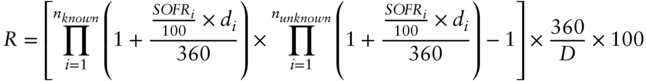
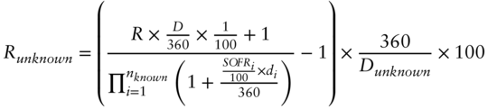
The formula for the settlement price of an SR3 futures contract is defined as 100 less the settlement rate, R, given by the equation
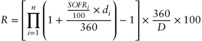
where
- n is the number of business days (for US government securities) during the reference quarter.
- SOFRi is the SOFR for day i
(published on the next business day). In keeping with CME's conventions, the %-value of SOFR is entered (e.g., 1.5 for a SOFR of 1.5%), hence the factor 1/100.
Delivery months Nearest 39 March Quarterly months (Mar, Jun, Sep, Dec) Reference quarter Begins on 3rd Wed (included) of 3rd month preceding the delivery month
Ends on 3rd Wed (excluded) of the delivery monthContract month Month in which the reference quarter begins Last trading day Exchange business day preceding 3rd Wed of the delivery month Delivery Cash settlement
First business day after last trading day, i.e., usually 3rd Wed of the delivery month
(This is the day the Fed publishes SOFR for the last trading day)Settlement rate Compounded SOFR realized during reference quarter (see formula in text)
Rounded to the nearest 0.01 bpSettlement price 100 minus settlement rate Online resource https://www.cmegroup.com/markets/interest-rates/stirs/three-month-sofr.contractSpecs.html FIGURE 2.2 SOFR futures: settlement calculations
Source: Authors, based on CME
Contract size USD 25 per basis point per annum Minimum price increment 0.25 basis points per annum 0.5 basis points per annum
for contracts with 4 months or less until last day of trading for other contracts
Trading venues and hours CME Globex and CME ClearPort: 5pm to 4pm, Sun-Fri Block trade minimum size 250 contracts Asian Trading Hours (4pm–12am, Mon-Fri on regular business days and at all weekend times) 500 contracts European Trading Hours (12am– 7am, Mon-Fri on regular business days) 1000 contracts Regular Trading Hours (7am–4pm, Mon-Fri on regular business days) Product codes SR3 CME SFR Comdty Bloomberg FIGURE 2.3 3M SOFR futures: technical specifications
Source: Authors, based on CME
Delivery months Nearest 13 calendar months Last trading day Last exchange business day of the delivery month Delivery Cash settlement First business day after last trading day (This is the day the Fed publishes SOFR for the last trading day) Settlement rate Arithmetic average of SOFR realized during delivery month (Average is taken over calendar days, not business days) (For non-busines days, the SOFR of the preceding business day is used) Rounded to the nearest 0.1 bp Settlement price 100 minus settlement rate Online resource https://www.cmegroup.com/markets/interest-rates/stirs/one-month-sofr.contractSpecs.html FIGURE 2.10 1M SOFR futures: settlement calculations
Source: Authors, based on CME
Contract size USD 41.67 per basis point per annum Minimum price increment 0.25 basis points per annum 0.5 basis points per annum
during delivery month before delivery month
Trading venues and hours CME Globex and CME ClearPort: 5pm to 4pm, Sun-Fri Block trade minimum size 125 contracts Asian Trading Hours (4pm–12am, Mon-Fri on regular business days and at all weekend times) 250 contracts European Trading Hours (12am– 7am, Mon-Fri on regular business days) 500 contracts Regular Trading Hours (7am–4pm, Mon-Fri on regular business days) Product codes SR1 CME SER Comdty Bloomberg FIGURE 2.11 1M SOFR futures: technical specifications
Source: Authors, based on CME
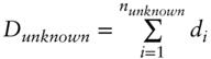
- di is the number of calendar days for which SOFRi is used.
Until the next business day, the SOFR for the previous business day is used, e.g., on weekends and holidays. Thus, if Friday and Monday are business days, the SOFR for Friday (published on Monday) is used for Friday, Saturday, and Sunday, and the corresponding di is 3.
- D is the total number of calendar days during the reference quarter, i.e.,
 .
.
The Excel sheet “3M versus 1M” accompanying this chapter implements these calculations for the Sep 2022 SR3 contract. The reader can define the SOFR either manually for each day during the reference quarter or set an SOFR level and slope for the whole reference quarter and observe the impact on the settlement price.
As outlined in Chapter 1, the Fed may revise SOFR published in the morning. If such a revision occurs for the SOFR of the last day of the reference quarter, it cannot be reflected in the settlement price of the future, which CME determines in the morning of the delivery day. By contrast, revisions for all other SOFR are taken into consideration for calculating the settlement rate (CME May 2018, p. 6).
Figure 2.4 illustrates the situation of SR3 contracts during the reference quarter: At the “current” day during the reference quarter, the SOFR values for the past period of the reference quarter are known, while the SOFR values for the future period of the reference quarter are not. Hence, as the “current” day progresses through the reference quarter, the share of known versus unknown values determining its settlement rate increases. This is similar to the situation in FF (Fed Funds) contracts, but different from the situation for ED contracts.
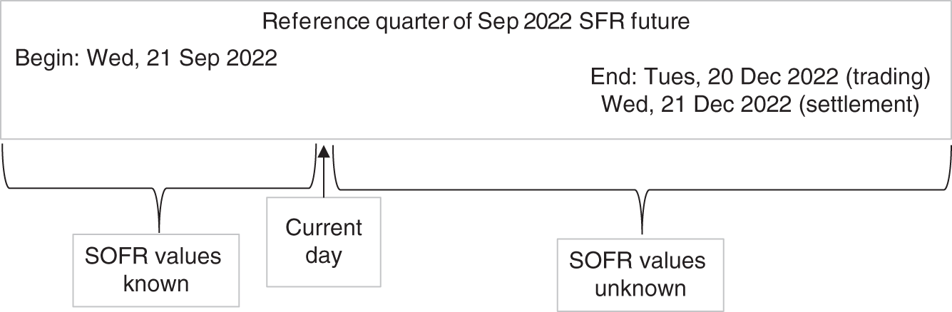
FIGURE 2.4 SOFR futures during reference quarter
Source: Authors
This is also the reason for the behavior seen in Figure 2.5, which shows the history of all SR3 future prices.3 As SR3 contracts approach their end, an increasing portion of their settlement rate is known, and hence:
- Their volatility tends to decrease, as seen in the lines becoming flatter toward their end.4
- They respond less and less to changing market expectations about future interest rates. During the decreasing interest rate environment of 2019, expectations about Fed rate cuts affected all SOFR values in the reference quarters of back month contracts, but only some of the SOFR values in the reference quarter of the front month contract, which therefore tended to stick to a higher level.
Abstracting from this conceptually different behavior of front month SR3 futures, Figure 2.5 reflects the evolution of the market consensus of Fed policy over time. After a rather parallel curve shift down in 2019 and a flat curve around zero in 2020, the relatively steep curve of 2021 implies a long period of gradual rate hikes. This analysis is familiar from other future markets, since the Fed policy drives both secured (SOFR) and unsecured (ED) rates underlying future contracts.
One can therefore conclude that, with the exception of the front month contract, the transition from LIBOR to SOFR is little more than a renaming exercise for the futures market. This is a contrast to the problems this transition faces in cash loan markets, which will be described in the next chapter, and in option markets, which will be covered in Chapter 5. The similarity of conventions between 3M SOFR and ED contracts also facilitates the migration: Since LIBOR will end on June 30, 2023, ED futures expiring after this date will settle on a fallback clause, described in more detail in Figure Intro.1 and on https://www.cmegroup.com/education/files/webinar-fallbacks-for-eurodollars.pdf.
An important consequence of ED contracts after June 30, 2023, being spreads over a secured rate is that past this date only FF futures will trade on an unsecured rate. From mid-2023 onward, the unsecured–secured basis can therefore only be traded by SOFR–FF spread contracts, not by the currently more liquid SR3:ED spread futures anymore. The implications for analysis and positioning will be discussed in Chapter 4.
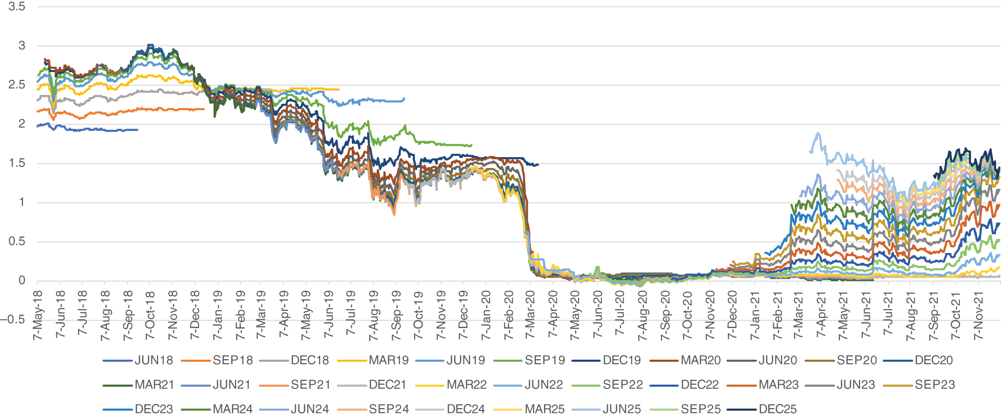
FIGURE 2.5 SOFR future price history
Source: Authors, from data provided by CME
3M SOFR FUTURES AS MARKET PRICES FOR CONSECUTIVE 3M FORWARD SOFR
The similarity of conventions between 3M SOFR and ED contracts, which facilitates the migration of trading after the end of LIBOR, also facilitates the migration of analytic concepts from the unsecured to the secured yield curve.
The importance of ED futures for yield curve analysis is based on the fact that they provide market prices for consecutive 3M forward periods of their underlying unsecured (LIBOR) rate – after adjusting for biases such as convexity. This is the foundation for many important analyses, such as:
- Using ED futures as building blocks for (forward) LIBOR rates via strips.
- The other way around, decomposing LIBOR rates into their individual 3M forward components and hedging them via futures (Burghardt et al. 1991).5
- Assessing the carry, rolldown, and risk/return of different parts of the yield curve and in different macroeconomic scenarios.6
- Extracting constant maturity zero or par rates, e.g., via spline models (Huggins and Schaller 2013, chapter 11), which are the basis for many further analyses.
The switch from LIBOR to SOFR as reference rate necessitates the transfer of this arsenal of analytic methods from the unsecured to the secured yield curve – and the proximity of ED and SOFR future conventions enables a straightforward transfer. While a complete treatment of secured yield curve analysis is outside the scope of this book, it offers a few examples of this transfer, specifically in this chapter for the secured yield curve and in Chapter 5 for the secured volatility curve, and focuses on its practical implications for hedging and trading in section 2. Chapter 6 discusses the different biases, such as convexity, in ED and SOFR contracts. As it turns out that there are no biases from nonlinearities in 3M SOFR futures, extracting secured forward rates from SOFR contracts is easier than extracting unsecured forward rates from ED contracts.
In fact, Figure 2.5 depicts the market prices for consecutive 3M forward periods of the secured yield curve. Slicing through the data in two dimensions, one can extract the historical evolution (one dimension) of the market expectations about the secured rate at different forward dates (second dimension). Figures 2.6 and 2.7 present the perspectives from these two dimensions.7 The result confirms the similarity to pictures familiar from the unsecured yield curve: Expectations about Fed cuts led to an inversion of the curve from 2018 to 2019; the anticipation of low rates for a prolonged period of time is reflected in the compressed forward curve close to zero during 2020, while speculation about rate hikes led to more differentiation during 2021 again. One could now use these data as input into further analyses not performed here, for example, a macroeconomic analysis of the mismatches between the market consensus and actual Fed policy8 or a relative value search for mispricings (e.g., opportunities for butterflies).
This analysis will be repeated in Chapter 5 to extract the evolution of the realized volatility in different parts of the forward curve for the secured rate. Both analyses can then be combined to assess the historical average and distribution of risk/return (e.g., Sharpe ratios, across the secured yield curve). This is an example of the transfer of established analysis techniques from the unsecured curve. In all these examples, readers should keep in mind the structural break due to the introduction of the Fed's standing repo facility (discussed in Chapter 1), which also affects statements based on the data from Figure 2.5. Readers also should repeat the analyses with post-SRF data exclusively once a sufficient amount of such data is available.
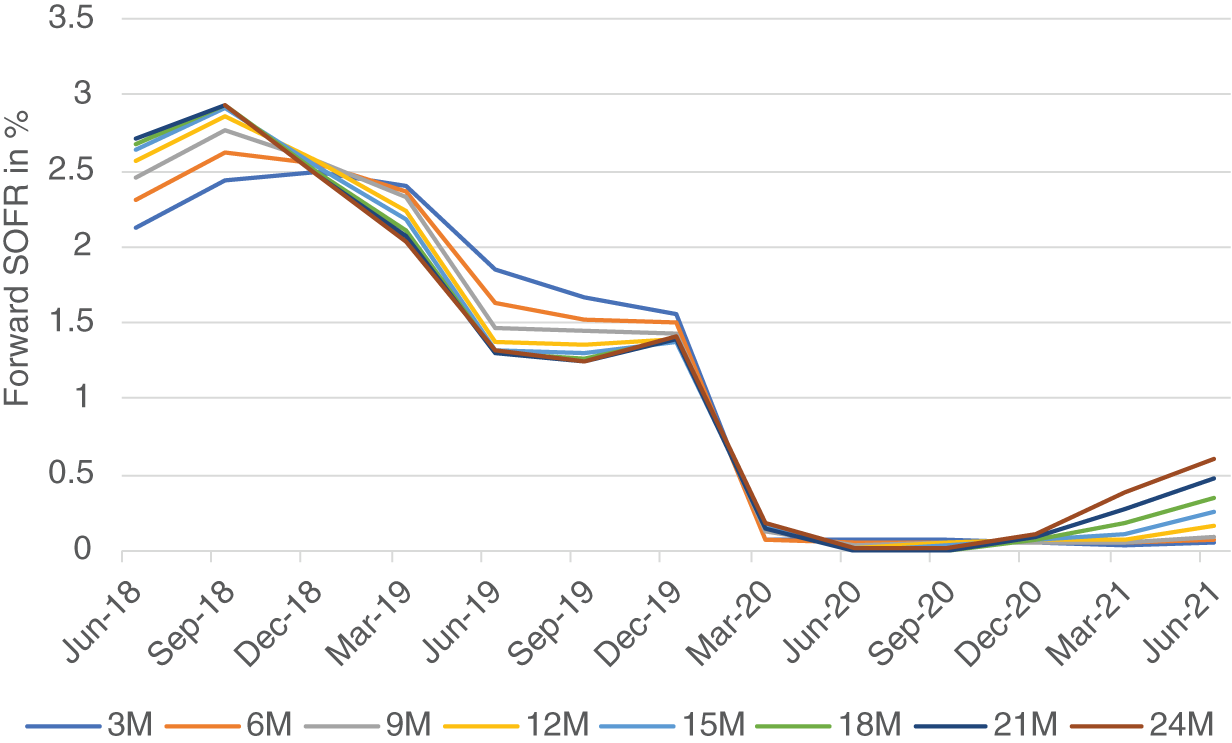
FIGURE 2.6 Consecutive 3M forward rates of the secured yield curve as implied by 3M SOFR futures
Source: Authors, from CME data
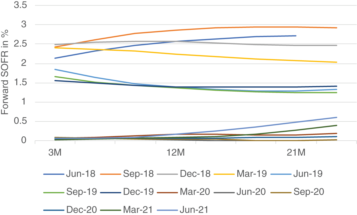
FIGURE 2.7 Consecutive 3M forward rates of the secured yield curve as implied by 3M SOFR futures
Source: Authors, from CME data
3M SOFR FUTURES: STRIPS
Since SR3 futures represent consecutive 3M forward interest periods (even without adjusting for nonlinearities as in case of ED futures), they can be easily combined into longer tenors. For example, buying the Sep 2022 and Dec 2022 SR3 futures on Sep 21, 2022, i.e., the beginning of the reference quarter of the Sep 2022 contract, gives exposure to the 6M interest period of all daily SOFR values during the reference quarters of both contracts.
This combination of successive ED futures is known as a strip and the corresponding interest rate as a strip rate (Burghardt et al. 1991, p. 86). It is a simple method to calculate term rates from the future markets; the example above corresponds to the 6M term rate implied by the futures market. However, when the term does not match the reference quarters, the results could be distorted. Imagine we want to calculate a 5M SOFR term rate from the Sep 2022 and Dec 2022 SR3 futures contract on Sep 21, 2022, and that the market expects a Fed rate hike on Mar 1, 2023. This expectation would probably be reflected in the Dec 2022 SR3 price but should not affect the 5M term rate, which ends before Mar 1, 2023. Consequently, the simple method of calculating term rates from future markets via strips works well if the term matches the reference quarters (and in case of relatively constant forward SOFR during the reference quarter of the last future in the strip) but needs to be adjusted for the shape of the forward curve during the last reference quarter if it exceeds the term. We will address this issue later in this chapter.
When applying the concept of strip rates to the SOFR futures market to calculate term rates starting today, one needs to keep in mind the difference between front-month SOFR and front-month ED futures contracts, depicted in Figure 2.4:
- For ED strips, the first contract used in the strip covers an interest period entirely in the future. Hence, the time from today until the interest period covered by ED futures needs to be taken from the spot money market. For example, for a term rate starting on Sep 1, 2022, for the time until Sep 21, 2022, the 3W LIBOR is used.
- For SR3 strips, the first futures contract used in the strip covers with its reference quarter an interest period that is partly in the past and partly in the future. Hence, unlike for ED strips, it is not necessary to refer to the spot money market. In the example above, for a term rate starting on Sep 1, 2022, for the time until Sep 21, 2022, the price of the Jun 2022 SR3 contract can be used. However, it needs to be adjusted for the SOFR values already observed during the part of the reference quarter before Sep 1, 2022.
This difference is illustrated in Figure 2.8.
To calculate the yield for the period until the first full reference quarter from the front month SR3 contract, one needs to split its reference quarter into known and unknown SOFR values (Figure 2.4), i.e.,
One can then solve for the interest rate implied by the front month SR3 contract for the unknown period of its reference quarter. Conceptually, this can be considered as extracting the implied interest rate for the unknown period from the future price (combining the known and unknown periods) and the SOFR values already known.
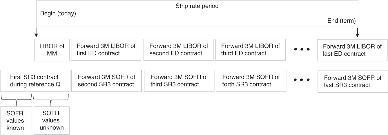
FIGURE 2.8 Calculating strip rates from ED and SR3 futures
Source: Authors
where (in addition to the variables from the formula above)
- R is the rate implied by the front month SR3 contract, i.e., 100 minus its price.
- D is the total number of calendar days during the reference quarter, i.e.,
 .
. - Dunknown is the total number of calendar days during the unknown (future) part of the reference quarter, i.e.,
 .
.
Using this rate calculated from the front month SR3 contract (rather than a LIBOR money market rate) for the first “short” interest period until the first “full” 3M reference quarter is the only conceptual adjustment required. Otherwise, strip rates can be calculated from SOFR futures in the same manner as from ED futures, i.e.:
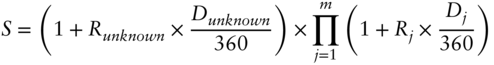
where
- S is the strip rate.
- m is the number of SR3 contracts used after the front month contract (which is used for calculation of Runknown).
The last day of the term of the strip rate falls in the reference quarter of the mth future.
- Rj is the rate implied by the price of the jth SR3 contract, i.e., 100 minus its price.
- Dj is the total number of calendar days during the reference quarter of the jth SR3 contract for j < m and the number of calendar days during the reference quarter until the term of the strip rate for j = m.
This calculation corresponds to compounding all daily SOFR values as implied by the SOFR future prices during the term of the strip. Using money market conventions, the strip rate S can then be annualized by solving the following equation for Sann:
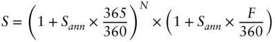
where
- Sann is the annualized strip rate using money market conventions.
- N is the number of whole years in the term of the strip.
- F is the number of days in the term of the strip minus N years.
The Excel sheet “strip” accompanying this chapter illustrates these calculations for the example of a 6M strip rate starting on Oct 3, 2022. Assuming hypothetical daily SOFR values of 95 bp for the known period of the reference quarter of the Sep 2022 contract and futures prices of 99, 98.5, and 98 for the three SR3 contracts in the strip (the user can change these numbers), in a first step the known SOFR values are compounded, just like when calculating the settlement rate (cell E13). Together with the price of the Sep 2022 contract, this allows determining the value Runknown (cell G7). Then, the Dj's are calculated, with the last one corresponding to the number of days from the start of the reference quarter of the Mar 2023 contract (Mar 15, 2023) to the end of the 6M term (Apr 3, 2023). Applying the formula above, the strip rate is determined (cell G9) and annualized (cell G10).9 For the hypothetical values above, the annualized 6M strip rate is thus 1.34%.
3M SOFR FUTURES: ROLLS
We have already stated that the transition from ED to SOFR futures is basically a renaming exercise for back-month contracts, but not for front-month contracts during the reference quarter (see Figures 2.1 and 2.4). As a result, the transition has a significant effect on the roll from front-month into back-month contracts. Taking into account the increasing decoupling of front-month SOFR futures from the overall market during their reference quarter, which results in the reduced volatility and “stickiness” observed in Figure 2.5, it seems advisable to execute the roll before SOFR futures enter their reference quarter. Using the example of the Dec 19 SR3 future, which experienced a sharp drop of SOFR during its reference quarter, the roll into Mar 20 would have cost 138 bp if executed at the end of its reference quarter, but only 4 bp if executed at its beginning. Of course, this is a relatively extreme case, but Figure 2.9 suggests10 that rolling at the beginning rather than at the end of the reference quarter has been better (i.e., closer to zero) in almost every circumstance.
This means that, for SOFR contracts, the roll should not be executed between front-month and back-month contracts, as usually done with ED futures, but between second and third listed contracts.
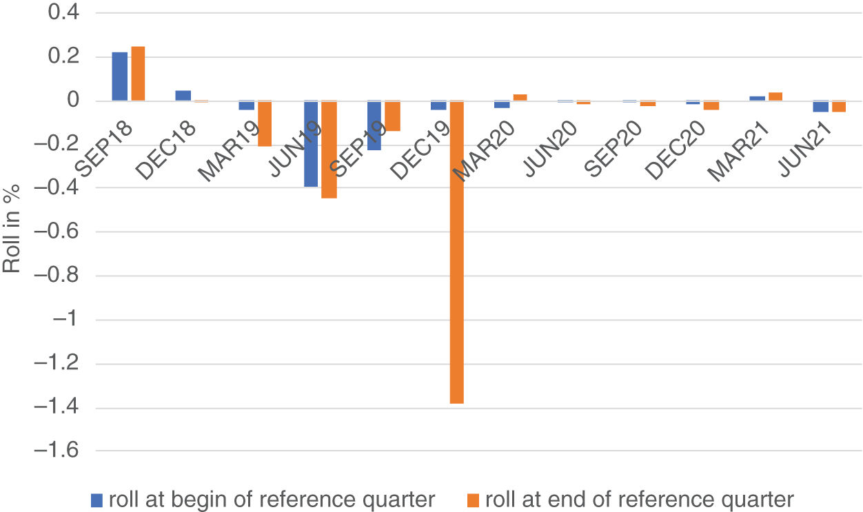
FIGURE 2.9 Rolls for past 3M SOFR futures
Source: Authors, from CME data
1M SOFR FUTURES: CONVENTIONS
As the conventions of 3M SOFR futures (SR3) closely mirror those of Eurodollar (ED) contracts,11 the conventions of 1M SOFR futures (SR1) have been modeled along the lines of Fed Funds (FF) contracts, as summarized in Figures 2.10 and 2.11. Crucially, the calculation of the settlement price uses a simple arithmetic average over the calendar (not business) days of the delivery month, which is also the stated contract month. As with SR3 futures, the SOFR value for the previous business day is used on each subsequent calendar day up until the next business day. In the example of the Oct 2022 SR1 contract illustrated in the Excel sheet “3M versus 1M,” for the two first days of the contract month, Saturday, 1 Oct 2022, and Sunday, 2 Oct 2022, the SOFR value from Friday, 30 Sep 2022 (published on Monday, 3 Oct 2022), will be used. The settlement rate is then calculated by dividing the sum of the SOFR values for each calendar day by the number of calendar days in the contract month.
The similarity of conventions between SR1 and FF contracts has two important implications:
- The simple, arithmetic average used in the SR1 contract does not reflect the conventions of most SOFR-related instruments. For example, if one repeatedly rolled a cash balance overnight earning the daily SOFR value, the balance on any given day would reflect daily compounding (i.e., the geometric average) rather than the simple, arithmetic average used in the 1M SOFR contract. As a result, there is a risk that liquidity would be split between the two conventions, to the detriment of the SOFR complex generally. In addition, this also further complicates the pricing of options on 1M SOFR futures because there are formulae for geometric but not for arithmetic Asian options. (See Chapter 5.)
- An advantage is that the spread between SR1 and FF futures is not driven by different specifications, but (almost) only by the basis between secured and unsecured lending. This results in the spread contracts being a clean reflection of the market price for that basis. Hence, the fair value of the spread contracts can be determined via the basis. Likewise, the basis, which features in many relative value relationships, can be cheaply and easily traded via listed spread contracts. (See Chapter 4.)
1M VERSUS 3M SOFR FUTURES
In contrast to trading SR1 versus FF futures, trading SR1 versus SR3 futures does not include exposure to a basis (as both have the same underlying secured rate) but exposure due to their different specifications. As such, spread trades between SR1 and SR3 do not depend on the secured–unsecured basis but mainly on two factors:
- As they cover different time periods, the spread depends on the yield curve and hence on its driving factors, such as Fed policy.
- As they use different specifications, the spread also depends on the mathematical formulas for determining final settlement prices, in particular, the difference between a simple average and daily compounding.
The effect of the first factor, different time periods, can be minimized by constructing spread trades with a good overlap. Specifically, one can trade a SR3 contract versus the two SR1 futures in the middle of its reference quarter. For example, the Sep 2022 SR3 future, with a reference quarter from Wed 21 Sep, 2022 to Wed 21 Dec, 2022, can be traded versus Oct 2022 and Nov 2022 SR1 futures. The relationship of the time periods covered is illustrated in Figure 2.12.
Since the overlap is good but not perfect, some exposure to the underlying yield curve remains:
- Parallel curve shifts only affect the SR1–SR3 spread via the mathematical issues described below, not via different time periods.
- The slope of the yield curve affects the SR1–SR3 spread also via the different time periods. While the construction shown in Figure 2.12 minimizes the impact, it should be noted that the time period covered by the two SR1 contracts is not precisely in the middle of the reference quarter. Actually, the precise position depends on the position of the third Wednesday in the contract month. In the example of Sep 2022 (which was chosen with the goal of illustrating this effect), the third Wednesday is late in the contract month (Sep 2022), and therefore a larger portion at the end than at the beginning of the reference quarter is not covered by the SR1 contracts. Thus, a steepening of the yield curve will affect the SR3 contract more, supporting a cheapening of SR3 versus SR1. This explains the impact of the curve slope on the theoretical spread shown in Table 2.1.
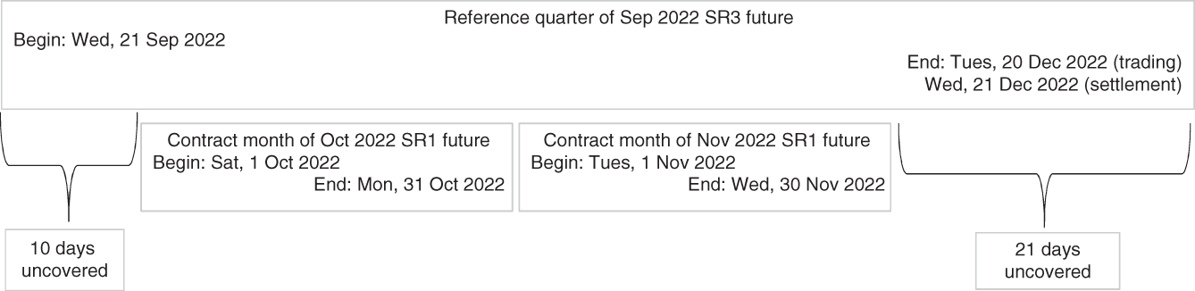
FIGURE 2.12 Time periods covered by 1M and 3M SOFR futures
Source: Authors
- Moreover, jumps in SOFR during the period of the reference quarter not covered by SR1 futures can have a strong effect on the spread. For example, a Fed rate hike on Dec 1, 2022, by 50 bp, driving the SOFR from 10 bp to 60 bp, results in a fair value for the SR1–SR3 spread of 12 bp.12 By changing the values in the excel sheet “3M versus 1M,” the reader can assess the impact of different scenarios of the SOFR evolution during the reference quarter on the fair value of the spread between the 1M and 3M SOFR contracts.
TABLE 2.1 Fair value of Sep 2022 SR1–SR3 spread
Source: Authors
| SOFR at begin of reference quarter (bp) | SOFR slope during reference quarter (bp) | Settl. Price Sep 2022 SR3 | Settl. Price Oct 2022 SR1 | Settl. Price Nov 2022 SR1 | Fair Value of Spread Contract (bp) (CME convention) |
|---|---|---|---|---|---|
| 0 | 0 | 100.00 | 100.00 | 100.00 | 0.00 |
| 0 | 25 | 99.88 | 99.93 | 99.85 | 1.33 |
| 0 | 50 | 99.75 | 99.86 | 99.69 | 2.67 |
| 100 | −50 | 99.25 | 99.14 | 99.31 | −2.59 |
| 100 | −25 | 99.12 | 99.07 | 99.15 | −1.24 |
| 100 | 0 | 99.00 | 99.00 | 99.00 | 0.12 |
| 100 | 25 | 98.87 | 98.93 | 98.85 | 1.49 |
| 100 | 50 | 98.75 | 98.86 | 98.69 | 2.85 |
| 500 | −50 | 95.22 | 95.14 | 95.31 | 0.15 |
| 500 | −25 | 95.09 | 95.07 | 95.15 | 1.62 |
| 500 | 0 | 94.97 | 95.00 | 95.00 | 3.11 |
| 500 | 25 | 94.84 | 94.93 | 94.85 | 4.59 |
| 500 | 50 | 94.72 | 94.86 | 94.69 | 6.09 |
| ICS (Inter-Commodity Spread) | Between SR3 and the two SR1 fully in its reference quarter (e.g., between Sep 2022 SR3 on one hand and Oct 2022 SR1 and Nov 2022 SR1 on the other hand) |
| Weighting | Three SR1 each versus ten SR3, resulting in almost equal BPV |
| Price display | Average of the two SR1 prices minus SR3 price (e.g., (Oct 2022 SR1 + Nov 2022 SR1) / 2 - Sep 2022 SR3) |
| Last trading day | Equal to the last trading day of the first of the two SR1 contracts contracts |
| For other specifications, refer to Table 04.01 | |
FIGURE 2.13 1M–3M SOFR spread futures: specifications
Source: Authors, based on CME
The CME lists 1M–3M SOFR spread futures constructed according to the idea of overlapping time periods illustrated in Figure 2.12 and to achieve (almost) neutrality in basis point values (BPV).13 Figure 2.13 summarizes their specifications. The key is the weighting, corresponding to three SR1 contracts each versus 10 SR3 contracts, almost netting out the BPV (6*41.67 = 250.02). The remaining BPV difference explains the difference between spreads calculated via the actual contracts and via the CME convention. However, this difference is less than 1 bp; accordingly, the Excel sheet and Table 2.1 show the spreads according to the CME convention only.14
Despite the (almost) BPV-equal weighting of 1M and 3M SOFR futures in the CME spread contract, there remains exposure to the slope of the yield curve due to time periods that do not perfectly overlap (as discussed above) and even to parallel curve shifts through different conventions. When SOFR is equal to zero, there is no difference between a simple, arithmetic average and daily compounding. But as SOFR rises, the difference becomes more important and reaches 3 bp for a constant SOFR at 5% during the reference quarter.
Table 2.1 shows the fair value of the 1M–3M SOFR spread (calculated from the Excel sheet) for different scenarios of SOFR during the reference quarter of the Sep 2022 SR3 future. Due to the reasons described above, at low interest rate levels and a flat curve, the fair value is small – which could explain the current illiquidity of the spread contracts. On the other hand, the spreads become more meaningful when rates rise (due to the different conventions) and when the yield curve exhibits a shape (due to different time periods covered). In general, the higher the level and the steeper the slope of SOFR during the reference quarter, the higher the fair value of the spread. Hence, it is possible that liquidity in spread trading will increase with (speculation about) Fed rate hikes. Depending on the timing (see the hypothetical example of a Fed hike on Dec 1, 2022), the spread contracts could provide an attractive capital-efficient way to trade expectations about Fed policy.
1M AND 3M SOFR FUTURES: LIQUIDITY
Figures 2.14 and 2.15 show histories for volume and open interest for 1M and 3M SOFR contracts. Both on an absolute scale and relative to other newly introduced futures, SOFR contracts got off to an impressive start. Although there has been some concern about insufficient liquidity during the discussion about basing a term rate on SOFR futures,15 the recent almost exponential rise in the liquidity for SR3 contracts is probably a good enough response to this concern.
Comparing both SOFR futures, while 1M contracts had a better start, only 3M contracts have benefited from the recent strong increase in liquidity. Actually, it appears as if liquidity might have started to concentrate in SR3 futures.
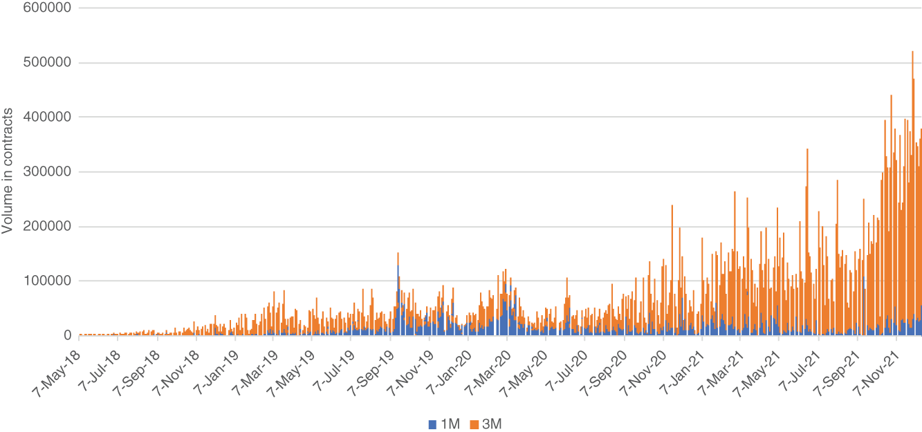
FIGURE 2.14 SOFR future daily volume
Source: Authors, from data provided by CME
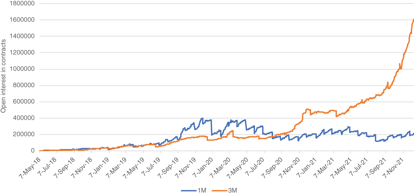
FIGURE 2.15 SOFR future open interest
Source: Authors, from data provided by CME
However, we think it is too early to “call the race” and will find in the following chapters some factors that are likely to impact the future liquidity situation of SOFR futures in general and the distribution between SR1 and SR3, including:
- The share of simple versus compound conventions of SOFR-based cash loans and securities will have an effect on the demand for hedging products with the same convention. Hence, the move toward using compounding for SOFR floating rate notes (FRNs) following ARRC's recommendation and model language could be one factor supporting the recent concentration of liquidity in 3M SOFR contracts. And the potential issuance of a Treasury SOFR FRN could further reinforce this trend. (See Chapter 3.)
- As SR3:ED spread futures give the biggest exposure to the secured–unsecured basis, demand and hence liquidity is highest for this spread (see Chapter 4). However, following the end of LIBOR in June 2023, the SR3:ED spread will disappear as a source for exposure to this basis. After this date, only the SR3:FF and SR1:FF spread futures cover the secured–unsecured basis. And among these two, SR1:FF provides the “cleaner” exposure to the basis, while SR3:FF is also subject to different time periods and conventions. Hence, one may expect the end of LIBOR to result in a boost in demand for 1M SOFR futures since SR1:FF could well become the best product to trade the secured–unsecured basis, as described at the end of Chapter 4.
- Liquidity in futures is influenced by liquidity in the options on futures (and vice versa). And the impressive liquidity in SR3 futures was achieved despite a lack of liquidity in its options. One can therefore expect another boost in liquidity for SR3 contracts when liquidity in options on 3M SOFR futures increases (despite the remaining challenges outlined in Chapter 5) – for example, due to migration from options on ED futures, hedging floored or capped SOFR loans, or the opportunities to trade options on SR3 and ED futures versus each other.
1M AND 3M SOFR FUTURES: ASSESSING THE EFFECT OF FOMC MEETINGS
Given the importance of Fed policy for the short end of the curve, analyzing and immunizing SOFR future positions against the exposure to policy rate changes is a key consideration:
- For 1M futures, the impact is easy to calculate: A rate hike by 1 bp should affect the SR1 contract in whose reference month the FOMC meeting takes place by the quotient of the number of days in the reference month after the FOMC meeting divided by the total number of days in the reference month. For example, a hike announced on May 4, 2022, by 25 bp is expected to affect the 1M May 2022 SOFR future by 25 bp * (27/31) = 21.8 bp.16
- For 3M futures, a method like the one encoded in the Excel sheet “3M versus 1M with FOMC hedge” needs to be applied due to the effect of daily compounding. For example, one can shift the SOFR values post the FOMC meeting by 25 bp, recalculate the fair future price, and obtain the sensitivity to a 25 bp rate hike by subtracting the two prices. The 3M Mar 2022 contract is expected to react by 11.3 bp to a 25 bp rate hike on May 4, 2022. Due to the compounding, this value depends on the level of rates, but small deviations from the actual rate level are usually negligible.
Alternatively, for 3M contracts, the following formula can be used:
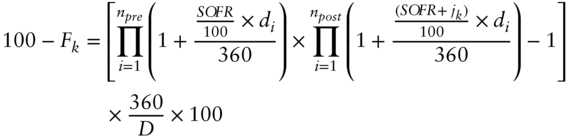
where
- npre and npost are the number of business days before and after k in the reference period of Fk.
- SOFR is the rate at the beginning of the reference period (assumed to be constant except on day k) and jk is the jump of SOFR following the FOMC policy announcement on day k.
Moreover, one can assess the impact of Fed policy on the spread between 1M and 3M contracts and adjust the hedge ratio between the two. To illustrate the problem, Figure 2.16 depicts two different positions of a FOMC meeting date in the 1M versus 3M SOFR future spread:
- If the meeting is right in the middle of the reference quarter of the 3M future and between the reference months of the 1M futures, distributing the hedge equally across the 1M futures – as in the standard 10 versus 3/3 hedge ratio – works well. The FOMC meeting schedule often comes relatively close to this ideal scenario, with the meetings in March, June, September, and December tending to be held at the 3rd Wednesday, i.e., at the start and end date of the reference quarters, while the meetings in the other months are often held around the turn of the month, i.e., near the start and end dates of the reference month.
- If, on the other hand, the meeting takes place at a distance from the middle, it affects the three contracts involved unevenly. The further the meeting date shifts to the right, the less it affects the 1M contracts relative to the 3M contract. Imagine the extreme scenario of the meeting taking place on May 30 rather than May 4. In this case, only one day of the reference month of the 1M futures would be affected, while there are still 15 affected days of the reference quarter of the 3M contract. Hence, in order to maintain the hedge against Fed policy shifts, the further the meeting date is to the right in Figure 2.16, the more of the later 1M future needs to be used relative to the 3M future, resulting in a deviation from the standard 10 versus 3/3 hedge ratio.17
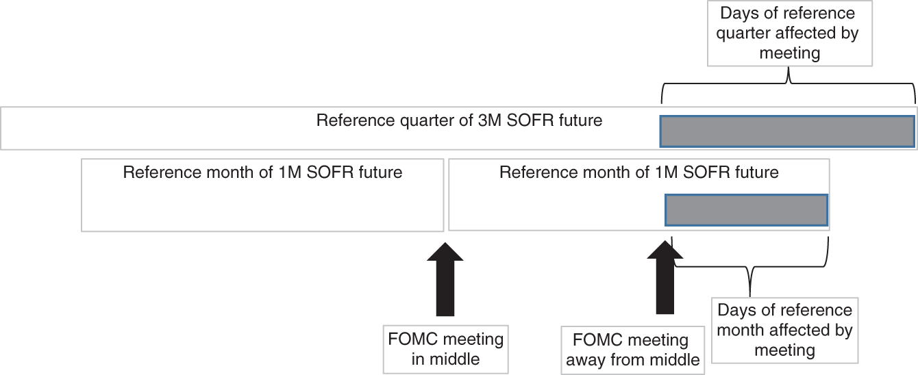
FIGURE 2.16 FOMC meeting dates relative to the reference periods of 1M and 3M SOFR futures
Source: Authors
A shift of the FOMC meeting date away from the middle to the right therefore results in a relative decrease of the sensitivity of 1M futures versus the sensitivity of 3M futures to the Fed policy and hence to a major source of yield volatility at the short end.
The sheet “3M versus 1M with FOMC hedge” illustrates how the hedge ratio for 3M versus 1M contracts could be adjusted to maintain neutrality versus the overall level of rates while also gaining neutrality versus Fed policy changes. Hence, in case the SOFR is only affected by Fed policy, i.e., follows a jump process,18 the 3M–1M future spread should be completely hedgeable via such a method.
This sheet calculates the hedge of the 3M Mar 2022 futures contract versus the two 1M contracts Apr 2022 and May 2022. The start and the end dates of the reference quarter coincide with the FOMC meeting dates (March 16 and June 15). During the reference quarter, one FOMC meeting takes place on May 4, 2022. As this is slightly away from the middle, one may ask how to adjust the standard hedge ratio (ten 3M versus three 1M futures each) to account for the (slightly) different exposure to a rate hike on that date.
First, the sensitivity of the 3M contract to changes of the level of SOFR (at the start of the reference quarter) and to the Fed rate hike on May 4 needs to be calculated. This can be done by assuming reasonable starting values in cells C2 and G2 and assessing the impact of a 1 bp bump in each (separately) (cell H8). The result is a sensitivity of −25.02 USD to +1 bp of the SOFR level and of −11.27 USD to +1 bp of the rate hike (cells H10 and H11).
Then, the sensitivity of the 1M contract affected by the Fed hike (May 2022) is calculated by dividing the days post-meeting by the total number of days in the reference month May. The result is a sensitivity of −36.29 USD to +1 bp of the rate hike (cell L2). In a first step, the 3M–1M future spread can be immunized against the Fed rate hike by taking the quotient of the two sensitivities, i.e., by selling 0.31 1M May 2022 contracts for every 3M Mar 2022 futures contract bought (cell K6). This approach works since the other 1M contract (April 2022) is not affected by the rate hike.
Hence, in a second step, the 1M Apr 2022 future can be used in order to obtain immunity against the rate level without influencing the hedge against the Fed rate hike already obtained in the first step. Selling 0.29 1M Apr 2022 contracts (cell K12) gives this immunity. Thus, the hedge consists in selling 3.1 1M May 2022 and 2.9 1M Apr 2022 contracts for every ten 3M Mar 2022 futures bought. The slight deviation of the meeting date from the middle therefore results in a slight deviation from the standard hedge ratio. The calculation of the hedge in two steps can be expressed in two simple formulae:

where
- nApril and nMay is the (short) position in 1M April and May SOFR futures for each one (long) 3M Mar 2022 future.
- dpost is the number of calendar days in the reference month of the 1M May future after the FOMC announcement.
- dtotal is the total number of calendar days in the reference month of the 1M May future (31).
- sj is the price sensitivity of the 3M Mar 2022 future to a 1 bp increase in the jump of SOFR following the FOMC announcement.
- sl is the price sensitivity of the 3M Mar 2022 future to a 1 bp increase of the SOFR at the beginning of the reference quarter.
When the FOMC meeting date is further off the middle (Figure 2.16), the adjustment relative to the standard hedge ratio becomes larger. For the example of the 3M Sep 2018 contract, when the meeting took place on Nov 8, 2018,19 the hedge ratio was 2.24 1M Oct 2018 and 3.79 1M Nov 2018 futures per ten 3M Sep 2018 contracts.
This mechanism implies that depending on the FOMC meeting schedule and policy expectations, 3M SOFR futures can be more affected by changing expectations about the Fed policy than the standard combination of 1M SOFR futures. That is another way of expressing the result from above, that a higher number than six for the sum of the 1M contracts is required in order to adjust for the lower sensitivity. For example, for ten 3M Sep 2018 contracts, a total of 6.03 1M contracts were needed to obtain immunity. This also explains the observation, that sometimes – i.e., depending on the FOMC meeting situation – 1M SOFR contracts appear to move less than 3M futures or the term rate.20 The relatively small moves of 1M futures may seem puzzling if one only considers parallel shifts of the SOFR curve; they become clearer when one also considers their sometimes-lower exposure to Fed policy, a major source of rate volatility at the short end. Analysts are well advised to keep this in mind, in particular when using 1M futures to hedge or replicate other instruments, such as 3M contracts or the term rate.
PRICING AND HEDGING WITH SOFR FUTURES: GENERAL CONSIDERATIONS
Using the adjustments just outlined, one can easily transfer the pricing and hedging techniques from ED to SOFR contracts. For example, one could use a strip of SOFR futures to replicate and hedge a term SOFR. However, this method does not work well when the term and the end date of the futures strip are different – when an FOMC meeting falls between the two. In this case, an allowance for the curve between the two dates (e.g., the jump at the FOMC meeting date) is desirable.
Therefore, traders nowadays usually construct curves from futures markets and apply these to solve pricing and hedging questions. For example, focusing on the effect of Fed policy on the yield curve only, one could calibrate a jump process to the prices observed in the futures market and obtain the rates at any forward date from this process. Of course, after taking into account the required adjustments for the front month contract, SOFR futures also can be used as input into these common curve construction techniques.
The first key decision is the choice of the functional form for the curve:
- The future strip used for the simple term rate hedge just mentioned corresponds to the assumption of the SOFR curve following a jump process, with the jumps occurring at the contract dates of the SOFR futures (in case of 1M SOFR contracts, the turns of the months). Between the contract dates, the same single forward SOFR value implied by the future price is used. Hence, if the forward point in time required (e.g., for hedging a term rate of a swap) does not fall on a contract date, the assumption of a constant curve between the two can lead to mismatches. There are a number of ways to react to this problem:
- The first possible approach is to use some sort of interpolation between the contract dates. Starting with linear interpolation, more sophistication can be reached by using exponential or cubic splines. This tends to produce good results from the middle part of the yield curve onward, where the impact of specific Fed policy decisions on the curve becomes less decisive and the FOMC meeting dates are unknown.
- The second possible approach is to stick with the jump process, but to use the FOMC meeting dates rather than the contract dates as the points in time when the jumps occur. Furthermore, specific points in time, such as the year-end, when spikes in SOFR are expected can be added as jump dates. This is useful for the short end of the curve, on which the Fed policy has an overwhelming effect and the FOMC meeting dates are known. Figure 2.17 illustrates the possibilities mentioned so far, for reasons of visibility for 1M SOFR futures only.
- In case the same jump process is used as the CME applies in its Term rate calculation (see Chapter 3), the construction of the SOFR curve simultaneously allows calculation of the Term rate; likewise, the same method used for hedging swaps with SOFR futures can be applied to hedge the CME Term rate with SOFR futures. The advantage of this approach is that it kills two birds with one stone. The disadvantage is that it subjects the SOFR curve and swap hedge to the same problems and criticisms of the Term rate mentioned in Chapter 3 and cannot be used for option pricing.
- Combining both approaches, one can add jumps to a cubic spline, for example. In the framework described in Chapter 11 of Huggins and Schaller 2013, the contract dates of the 3M futures could be used as anchor points for the cubic spline and the FOMC meeting dates as external variables. This combination has the advantage of producing a single yield curve from the short to the long end, which takes the effect of Fed policy on the short end into account but also minimizes frictions.
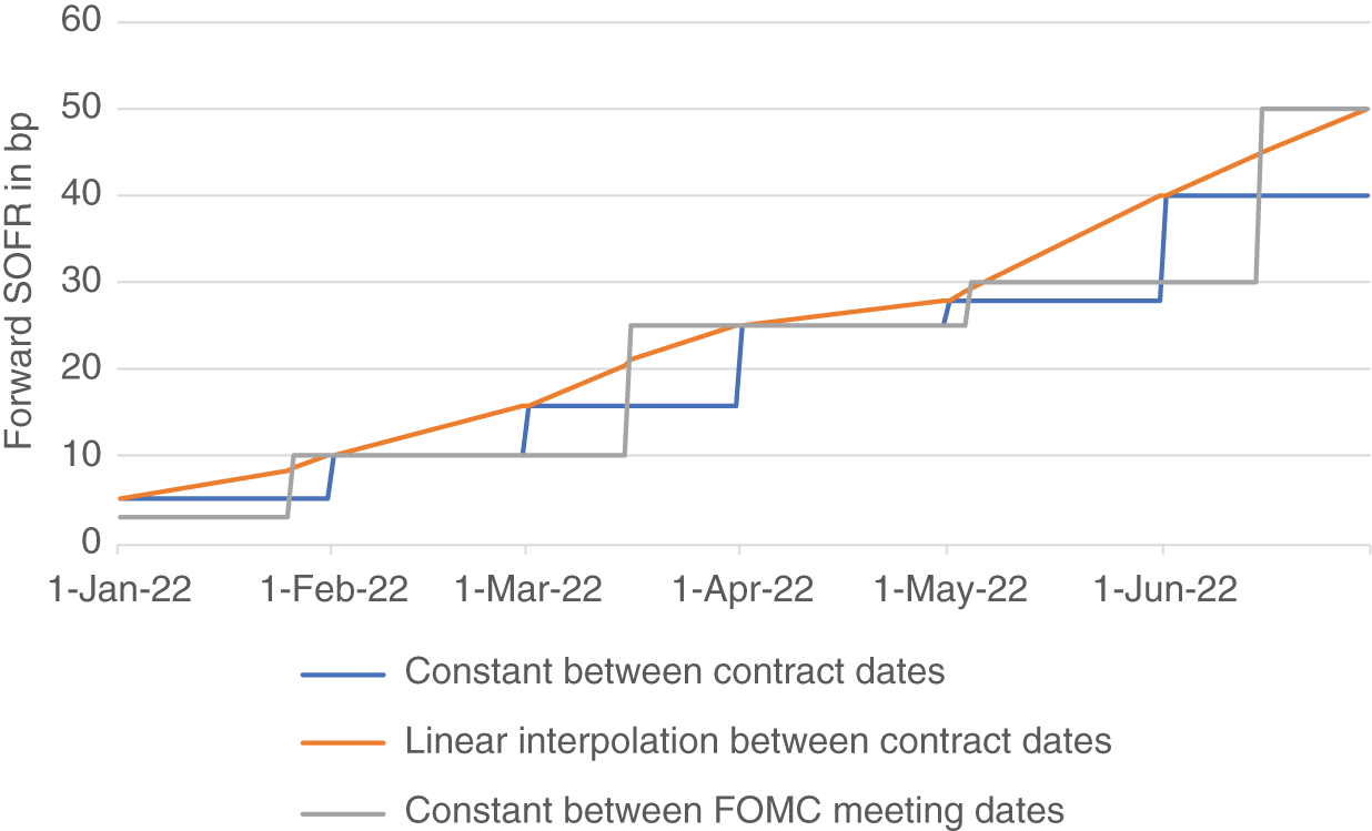
FIGURE 2.17 Different functional forms for the forward SOFR curve
Source: Authors
- Alternatively, one could combine the jump process with a stochastic process in order to account for the yield volatility not coming from Fed policy. A good candidate for a mixed jump-diffusion process could be a one-factor Hull-White model with jumps at the FOMC meeting dates. That is, when a jump occurs, both SOFR and the mean around which it reverts jump by similar amounts. Due to the diffusion, this process produces usually more reasonable option prices and can therefore be used to model both futures and the options on them, avoiding discrepancies.
Once the fundamental questions about the process are decided, the set of futures used for calibrating the process must be determined. Also this step offers several possibilities and requires therefore discretion and experience:
- When the number of futures contracts is less than the number of parameters used to describe the short rate process, the problem is said to be underdetermined. When the number of futures contracts is greater than the number of parameters, we say the problem is overdetermined. Calibrating a jump process with the FOMC meeting dates as unknown variables to all 1M and 3M SOFR futures as known variables, for example, is usually significantly overdetermined.
- One can either construct the SOFR curve from SOFR futures, and then separately the LIBOR curve (from ED contracts) and then separately the FF curve (from FF contracts), or all simultaneously. In the first case, the basis between the curves is given by the external spread between the separately constructed curves; in the latter case, it is an internal parameter of the curves constructed from all futures simultaneously. The simultaneous construction can be thought of as decomposing the information contained in the whole STIR (short-term interest rate) future universe into information about market expectation about Fed policy (influencing all STIR contracts) and information about the secured–unsecured basis. When considering only SOFR-related instruments (e.g., a SOFR term rate hedge with SOFR futures), the separate construction offers the advantage of excluding influences from unsecured rates. The combined approach is useful whenever the basis between secured and unsecured rates is involved in the pricing (e.g., when the switch of an asset swap of a government bond from LIBOR to SOFR as floating leg should be hedged with SR1:FF spread contracts). (See Chapter 4.)
Pricing and hedging is not a mechanical procedure but requires the careful assessment of the different possibilities to achieve the specific hedging goals, which can be different from hedger to hedger. The selection of the process and its implementation introduces a significant degree of discretion: There is not the hedge, but several different possible hedges, which work better or worse for a given task. This also introduces the opportunity for analysts and traders to outperform competitors by improved hedging.
Given the number of possibilities already for selecting the functional form of the curve and the number of different hedging goals, a complete discussion is outside the scope of this book. But it does provide a few examples, which the reader may find useful as a starting point for constructing his own pricing and hedging tools.
EFFECT OF PROCESS SELECTION ON THE PRICING OF SOFR FUTURES
To assess the effect of the choice of the functional form and the parameters of the process used for pricing SOFR futures, one can start with a jump-diffusion process as a general framework, which covers both a pure jump process (by setting the volatility parameter to 0) and a pure diffusion process (by setting the probability for a jump to 0) as special cases. Moreover, one can add drift terms – for example, for mean reversion and momentum. The links between all these elements need to be considered (e.g., the impact of jumps on the drift and diffusion parameters). In the Hull-White model just mentioned, the mean could be shifted by the amount of the jump, for instance. Alternatively, one could consider jumps as being part of the mean reversion or diffusion.
Given our goal of demonstrating the effect of process selection on the pricing, and given the limitations of Excel spreadsheets, we use a simple Vasicek process – that is, one drift term for the mean reversion and one diffusion term – and add jumps at specific dates. We do not consider the links between these elements (e.g., the impact of jumps on the mean reversion parameters). Hence, this example should be considered a “heuristic framework.” In the absence of an analytic solution for the combination of all the elements, numerical simulation needs to be applied. An example for such a simulation is encoded in the Excel sheet “SOFR future price simulation” accompanying this chapter. Please note that, like all sheets presented here, its goal is to illustrate concepts for educational purposes, and they are not fit for application in a professional context. Specifically, again due to the limitations of Excel sheets, we use only 200 simulations (in the columns), which is significantly too few; when applied with money at stake, many more simulations are required. (One million simulations would be more typical.)
Let us assume that on Jan 1, 2022, one wants to price the Mar 2022 SR3 contract (with a reference quarter from Mar 16 to Jun 15). To simplify the situation by reducing the parameters, we also assume that there is zero probability for a change in Fed policy at the FOMC meeting on Jan 26 and for any unscheduled FOMC meetings. This leaves two FOMC meetings to consider, on Mar 16 (i.e., right at the start of the reference quarter) and on May 4, for which we assume that the policy rate either increases by 25 bp or remains the same, with the probability for a 25 bp hike being set in cells E6 and E10. Cells E1 to E4 define the parameters for a Vasicek process, assuming that the start value for SOFR on Jan 1, 2022, is 5 bp. Based on this input, beginning in row 15, the SOFR evolution is modeled, assuming the standard deviation is the same for each calendar day.21 For each of the simulated paths, the compounded SOFR during the reference quarter is calculated (row 135) and the average over all simulations is shown in cell H1.
Let us further assume that one decides to price the future according to the average of the simulated settlement prices (cell H2). This assumption ignores other influences on the future price. However, given the results of Chapter 6 and the short horizon of the simulation, this simplification could be acceptable for our current goal to obtain a first impression of the impact of different processes and their parameters on the future pricing.
Table 2.2 depicts the simulated future price, divided into the three main cases of a pure jump process,22 a pure diffusion (and drift) process and a combined jump-diffusion (and drift) process, each with subcases for different parameters:
- As expected, the simulated settlement price depends heavily on the assumed probabilities for Fed rate hikes. This is in line with the common-sense perception that Fed policy has a major impact on the short end of the curve and hence the pricing of STIR contracts.
- Since the Vasicek process used assumes a symmetric distribution of the diffusion, the standard variation parameter has little impact on the simulated settlement prices; higher variance of the diffusion process – reflecting the volatility of SOFR not coming from Fed policy – does lead to some smoothing-out; however, the impact of jumps on future prices is more visible in an environment of lower diffusion.
- Also in line with the expectation, both the mean and speed of mean reversion parameter have a significant impact on the simulation result. One should note the correlation of these parameters with the jump probabilities: When rates are low as at the beginning of 2022, there is both a higher probability for Fed hikes than for cuts and a pull toward the mean from the drift coefficient in the Vasicek process. When building a jump-diffusion model, this link – which is not treated in the Excel sheet – should be taken into consideration.
The impact of the drift term is shown in Table 2.3 via a few combinations of the values for the mean and for the speed of mean reversion, represented in a two-dimensional matrix, and assuming 0.05% as start value and 2% as annualized standard deviation.23 It can be seen that, even for the short horizon considered in this simulation, these two parameters have a major effect on the simulation results.
Therefore, even this simple simulation reveals the high dependency of the pricing on the choice of the process and its parameters. Extensive research into this topic is therefore a good investment. Under the impression of Table 2.3, in case of a drift term being part of the process, investigating the mean reversion of SOFR can be considered as a vital part of this exercise. Since the history of SOFR is limited, one can use other short-term rates as proxies in order to assess the mean reversion characteristics over several rate cycles. When using a Vasicek model, it makes sense to estimate the parameters from historical time series by calibrating an Ornstein-Uhlenbeck process. Expanding the SOFR series with the overnight GC primary dealer survey rate back to 1998, we obtain an estimated mean of 1.18% and an estimated speed of mean reversion of 0.006. Figure 2.18 depicts the input and output of this mean reversion process. As the time series contains sharp spikes,24 the question is whether to include these spikes when calculating the parameters given the recent establishment of the Fed's standing repo facility. (See Chapter 1.) If the spikes are excluded, the speed of mean reversion parameter decreases. This is one example for the discretion involved in every detail of the modeling process. When including the spikes and sticking to these parameters for a pure diffusion process, the average simulated settlement price of the Mar 2022 SR3 contract would be 99.4392.
TABLE 2.2 Simulated average settlement price of the Mar 2022 SR3 future
Source: Authors
| MAIN CASE 1: ONLY JUMP(S): Probability of +25 bp jump at | Settlement price | |
|---|---|---|
| Meeting Mar 16 | Meeting May 4 | |
| 0% | 0% | 99.9500 |
| 0% | 50% | 99.9010 |
| 0% | 100% | 99.8373 |
| 50% | 0% | 99.8251 |
| 50% | 50% | 99.7747 |
| 50% | 100% | 99.7198 |
| 100% | 0% | 99.7026 |
| 100% | 50% | 99.6468 |
| 100% | 100% | 99.5899 |
| MAIN CASE 2: ONLY DIFFUSION AND DRIFT | |||
|---|---|---|---|
| Standard Deviation (ann) | Mean | Speed of mean reversion | |
| 1% | 1.50% | 0 | 99.9212 |
| 2% | 1.50% | 0 | 99.8912 |
| 5% | 1.50% | 0 | 99.9099 |
| 2% | 1.50% | 0.002 | 99.7686 |
| 5% | 1.50% | 0.002 | 99.7130 |
| 2% | 3.00% | 0.002 | 99.5139 |
| 5% | 3.00% | 0.002 | 99.4326 |
| MAIN CASE 3: JUMP-DIFFUSION (AND DRIFT) | |||||
|---|---|---|---|---|---|
| Standard Deviation (ann) | Mean | Speed of mean reversion | Meeting Mar 16 | Meeting May 4 | |
| 2% | 1.50% | 0 | 50% | 50% | 99.7469 |
| 2% | 1.50% | 0 | 100% | 100% | 99.5650 |
| 2% | 1.50% | 0.002 | 50% | 50% | 99.5466 |
| 2% | 1.50% | 0.002 | 100% | 100% | 99.3825 |
| 5% | 1.50% | 0.002 | 50% | 50% | 99.4828 |
| 5% | 1.50% | 0.002 | 100% | 100% | 99.4211 |
| 2% | 3.00% | 0.002 | 50% | 50% | 99.3066 |
| 2% | 3.00% | 0.002 | 100% | 100% | 99.1670 |
TABLE 2.3 Simulated average settlement price of the Mar 2022 SR3 future using a pure Vasicek process
Source: Authors
| Mean | |||||
|---|---|---|---|---|---|
| 0% | 1,5% | 3% | 5% | ||
| Speed of mean reversion | 0.000 | 99.9500 | 99.9500 | 99.9500 | 99.9500 |
| 0.001 | 99.9563 | 99.8603 | 99.7101 | 99.5842 | |
| 0.002 | 99.9699 | 99.7686 | 99.5139 | 99.1756 | |
| 0.005 | 99.9840 | 99.4316 | 98.9558 | 98.2250 | |
| 0.010 | 99.9869 | 99.1365 | 98.2527 | 97.1213 | |
The reasoning above is an illustration for the first step toward a pricing model for SOFR futures, with the remaining steps depending on the individual market assessment, specifically the weight given to Fed policy, and goals of the reader. But even at the end of the long journey to a pricing model, it is useful to remember alternative process and parameter choices. Coming back to the detail just mentioned, one could calculate the parameters of the mean reversion process without spikes in the input time series, obtain a speed of mean reversion of 0.002 and with this as input parameter into the simulation an average settlement price of 99.7615. Hence, even the question of whether to include a few spikes or not in the historical time series, which might seem trivial at first glance, can have a material impact on the model prices. Obviously, this is even more the case for the fundamental decision about the relative weight given to jumps versus drift and diffusion, which is related to the fundamental worldview about the relative importance of Fed policy for STIR contract pricing. Even if a trader takes the extreme view that only Fed policy matters and hence uses a pure jump process, he is well advised to also look at a combined jump-diffusion process in order to stress-test his SOFR future pricing under the scenario of SOFR being influenced by factors not related to Fed policy as well.
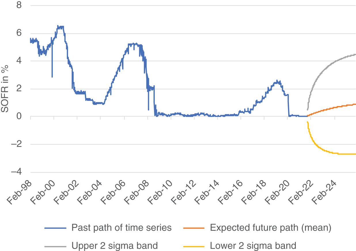
FIGURE 2.18 SOFR (proxy) as modeled by an Ornstein-Uhlenbeck process
Source: Authors, based on data from CME
Chapter 5 will expand this simulation and the Excel workbook to assess the impact of process and parameter selection on the pricing of options on SOFR futures. In line with the anticipation, we will find that the standard deviation parameter matters more for pricing options on futures than for pricing futures themselves. Hence, even if a trader decides to use a pure jump model for pricing futures, maybe arguing that the drift from mean reversion is sufficiently incorporated in the jumps, the trader will face the issue of the neglected diffusion term when turning to pricing options on futures. To use one model for consistent pricing of both SOFR futures and the options on them, therefore, the trader might want to consider including a diffusion term right from the beginning.
EXAMPLE FOR HEDGING A SOFR TERM RATE WITH SOFR FUTURES VIA A JUMP PROCESS
After the functional form of the curve and the set of futures used for calibration have been determined, the process can then be used to calculate the hedge ratios that immunize a portfolio. Using the example of the jump process, one can calculate the effect of a change in its parameters – i.e., the rate at the beginning and each jump, on every SOFR future on one hand and on a term rate on the other hand – and then construct a set of SOFR futures with the same exposure to all changes in the parameters as the term rate. This general approach, illustrated in Figure 2.19, can be modified to hedge a term rate (Chapter 3) and (asset and basis) swaps (Chapter 4) with SOFR futures.
Imagine the task is to hedge a 6M term rate starting on Jan 1, 2022, with a portfolio of SOFR futures, for example, because a dealer knows on Oct 1, 2021, that he is going to have exposure to a 6M SOFR term rate in 3M time. As mentioned above, the first key decision to take concerns the process used; for this example, we apply a simple jump process, assuming that FOMC meetings are the only source of interest rate volatility. Our reason for this choice is not that we consider this to be the only or the best alternative; actually, we will criticise this process in Chapter 3. We have selected it nevertheless because it fits both to the hedge against FOMC meetings described above and to CME's Term rate calculation described in Chapter 3. Note, however, that it is not identical to CME's Term rate; for instance, the jump process applied here cuts off after 6M, so that its 6M term rate does not depend on events beyond the 6M horizon, as does CME's Term rate. Hence, this example should be considered as illustration of one relatively easy (not necessarily the best) way to hedge a (not CME's) SOFR term rate; it shows a hedge of a term rate, not the hedge of the term rate. A precise hedge of CME's Term rate is significantly more complex and will be treated in Chapter 8.
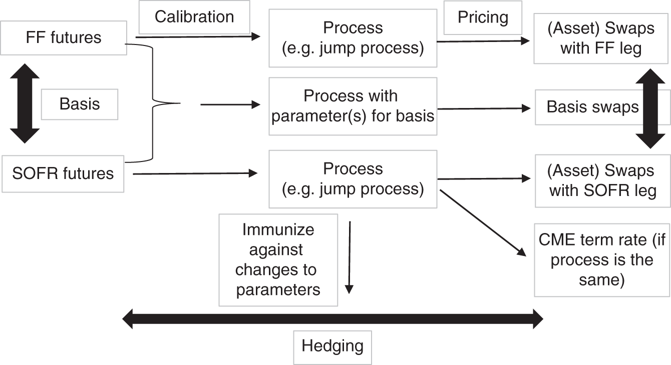
FIGURE 2.19 Futures as a hedge via calibrating a process
Source: Authors
For the sake of this example, we select the jump process
where
- t0 is the start of the term.
- M is the set of all FOMC policy announcement dates between t0 and t.
- jk is the jump of SOFR following the FOMC policy announcement on day k.
In a first step, we calculate the sensitivities of both the 6M term rate and the SOFR futures to changes of the parameters of this jump process, i.e., the level (SOFRt0) and the jumps (jk). This can be considered as an expansion of the method described as hedge against the impact of FOMC meetings above. It is encoded in the Excel sheet “Term rate hedge example” accompanying this chapter.
For this particular example, there are four FOMC meetings during the 6M term. The sensitivity table (cells G15 to N19) can be filled out as described above:
- Bumping the start value and the jumps (separately) gives the sensitivity of the term rate (cell G7) and the 3M Mar 2022 SOFR future (cell G10). The reference quarter of the latter is highlighted in bold in the compounding column D. Alternatively, the formula above could be applied.
- The sensitivity of the 1M contracts to FOMC meetings in their reference month is given by the formula above and encoded in cells L2 to L5. To the other FOMC meetings, the sensitivity is simply 0 or 1, depending on whether it is after or before the reference month.
At this stage, we face the overdetermination problem mentioned: Even though we use only futures whose reference period is fully inside the 6M term (not including the Dec 2021 and Jun 2022 SR3 contracts), there are seven of those, i.e., seven potential hedging instruments, for only five parameters to be hedged. Like for the selection of the process, discretion and experience is required to select the best set of hedging instruments. It seems that including the 3M future (Mar 2022) and excluding the 1M futures fully in its reference quarter (Apr and May 2022) is both reasonable and produces reasonable numbers. Of course, one can and should try different combinations and compare the results; if the results are too different, one could even think of going a step back and consider another process. While our experience is limited, we found that this method can sometimes lead to unrealistic results – in particular, when only 1M futures are used.25
Another point to consider when determining the futures used for the hedge is the number of days post the FOMC meeting (npost). When it is small relative to the total number of days in a reference period, the number of futures required to immunize against this jump becomes large – and hence this “overhedge” needs to be corrected by a large number of offsetting positions in other contracts. This is one reason behind sometimes unrealistic outcomes. If such a situation occurs, it is advisable to exclude these contracts, perhaps by replacing them with 3M futures.26
With this in mind, we may decide to hedge the 6M term rate with Jan, Feb, Mar, and Jun SR1 contracts and the Mar SR3 future. This is now a well-defined hedging problem (five instruments for five parameters), which can be solved by usual matrix algebra, as encoded in the sheet below the sensitivity table. The resulting hedge portfolio of SOFR contracts shown in cells M31 to M35 consists of 0.17 Jan SR1, 0.14 Feb SR1, 0.19 Mar SR1, 0.17 Jun SR1, and 0.33 Mar SR3 futures. Note that these numbers are in bp terms, i.e., represent the hedge against a 1 bp move in the 6M term rate. To obtain the number of futures, they would need to be divided by the basis point values of the futures contracts (41.67 for 1M, 25 for 3M) and multiplied by the basis point value of the exposure to the 6M term rate.
NOTES
- 1 The calculations of settlement prices and spreads for these contracts are illustrated in the Excel sheet “3M versus 1M” accompanying this chapter.
- 2 The differences will be discussed in Chapter 4.
- 3 A few data points have been excluded due to illiquidity.
- 4 Chapter 5 will link this observation to Asian options.
- 5 Burghardt et al. (1991) can be considered as starting point for many for these analyses.
- 6 Chapter 5 will provide more details on this.
- 7 The details of the data aggregation applied are explained in Chapter 5.
- 8 An interesting question is whether market expectations for secured rates (as implied in SOFR futures) are a better predictor for actual Fed policy than those for unsecured rates (as implied in ED futures).
- 9 As in this example the term is less than one year, N = 0 and the annualization formula can be simplified.
- 10 Also this figure and the numbers for the Dec 19 roll example apply the data aggregation outlined in Chapter 5.
- 11 Again, a slightly different holiday schedule applies.
- 12 This is a hypothetical assumption not in line with the FOMC meeting calendar in order to illustrate the point.
- 13 CME, April 2018.
- 14 Still, especially in low interest rate environments, it may be useful to keep the slight deviation of the CME convention from the actual (3+3)-to-10 spread in mind.
- 15 See Chapter 3.
- 16 One could argue that it is not certain that a change of 25 bp in the Fed Funds rate corresponds to a change of 25 bp in SOFR. However, as long as we are only dealing with SOFR futures, any difference is likely to net out: since 1M and 3M SOFR futures would need to be adjusted with the same factor for the move in SOFR/move in FF, it would cancel out in the hedge ratio. But when looking at spreads between SOFR and FF futures, this secured–unsecured basis will become important and will be discussed in detail in Chapter 4.
- 17 If the meeting takes place after the reference month, this hedge is not possible at all any longer; this corresponds to the example of a 50 bp hike on Dec 1 from above.
- 18 This is the assumption behind CME's Term rate discussed in Chapter 3.
- 19 There was also a meeting on Sep 26, which needed to be included in the calculation.
- 20 Due to illiquidity, it is not yet possible to compare the relative pricing of options on 3M and 1M SOFR futures in that light.
- 21 The user can change the assumption to business days by replacing the input from column C into the simulation with the annualized standard deviation (cell E2) divided by the square root of the number of business days in the year 2022.
- 22 Due to the simulation, the standard deviation (cell E2) cannot be set to 0; using a very small value like 0.00001 works.
- 23 Due to the low number of simulations, we have taken the averages of several simulations. For a speed of mean reversion of 0, we have used the theoretical value.
- 24 Even though we use weekly intervals in order to exclude daily fluctuations.
- 25 In the examples we have considered, including the 3M contract has solved these problematic instances. But we cannot rule out that there are cases in which this method does not work.
- 26 If the first 1M contract (Jan 2022) was problematical, the replacement could be the Dec 2021 SR3 future, which would need to be adjusted for the days in its reference quarter before the term rate by the method described above.