CHAPTER 5
Risk Matrices, Lie Factors, Misconceptions, and Other Obstacles to Measuring Risk
We are ultimately trying to move cybersecurity in the direction of more quantitative risk assessment methods. The previous chapters showed that there are several methods that are both practical (the authors have used these methods in actual cybersecurity environments) and have evidence of measurably improving risk assessments. We offered an extremely simple method based on a one‐for‐one substitution of the components of a risk matrix. Anyone who has the technical skills to work in cybersecurity certainly has the skills to implement that solution. Once an analyst becomes familiar with the basics, he or she can build on the foundation we've provided with our methods in later chapters.
But regardless of the evidence shown so far, we expect to see resistance to many of the concepts shown. There will be sacred cows, red herrings, black swans, and a few other zoologically themed metaphors related to arguments against the use of quantitative methods. In this chapter we will address each of these issues. We have to warn you in advance: This chapter is long, and it will often feel like we are belaboring a point beyond what it deserves. But we need to systematically address each of these arguments and thoroughly make our case in a manner as airtight as the evidence allows.
Scanning the Landscape: A Survey of Cybersecurity Professionals
In preparation for making this comprehensive case, we wanted to understand something about the backgrounds and opinions that the cybersecurity industry had about many of the points we are making. We wanted to know the level of acceptance of current methods and perceptions about quantitative methods. So we asked 171 cybersecurity specialists from a variety of backgrounds and industries to answer some questions about statistics and the use of quantitative methods in cybersecurity. Survey participants were recruited from multiple information security–related groups including the Society for Information Risk Assessment (SIRA), ISACA, and three of the largest discussion groups on LinkedIn. There were a total of 63 questions covering topics such as personal background, their organizations, and breaches experienced. The survey also included questions related to the use of quantitative methods in cybersecurity and a quiz containing basic statistics‐literacy questions.
Part of the survey contained a set of 18 questions we referred to as Attitudes Toward Quantitative Methods (ATQM). These helped us assess the opinions of cybersecurity experts as being more supportive of the use of quantitative methods or more skeptical. Within the ATQM, we had two subsets. Some of the questions (seven, to be exact) had responses that were clearly more “anti‐quantitative,” such as, “Information security is too complex to model with quantitative methods.” These questions made much sharper distinctions between supporters and opponents of quantitative methods. Other questions were about attitudes that were not directly anti‐quantitative but indicated an acceptance of the value of nonquantitative methods—for example, “Ordinal scales help develop consensus for action.” Table 5.1 shows a few examples from each group of ATQM questions.
TABLE 5.1 Selected Examples of Survey Questions About Attitudes toward Quantitative Methods
| Statement from Survey | Percent Agreeing (Positive Responses/Number Responding) |
|---|---|
| Ordinal scales must be used because probabilistic methods are not possible in cybersecurity. | 18% (28/154) |
| Probabilistic methods are impractical because probabilities need exact data to be computed and we don't have exact data. | 23% (37/158) |
| Quantitative methods don't apply in situations where there are human agents who act unpredictably. | 12% (19/158) |
| Commonly used ordinal scales help us develop consensus for action. | 64% (99/154) |
We found it encouraging that most who work in cybersecurity (86%) are generally accepting of more quantitative methods based on probabilistic models; that is, they answered more of the “opinions about quantitative methods” in a way that supported quantitative methods. For example, most (75%) agreed with the statement “Cybersecurity should eventually adopt a more sophisticated probabilistic approach based on actuarial methods where it has not already done so.”
However, only 32% were always supportive of quantitative methods (i.e., 68% disagreed with some of the statements preferring quantitative methods to softer methods). Even those who support more quantitative methods see value in the continued use of softer methods. For example, 64% agreed with the statement “Commonly used ordinal scales help us develop consensus for action,” and 61% stated that they use risk matrices. There is even a small but significant minority (8.3%) who tended to be more anti‐quantitative than pro‐quantitative. This is a concern because vocal minorities can at least slow an adoption of quantitative methods (the authors have seen some cases of this). And even the majority who are generally accepting of quantitative may be slow to adopt better methods only because it seems a bit too challenging to change or because current methods are perceived as adequate even if flawed.
Of course, any survey that relies on voluntary responses could have a selection bias, but it would not be clear whether such a selection bias would be more “pro‐” or “anti‐”quantitative. Still, the level of acceptance of quantitative methods was on the high end of what we expected. Some readers may already question the methods, sample size, and so on, but the statistical significance—and the academic research credentials of the Hubbard Decision Research staff who analyzed the results—will be discussed shortly.
If you personally have reservations about moving cybersecurity risk assessment in the direction of quantitative methods, see if your specific reservation is discussed in this chapter and consider the counterargument. If you are a fan of quantitative methods and we are preaching to the choir, then familiarize yourself with this chapter so that you might be better able to respond to these objections when you hear them.
At first glance, the arguments against the use of quantitative methods seem to be many and varied, but we make the case that these points all boil down to a few basic types of fallacies. We will start by investigating a collection of methods that are currently the most popular in cybersecurity risk assessments: the ordinal scales on a risk matrix. Once we can shine a light on the problems with these techniques and objections, we hope we can move past this to implement mathematically sound risk assessment in a field that needs it badly.
What Color Is Your Risk? The Ubiquitous—and Risky—Risk Matrix
Any cybersecurity expert will recognize and likely embrace the common risk matrix, which is based on ordinal scales. In fact, based on our experience, most executives will laud the risk matrix as “best practice.” As mentioned in Chapter 1, these scales represent both likelihood and impact, not in probabilistic or monetary terms but in ordinal scales. The scales might be represented with labels such as low, medium, or high, or they might be represented as numbers on a scale of, say, 1 to 5. For example, a likelihood and impact might be represented as a 3 and a 4, respectively, and the resulting risk might be categorized as “medium.” These scales are then usually plotted onto a two‐dimensional matrix where the regions of the matrix are further categorized into “low” to “high” risk or perhaps given colors (“green” is low risk, while “red” is high). In some cases, ordinal scales are used without a risk matrix. Perhaps several ordinal scales are added together in an overall risk score, as is the case with OWASP's risk rating methodology.1 (Note: OWASP, like many frameworks, has great controls recommendations, but a controls checklist does not equate to a risk management methodology.) The scales focus on attributes that might indicate risk (such as “ease of discovery” or “regulatory impact”). Then these scores are categorized still further into high, medium, and low risk just like a risk matrix.
As mentioned in Chapter 2, ordinal scales are not in themselves necessarily a violation of measurement theory or statistics. They do have legitimate applications. But are they substitutions for ratio scales of probability and impact? Meaning, are they some form of vague stand‐in for probabilities, as have already been used in insurance, decision science, statistics, and many other areas? Should substituting ordinal scales such as “high” or “medium” for more quantitative measures strike us as just as odd as an engineer saying the mass of a component on an airplane is “medium,” or an accountant reporting that revenue was “high” or a “4” on a scale of 5?
These are important questions because risk matrices using ordinal scales to represent likelihood and impact are common in cybersecurity. In the survey we found that 61% of organizations use some form of the risk matrix, and 79% use ordinal scales to assess and communicate risks. Even partial use of some of the statistical methods, for which we provided so much evidence of their effectiveness in Chapter 4, are much less common. For example, only 13% of respondents say they use Monte Carlo simulations, and 14% say they use some form of Bayesian methods (although both of these are actually much more common responses than the authors expected).
Some form of these ordinal scales are promoted by just about every standards organization, consulting group, and security technology vendor that covers cybersecurity. Dozens if not hundreds of firms help organizations implement methods or software tools that utilize some form of scores and risk matrices. The International Organization for Standardization (ISO) standard 31010 states that the risk map (what Table A.1 of the standard refers to as a “consequence/probability matrix”) is “strongly applicable” for risk identification.2
Clearly, these methods are deeply intertwined in the ecosystem of cybersecurity. However, as widely used as these scales are in cybersecurity, there is not a single study indicating that the use of such methods actually helps reduce risk. Nor is there even a study that merely shows that individual judgment is improved in any way over expert intuition alone. Granted, there are a lot of advocates of such methods. But advocates, no matter how vocal, should be considered cautiously given the research about the possibility of analysis placebo effects mentioned in Chapter 4.
On the other hand, several studies show that the types of scales used in these risk matrices can make the judgment of an expert worse by introducing sources of error that did not exist in the experts’ intuition alone. In fact, we believe that these methods are like throwing rocket fuel on a fire. We have enough uncertainty in battling hard‐to‐detect threats; why make it worse by abstracting away data through questionable scales?
In the book The Failure of Risk Management, Hubbard spends an entire chapter reviewing the research about the problems with scores. Subsequent editions of his book How to Measure Anything added more sources as new studies finding problems with these scales were identified. To help make this issue clear we will use the same approach used in Chapter 4. That is, we will look at research regarding three key components of the issue:
- The Psychology of Scales: The psychological research behind how we use verbal scales such as “unlikely” to “likely” to evaluate the likelihood of an event, and how arbitrary features of verbal or numeric (e.g., 1–5) ordinal scales affect our choices.
- Math and the Risk Matrix: The mathematical problems associated with attempting to do math with ordinal scales or presenting them on a risk matrix.
- How These Issues Combine: Each of the two issues above is bad enough, but we will show some research that shows what happens when we consider these effects together.
The Psychology of Scales and the Illusion of Communication
Ordinal scales are widely used because of their simplicity, but the psychology of how they are actually used is not quite so simple. The human expert using a scale has to be thought of as a kind of instrument. The instrument can have surprising behaviors and the conditions that elicit these behaviors should be investigated. As we did in earlier component analysis, we resort to research in other fields when research in cybersecurity specifically is lacking.
One component of risk scales that has been researched is how we use words to describe likelihoods. Researchers such as the psychologist David Budescu published findings about how differently people will interpret terms that are meant to convey likelihood such as “unlikely” or “extremely likely.” This ambiguity obviously would allow for at least some different interpretations, but Budescu wondered how varied those interpretations might be. He had subjects in his experiment read phrases from the Intergovernmental Policy on Climate Change (IPCC) report. Budescu would give his survey subjects a phrase from the IPCC report, which included one of seven probability categories (e.g., “It is very likely that hot extremes, heat waves, and heavy precipitation events will continue to become more frequent”). Budescu found that individuals varied greatly by how much they interpreted the probability implied by the phrase. For example, Budescu finds that “Very likely” could mean anything from 43% to 99%, and “Unlikely” could mean as low as 8% or as high as 66% depending on whom you ask.3
The subjects in Budescu's study were 223 students and faculty of the University of Illinois, not professionals charged with interpreting that kind of research. So, we might wonder if these findings would not apply to an audience that is more skilled in the topic areas. Fortunately, there is also supporting research in the field of intelligence analysis—a field cybersecurity analysts might appreciate as being more relevant to their profession.
One of these supporting studies was conducted by Sherman Kent, a Yale history professor and a pioneering CIA analyst who is often referred to as “the father of intelligence analysis.” Kent asked 23 NATO officers to evaluate similar probability statements.4 Similar to what Budescu found for “Very likely,” CIA researchers found that the phrase “Highly likely” evoked interpretations ranging from 50% to nearly 100%. Likewise, Kent's findings for “Unlikely” were not inconsistent with Budescu's, since the responses varied from 5% to 35%. Figure 5.1 shows the range of responses to a few of the terms covered in Kent's study as they were reported in the book Psychology of Intelligence Analysis by Richard Heuer.5
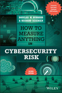
In 2022, Seiersen conducted the same exercise as Kent. In this case, just over 100 security executives from leading organizations were asked to assess the same probability statements. As you can see from Figure 5.2, the results are considerably worse than those found in Figure 5.1.
In our survey, 28% of cybersecurity professionals reported that they use verbal or ordinal scales where the probability they are meant to represent is not even defined. However, some scale users attempt to manage this ambiguity by offering specific definitions for each point. For example, “Very unlikely” can be defined as a probability of less than 10%. (In fact, this is what NIST 800–30 does).6 In our survey, 63% of respondents who use ordinal scales indicated that they use verbal or numbered ordinal scales where the probabilities are defined in this way. However, Budescu finds that offering these definitions doesn't help, either.

FIGURE 5.1 Variations of NATO Officers’ Interpretations of Probability Phrases
Source: Adapted from Heuer 1999.
FIGURE 5.2 Variations of Security Leaders’ Interpretations of Probability Phrases
TABLE 5.2 Variance in Understanding Selected Common Terms Used to Express Uncertainty in the IPCC Report
Source: Adapted from [3].
| Examples of Some Likelihood Terms Used in the Report | IPCC Guidelines for Meaning | Minimum of All Responses | Maximum of All Responses | Percentage of Responses That Violated Guidelines |
|---|---|---|---|---|
| Very likely | More than 90% | 43% | 99% | 58% |
| Likely | Between 66% to 90% | 45% | 84% | 46% |
| Unlikely | Between 10% and 33% | 8% | 66% | 43% |
| Very unlikely | Less than 10% | 3% | 75% | 67% |
Even in situations where each of the verbal scales was assigned specific probability ranges (e.g., “Very likely” was defined as “Greater than 90%” and “Very unlikely” was defined as “Less than 10%”), these rules were violated over half the time. In other words, even when participants were told exactly what the terms meant, they interpreted the terms in the context of the statement they were presented in. In that way, the phrase “Very likely” meant something different to the subjects when it was in the context of temperature extremes, glaciers melting, or sea level rise.
Table 5.2 shows how widely the subjects in Budescu's study interpreted these verbal scales even when they were given specific directions regarding what they meant. It appears that about half of respondents ignored the guidelines (perhaps the term “guideline” itself invited too much interpretation).
Some of the more extreme results beg for further explanation. In the case of “very unlikely” we see a remarkable range of 3–75%. The 75% isn't just a single outlier, either, since two‐thirds of the respondents violated the guideline (meaning they interpreted it to mean something greater than 10%). How could this be? Budescu found very little relationship between the subjects’ probability interpretations and their predisposition on climate research (i.e., they did not simply put higher probabilities on events if they indicated more concern about climate research). But he did point out that the ambiguity of some of the statements might have had some bearing on responses. If the statement was about the likelihood of “heat extremes,” the user may have included uncertainty about the meaning of “heat extremes” when they assessed a probability.
Hubbard has another potential explanation. Anecdotally, he has observed conversations about risks with clients where something was judged “highly likely” in part because of the impact it would have. Of course, impact and likelihood are supposed to be judged separately, but managers and analysts have been heard making statements like “A 10% chance per year is far too high for such a big event, so I think of 10% as highly likely.” This is purely anecdotal, of course, and we don't rely on these sorts of observations—the data from Budescu and Kent is sufficient to detect the problem. But in terms of potential explanations, the fact that such statements have been observed at least introduces a possibility: Some users of these terms are attempting to combine likelihood, impact, and their own aversion to risk in highly ad hoc ways. These users require methods that unpack these distinct concepts.
Furthermore, to adequately define a probability of an event, we can't exclude the time period it is meant to cover. If, for example, we say that an event is 10% likely, do we mean there is a 10% chance of it happening sometime next year or sometime in the next decade? Obviously, these would be very different estimates. How is it that management or analysts could come to agree on these points when they haven't even specified such a basic unit of measure in risk?
All these factors together combine to create what Budescu refers to as the “illusion of communication.” Individuals may believe they are communicating risks when they have very different understandings of what is being said. They may believe they have come to an agreement when they all say that one risk is “medium” and another is “high.” And even when specific numbers are presented for probabilities, the listener or the presenter may conflate their own risk tolerance with the assessment of probability, or they may be assuming that the probability is for an event over a longer time period than someone else is assuming it to be.
So far, we have only discussed the psychology of how people interpret ambiguous terminology in regard to risk, but that is not the end of it. Separate from the use of nonquantitative labels for probabilities or the consequences of other ambiguities, there are some curious human behaviors that arise in their responses to subjective ordinal scales in general. Relatively arbitrary features of the scale have a much larger effect on judgment than the users would expect.
For example, Craig Fox of UCLA co‐authored several studies showing that arbitrary features of how scales are partitioned have unexpected effects on responses, regardless of how precisely individual values are defined.7 On a scale of 1 to 5, the value of “1” will be chosen more often than if it were a scale of 1 to 10, even if “1” is defined identically in both (e.g., “1” could mean an outage duration of less than 10 minutes or a breach resulting in less than $100,000 in losses). In addition, there is plenty of research showing how other arbitrary features of scales affect response behavior in ways that are unexpected and larger than you might think. These include whether ordinal numbers are provided in addition to verbal scales or instead of them,8 or how the direction of the scale (5 is high or 5 is low) affects responses.9
There are several risk matrix standards that apply a verbal description of a likelihood and provide a specific quantity or interval it should represent. For example, one common method defines one of the likelihood categories as “Has been heard of in the industry” or “Happens frequently in the organization” to refer to the risk of a specific event for a particular asset. In addition, a specific quality like 10% or maybe a range of 2% to 20% is given as an additional guideline. This just confuses things further.
Hubbard is often asked to evaluate existing risk management methods in organizations both inside and outside of cybersecurity, some of which use risk matrices like this. He observes that in the petroleum industry or utilities where he has seen this method, the phrase “Has been heard of” might refer to the past 10 or 20 years or longer, and it could mean it happened once or a few times among some number of assets, such as oil refineries or power plants. Also, if the event happened once in the last five years, it matters whether that was once among 10 similar facilities in the industry or thousands.
Depending on how these terms are interpreted and how many examples of that type of asset exist in the industry, Laplace's rule of succession (from Chapter 2) might show a likelihood of less than one in a thousand per year for a given asset or more than one in ten per year. Hubbard found that, invariably, different managers in the same organization made different assumptions about what “Has been heard of in the industry” meant. Some said they paid no attention to the quantity and only used the verbal description for guidance, while others assumed that everyone used the quantities. In large organizations, different risks for different assets were evaluated by different individuals. So whichever risks made the “Top 10” was mostly a function of which individuals judged them.
The possibilities of varied interpretations are fairly standard considerations in the field of psychometrics and survey design. Surveys are designed with various sorts of controls and item testing so that the effects of some biases can be estimated. These are referred to as “artifacts” of the survey and can then be ignored when drawing conclusions from it. But we see no evidence that any of these considerations are ever entertained in the development of risk scales. We need to consider the psychology of how we assess risks and how we use these tools. As Richard Heuer urged, this cannot be taken for granted.
Intelligence analysts should be self‐conscious about their reasoning process. They should think about how they make judgments and reach conclusions, not just about the judgments and conclusions themselves.
—Richards J. Heuer Jr., Psychology of Intelligence Analysis
How the Risk Matrix Doesn't Add Up
At first glance, the math behind a risk score or risk matrix could hardly be simpler. But, as with the psychology of scales, further investigation reveals new concerns. This may seem like a bit of esoterica, but, just as with every other component of risk analysis, the scale of the problem means we shouldn't leave such a widely used tool unexamined.
Perhaps nobody has spent more time on this topic than Tony Cox, PhD, an MIT‐trained risk expert. He has written extensively about the problems that ordinal scales introduce in risk assessment and how those scales are then converted into a risk matrix (which is then often converted into regions of “low” to “high” risk). He investigates all the less‐than‐obvious consequences of various forms of ordinal scales and risk matrices and how they can lead to decision‐making error.10
One such error is what he refers to as “range compression.” Range compression is a sort of extreme rounding error introduced by how continuous values like probability and impact are reduced to a single ordinal value. No matter how the buckets of continuous quantities are partitioned into ordinal values, choices have to be made that undermine the value of the exercise. For example, the upper end of impact may be defined as “losses of $10 million or more” so that $10 million and $100 million are in the same bucket. To adjust for this, either the $10 million must be increased—which means the ranges in the lower categories also must be widened—or the number of categories must be increased.
Range compression is further exacerbated when two ordinal scales are combined onto a matrix. Cox shows how this can result in two very different risks being plotted in the same cell (i.e., the position at a given row and column in a matrix) and how a higher‐risk cell can contain a risk that is lower than a risk in a low‐risk cell. To see this, consider the risk matrix shown in Table 5.3. It is drawn from an actual risk matrix example promoted by a major consulting organization.
First, let's look at how two very different risks can end up in the same cell. We'll plot two risks in the “Seldom” likelihood category, which ranges from “greater than 1% and up to 25%” to the maximum loss category, “$10 million or more.” The two risks are:
TABLE 5.3 Risk Matrix Example to Illustrate Range Compression Problems
| Impact | |||||||
| Negligible | Minor | Moderate | Critical | Catastrophic | |||
| <$10K | $10K to <$100K | $100K to <$1 million | $1 million to <$10 million | ≥$10 million | |||
| Likelihood | Frequent | 99%+ | Medium | Medium | High | High | High |
| Likely | >50%–99% | Medium | Medium | Medium | High | High | |
| Occasional | >25%–50% | Low | Medium | Medium | Medium | High | |
| Seldom | >1%–25% | Low | Low | Medium | Medium | Medium | |
| Improbable | ≤1% | Low | Low | Low | Medium | Medium | |
- Risk A: likelihood is 2%, impact is $10 million;
- Risk B: likelihood is 20%, impact is $100 million.
With this information Cox computes the “expected loss” (probability‐weighted loss), just as an actuary would do for many types of risks. He compares the products of the likelihoods and impacts of the risks: $200,000 for risk A (2% × $10 million) and $20 million for risk B (20% × $100 million). In other words, to an actuary, risk B would be considered to have 100 times the risk of risk A. Yet these two very different risks would actually be plotted in the same cell (that is, same row, same column) on a risk matrix!
Next, let's look at how Cox shows that two very different risks can be plotted in cells that are the opposite order by expected loss. Again, this relies on the fact that in order to map continuous values with wide ranges to discrete bins, some “bins” on the likelihood and impact axes have to contain wide ranges of values. Here are another two risks:
- Risk A: Likelihood is 50%, impact is $9 million;
- Risk B: Likelihood is 60%, impact is $2 million.
In this case, risk A has an expected loss of $4.5 million, and risk B has an expected loss of $1.2 million. Yet, if we followed the rules of this matrix, risk B is considered a “High” risk, and risk A is only “Medium.” This is what is called a “rank reversal” and it is not just an academic problem. Hubbard has been asked to audit risk management methods in many industries both within and outside of cybersecurity and he finds many examples of rank reversal among actual risks identified by organizations. Cox says that these properties combine to make a risk matrix literally “worse than useless.” As remarkable as this sounds, he argues (and demonstrates) it could even be worse than randomly prioritized risks.
Some might argue that this is a straw man argument because we don't usually have the specific probabilities and impacts used in these examples. We only have vague ideas of the ranges, they might argue. But the ambiguity hides problems instead of facilitating the lack of information. Cox also points out that risk matrices ignore factors such as correlations between events. He stated in an interview with this book's authors that “it is traditional to completely ignore correlations between vulnerability, consequence, and threat. Yet, the correlations can completely change the implications for risk management.”
Like the authors, Cox sees the potential for conflation of computed risks and risk tolerance: “The risk attitude used in assessing uncertain consequences is never revealed in conjunction with the risk matrix. But without knowing that, there is no way to decipher what the ratings are intended to mean, or how they might change if someone with a different risk attitude were to do the ratings. The assessments shown in the matrix reflect an unknown mixture of factual and subjective components.” He asks what seems like a basic question: “The problem arises when you ask, ‘What did I just see?’ when looking at a score or matrix.”
The reader could make the case that this is just a feature of this particular risk matrix, and a different matrix with different categories wouldn't have this problem. Actually, there will still be examples of inconsistencies like this regardless of how the ranges are defined for impact and likelihood. Cox himself even worked on how some of these issues can be avoided—but only some. Cox's “risk matrix theorem” shows how certain rules and arrangements of categories can at least lead to a weakly consistent matrix. He defines “weakly consistent” in a very specific way and never concedes that a matrix could be entirely consistent. In short, matrices are ambiguity amplifiers. Cox summarizes his position for us by saying, “Simply on theoretical grounds there is no unambiguous way of coming up with such ratings in a risk matrix when the underlying severities are uncertain.”
Other scoring methods don't necessarily rely on risk matrices. As mentioned earlier, methods such as OWASP simply add up multiple ordinal scales to get to an overall risk score. We also noted that this method and others like it in security are used in various scoring systems including the Common Vulnerability Scoring System (CVSS), the Common Weakness Scoring System (CWSS), and the Common Configuration Scoring System (CCSS). All of these scoring systems do improper math on nonmathematical objects for the purpose of aggregating some concept of risk. These wouldn't have the same problems as a risk matrix, but they introduce others—such as the mathematical no‐no of applying operations like addition and multiplication to ordinal scales. As the authors have stated it in presentations on this topic, it is like saying “Birds times Orange plus Fish times Green equals High.” And, of course, methods like those used in the CVSS would share the same problems of scale‐response psychology (discussed earlier) as any risk matrix.
Amplifying Effects: More Studies Against the Risk Matrix (as If We Needed More)
The effects mentioned so far are compounding, meaning they work together to make risk management even more difficult than they could individually. Work from multiple sources has been done that shows the harm of combining scales and risk matrices.
In 2008 and 2009, Hubbard collected data from five different organizations regarding cybersecurity risks. Each provided separate responses from multiple individuals, with each individual providing dozens of scores for various risks. In total, there were a little over 2,000 individual responses. Hubbard found that the responses were highly clustered—about 76% of responses fell within just two values on the scale (a 3 or 4 on a 5‐point scale). That is, most of the responses really boiled down to a decision between two specific values on the 5‐point scale. What was meant to be a 5 × 5 matrix was mostly a 2 × 2 matrix. The net effect of the clustering was an even lower resolution—that is, an even bigger rounding error and even less information. Combined with the other research, Hubbard suspected this clustering could only exacerbate the problems found in the earlier research.
Hubbard teamed up with psychologist Dylan Evans to publish these findings in the IBM Journal of Research & Development. Evans is an experienced researcher and professor who had also researched the effects of placebos and their use in clinical drug trials. Their paper, which was published in 2010, presented a comprehensive review of the literature up to that point and combined those findings with Hubbard's observations from his collection of ordinal‐scale responses. In short, the paper concluded:
The problem discussed in this paper is serious. The fact that simple scoring methods are easy to use, combined with the difficulty and time delay in tracking results with respect to reality, means that the proliferation of such methods may well be due entirely to their perceived benefits and yet have no objective value.11
Another more recent and (as Hubbard is happy to concede) even more comprehensive investigation, using psychological literature, theoretical issues, and original data, found similar results. In Economics & Management journal of the Society of Petroleum Engineers, authors Philip Thomas, Reidar Bratvold, and J. Eric Bickel reviewed 30 different papers that described various risk matrices, mostly used in the oil and gas industry. In addition to providing a comprehensive review of all the literature (including Budescu, Cox, Hubbard and Evans, and many more), the authors also examined the effect of changing the design of the risk matrix and the ranking of various risks, and then measured how risk matrices distort data.12
Leveraging Cox's findings, Thomas and his colleagues showed how the designs of these various risk matrices affected the rankings of risks in a way the matrices’ designers probably did not anticipate. For example, 5 of the 30 risk matrix designs they investigated reversed the score—that is, 1 was high impact or likelihood instead of 5. These matrices would then multiply the likelihood and impact scores just as many of the other matrices did, but the lower product was considered high risk. The designers of these methods may have thought this was an arbitrary choice that would have no consequence for the risk rankings. Actually, it changed them a lot. Thomas also looked at how various methods of categorizing likelihood and impact into a few discrete ordinal values (such as defining “Unlikely” as 1% to 25% or moderate impact as $100,000 to $1 million) modified risk rankings. Again, they found that these arbitrary design choices had a significant impact on ranking risks.
Thomas and colleagues also estimated a “lie factor” for each of several types of risk matrices. The lie factor is a measure defined by Edward Tufte and Peter Graves‐Morris in 1983 based on how much data is distorted in a chart by misleading features of the chart, intentional or otherwise.13 This is effectively a variation on the “range compression” that Cox examined in detail. Using a particular method for computing the lie factor, they found that the ratio of distortions of data averaged across the various risk matrix designs was in excess of 100. To get a sense of what a lie factor of 100 means, consider that when Edward Tufte explained this method, he used an example that he classified as a “whopping lie”—it had a lie factor of 14.8.
Thomas found that any design of a risk matrix had “gross inconsistencies and arbitrariness” embedded within it. Their conclusion is consistent with the conclusions of everyone who has seriously researched risk matrices:
How can it be argued that a method that distorts the information underlying an engineering decision in non‐uniform and uncontrolled ways is an industry best practice? The burden of proof is squarely on the shoulders of those who would recommend the use of such methods to prove that the obvious inconsistencies do not impair decision making, much less improve it, as is often claimed.
They presented these findings in a webinar that was part of Stanford's Strategic Decision and Risk Management lecture series. To drive home their finding, one of the PowerPoint slides in their presentations contained a large rectangular space titled “Heat Map Theory and Empirical Testing” (see Figure 5.3). Showing a little humor combined with a lot of seriousness, the rectangle was empty.
Again, if you are wondering whether these findings must somehow be limited to the oil and gas industry (the target audience of the journal where this research was published), consider the NASA example briefly mentioned in Chapter 4. Recall that the research showed how Monte Carlo and statistical regression–based methods performed compared to “softer” methods. The softer method referred to was actually NASA's own version of the 5 × 5 risk matrix. The mission scientists and engineers arguably had a subject‐matter advantage over the accountants—and yet, the accountants using Monte Carlo simulations and historical data were better at forecasting than the scientists and engineers using a risk matrix.
Last, these scales do not account in any way for the limitations of expert judgment as described in Chapter 4. The errors of the experts are simply further exacerbated by the additional errors introduced by the scales and matrices themselves. We agree with the solution proposed by Thomas, Bickel and Bratvold. There is no need for cybersecurity (or other areas of risk analysis that also use risk matrices) to reinvent well‐established quantitative methods used in many equally complex problems. Thomas et al. recommend proper decision‐analysis tools that use explicit probabilities to represent uncertainty. They compare RMs (risk matrices) to decision analysis in this way:
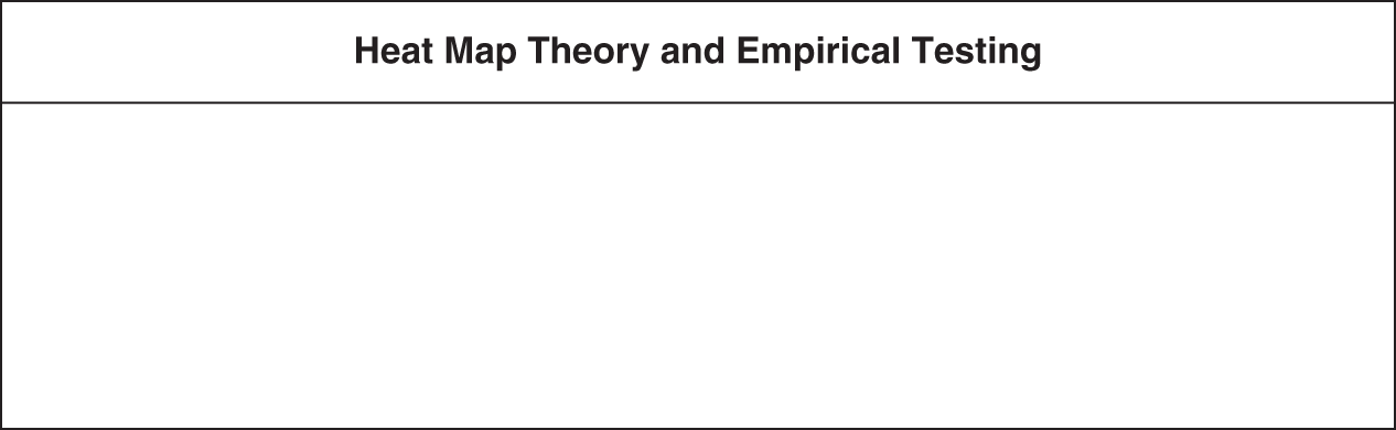
FIGURE 5.3 Heat Map Theory and Empirical Testing
Source: Adapted from [12].
[T]he processes and tools drawn from decision analysis are consistent, do not carry the inherent flaws of the RMs, and provide clarity and transparency to the decision‐making situation. Our best chance for providing high‐quality risk‐management decisions is to apply the well‐developed and consistent set of processes and tools embodied in decision science.
To make this distinction clear, just compare the risk matrix to the loss exceedance curve presented in Chapter 3. Recall that the LEC captures all uncertainty about impact regardless of how wide the range might be, and that the risk tolerance curve provides an explicit record of how much risk an organization's management accepts. So how does the risk matrix allow for more uncertainty about impact if impact doesn't neatly fit in one category? How does the risk matrix unambiguously capture the risk tolerance of management in a way that allows for clear evaluation of options?
Like the authors of this book, Thomas, Bratvold, and Bickel state what should now be the obvious conclusion for anyone who considers all the research:
Given these problems, it seems clear that RMs should not be used for decisions of any consequence.
Hopefully, that settles that.
Exsupero Ursus and Other Fallacies
You might have heard the old joke about two hikers getting ready for a walk into the woods. (If you have heard it—probably many times—thanks in advance for your indulgence, but there is a point.) One hiker is wearing his running shoes instead of his regular hiking boots. The other asks, “Is there something wrong with your regular boots?” to which the first hiker responds, “No, I just heard there were bears in the woods today. I wore these shoes so I could run faster.”
His friend, confused, reminds him, “But you know you can't outrun a bear.”
The hiker with the running shoes replies, “I don't have to outrun a bear. I just have to outrun you.”
This old (and admittedly tired) joke is the basis for the name of a particular fallacy when it comes to evaluating models or decision‐making methods of any kind. We call it the Exsupero Ursus fallacy—or, if you can do without the hokey pseudo‐scholarly Latin term we just made up with Google Translate, you can call it the “beat the bear” fallacy. The basis of this fallacy goes something like this: If there is a single example of one method failing in some way or even having a minor weakness, we default to another method without ever investigating whether the alternative method has even more weaknesses and an even worse track record.
We get many opportunities to meet managers and executives who have difficulty believing that quantitative models could possibly be an improvement over expert intuition or qualitative methods. One such person was an operational risk officer who challenged quantitative methods by asking, “How can you possibly model all the factors?” Of course, models never model or even attempt to model “all” the factors. The risk officer was committing the Exsupero Ursus fallacy. Does he believe that when he uses his own judgment or a softer score‐based method that he is capturing literally all the factors? Of course not. He was simply comparing the quantitative method to some ideal that apparently captures all possible factors as opposed to comparing quantitative method to the actual alternatives: his own judgment or other methods he preferred.
Remember, the reason we are promoting the quantitative methods mentioned in this book is that we can point to specific research showing that they are superior ‐ that is, measurably superior ‐ to specific alternatives like expert intuition. As the great statistician George Box is often quoted as saying, “All models are wrong, but some are useful.” And to take it further, the research clearly shows that some models are measurably more useful than others. That is, they predict observed results better and are more likely to lead to preferred outcomes. When someone points out a shortcoming of any model, the same standard must then be applied to the proposed alternative to that model. The first model may have error, but if the alternative has even more error, then you stick with the first.
What we've been calling the Exsupero Ursus Fallacy for years is related to what some researchers call the “Algorithm Aversion.”14 Berkeley Dietvorst at the University of Chicago along with Joseph P. Simmons and Cade Massey from Wharton conducted experiments where subjects were asked to make estimates related to the performance of graduate students based on undergraduate performance data and the ranking of airport traffic by state based on various other demographic and economic data. The subject could choose whether they were going to use an algorithm to generate their estimates or rely on human judgment. They were rewarded for accurate estimates, so they were incentivized to choose which approach would be more accurate. In some cases, they were shown performance data for the humans, the algorithms, or both before they had to choose which to rely on for their own estimates. Some were shown no previous performance data on the algorithms of humans.
Averaged across multiple experiments, 62 percent chose the algorithms when shown no data on past performance or only the data on humans. But for those who were shown data on past performance of algorithms, those who chose the algorithms dropped by almost half (down to 32 percent), even though the human estimates had more error than the algorithms. In all the experiments, the subjects who chose the algorithms made more money than those who didn't. The researchers concluded that many subjects were just more intolerant of error from algorithms than error from humans. In other words, they had a double standard. They expected better performance from algorithms, but when they saw the algorithms had any error, they rejected the algorithms in favor of the clearly inferior alternative. Algorithm aversion research is confirmation of the pervasiveness of the Exsupero Ursus fallacy. This fundamental fallacy seems to be behind several arguments against the use of quantitative, probabilistic methods. We only need to list a few, and you will see how each of the objections can be countered with the same response.
Beliefs about the Feasibility of Quantitative Methods: A Hard Truth
Some cybersecurity experts in the survey (18%) said they agreed with the statement “Ordinal scales must be used because probabilistic methods are not possible in cybersecurity.” This can be disproven by virtue of the fact that every method we discuss in this book has already been used in real organizations many times. Holding a belief that these methods are not practical is sort of like telling an airline pilot that commercial flight isn't practical. So where does this resistance really come from?
Our survey indicated one potential reason behind that position: statistical literacy is strongly correlated with acceptance of quantitative methods. One set of questions in the survey tested for basic understanding of statistical and probabilistic concepts. We found that those who thought quantitative methods were impractical or saw other obstacles to using quantitative methods were much more likely to perform poorly on statistical literacy.
The statistical literacy section of the survey had 10 questions related to basic statistical literacy. Many of those survey items were based on questions that had been used in other surveys on statistical literacy by Kahneman and others. Some of the questions involved common misunderstandings of correlation, sample size, inferences from limited data, the meaning of “statistically significant,” and basic probabilities (see example in Table 5.4).
For further details, we put the entire survey report available for download on www.howtomeasureanything.com/cybersecurity.
TABLE 5.4 Example Stats Literacy Question
| Assume the probability of an event, X, occurring in your firm sometime in 2016 is 20%. The probability of this event goes to 70% if threat T exists. There is a 10% probability that threat T exists. Which of the following statements is true? |
| A. If the threat T does not exist, the probability of the event X must be less than 20%.* |
| B. If the event X does not occur, then T does not exist. |
| C. Given that the event X occurs, the probability that threat T exists must be greater than 50%. |
| D. There is insufficient information to answer the question. |
| E. I don't know. |
* Correct answer. (Chapter 8 covers the relevant rules—specifically rule 6.)
We then compared stats literacy to the attitudes regarding the seven strongly anti‐quantitative questions in the ATQM section of the survey. A summary of the relationship between stats literacy and positive attitudes toward the use of quantitative methods is shown in Figure 5.4.
Note that a rating in the “Median or Lower” group on pro‐quant attitude doesn't necessarily mean they were generally against quantitative methods. Most people were quite supportive of quantitative methods, and so the median number of supportive responses is still more supportive than not, although it shows more reservations about quantitative methods than those who had more than the median number of pro‐quant responses. For stats literacy, however, a median score (3 out of 10) was about how well someone would do if they were guessing (given the number of choices per question, randomly choosing any answer other than “I don't know” would produce 2.3 correct out of 10, on average). Those who did significantly worse were not just guessing; they frequently believed in common misconceptions.
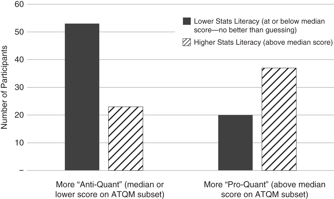
FIGURE 5.4 Stats Literacy versus Attitude toward Quantitative Methods
As Figure 5.4 shows, those who scored above the median on stats literacy were much more likely to be above the median on “pro‐quant” attitudes; likewise, those who were pro‐quant were more likely to be stats literate. This is true even for what may seem like a small number of questions in this quiz.
Given the number of questions and the number of potential choices per question, we can apply certain statistical tests. We find that—when we do the math—the relationship between stats literacy and pro‐stats attitudes is statistically significant even with the small number of questions per respondent. (For the particularly stats‐literate among the readers, these findings have a P‐value of less than 0.01.) The survey also provided some other interesting observations. Here are a few of them:
- The most anti‐quantitative quartile of subjects (the bottom 25%) were twice as likely to simply skip the stats literacy quiz as those who were in the most pro‐quant quartile.
- More experience in cybersecurity was associated with positive attitudes toward quantitative methods. It also appears that those who had even tried quantitative methods, such as Monte Carlo simulations, were much more likely to be pro‐quantitative. We found that 23% of the more pro‐quant group had tried Monte Carlo simulations, while only 4% of the anti‐quantitative group had done so. We aren't saying that the pro‐quantitative disposition drove the desire to try Monte Carlo simulations or that trying Monte Carlo made them pro‐quantitative. But the association is strong.
- Those who performed the worst on the stats literacy quiz were more likely to overestimate their skills in statistics. This is consistent with a phenomenon known as the Dunning‐Kruger effect.15 That is, there is a tendency for people who perform poorly on any test (driving, basic logic, etc.) to believe they are better than they are at the measured task. In our survey we found that 63% of individuals with below‐average statistics literacy wrongly identified themselves as having average or above‐average proficiency in statistics. So those who are performing poorly on stats literacy won't usually know they have misconceptions.
All this just confirms with empirical analysis the suspicions we've had based on multiple anecdotal observations. Those who believe quantitative methods are impractical in cybersecurity are not saying so because they know more about cybersecurity but because they know less about quantitative methods. If you think that you understand quantitative probabilistic methods but do not agree that these methods are feasible in cybersecurity, don't shoot the messenger. We're just reporting the observation. For those of you in the majority who believe better methods are feasible and are supportive of exploring them, we don't mean to preach to the choir. Perhaps you can use this information to diagnose internal resistance and possibly influence future training and hiring decisions to address unfamiliarity with quantitative methods in cybersecurity.
It may be a hard pill to swallow for some, but the conclusion from our survey is as unavoidable as it is harsh. Cybersecurity is a critically important topic of growing concern and we don't have the luxury of pulling punches when solving this problem. As we argued in Chapter 4 as well as earlier in this chapter, all models should be critically evaluated, including quantitative solutions, so it is not our objective to browbeat these voices into silence. But blanket objections to quantitative methods need to be recognized as nothing more than stats‐phobia—born of stats illiteracy.
Since the first edition of this book, we have gotten some emails on this point and we will continue to get them with this edition. But the math is sound and the arguments against the conclusion will contain critical flaws (we know this because we have already seen many of them). The person at Hubbard Decision Research who assisted with this analysis was one of HDR's senior quantitative analysts, Jim Clinton. He has a PhD in cognitive psychology and has published scientific research specializing in the application of advanced statistical methods to experimental psychology. So, yes, he knows what he is doing when he is assessing the statistical validity of a survey. We mention this in anticipation of objections to the survey methods, the number and type of questions we used, and the overall statistical significance. The methods, the sample size, and the correct answers to the stats literacy questions are all quite sound. But we know from past experience and the results of this survey that there will be some people who—based on an incorrect belief of their understanding of statistical methods—presume that because the findings contradict the math they do in their heads, it must be the survey that was wrong. It's not. We didn't do the math in our heads. We did the actual math. Now let's continue.
Same Fallacy: More Forms
The 29% who agreed with the statement “Ordinal scales or qualitative methods alleviate the problems with quantitative methods” were committing a type of Exsupero Ursus fallacy. The thinking here is that because quantitative methods are imperfect, we must use the alternative, which somehow corrects for these errors. But what is this alleged mechanism of correction? From what we see of the research previously presented, not only do ordinal scales and risk matrices not correct for the errors of quantitative methods, they add errors of their own.
Again, we believe we should always ask tough questions of any method, including quantitative ones, and we've attempted to address this by citing overwhelming research to make our point. But we also apply the same skepticism to the preferred, softer alternatives promoted by so many standards organizations and consulting firms. We cited research that consistently finds flaws in these methods and finds a relative advantage in quantitative methods.
“Probabilistic methods are impractical because probabilities need exact data to be computed and we don't have exact data” is a related and common objection to the use of statistics in many fields, not just cybersecurity. In our survey, 23% of respondents agreed with the statement. Yet, as we mentioned in Chapter 2, you have more data than you think and need less than you think, if you are resourceful in gathering data and if you actually do the math with the little data you may have. The Exsupero Ursus fallacy here, again, is that the alternative to the proposed quantitative method somehow alleviates the lack of data. On the contrary, it appears ordinal scales and expert intuition may be useful in obfuscating the lack of data because they gloss over the entire issue. Again, the previous research shows that ordinal scales and risk matrices might actually add error—that is, they literally reduce the limited information available to the intuition of the person using them.
Fortunately, like the other anti‐quant‐attitude questions, most respondents disagreed. They are more willing than not to try better methods. However, 23% is a significant portion of cybersecurity professionals who have a fundamental misunderstanding of why probabilistic methods are used. One of those who agreed with the statement wrote the following in an open‐ended response section of the survey:
The problem I have always had with quantifying a security risk is that when you have a vulnerability, say, an unpatched server, there is such a wide range of things that could happen if that was to be exploited … So, what does it mean to go to your board and say, well, this could result in a loss in the range of $0–$500 million?
Before we respond, know that this is not a personal attack on anyone—not the person who graciously participated in our survey or anyone else who agrees with the statement. But we aren't helping cybersecurity by not providing an honest evaluation of the claim. We respect this claim enough to say it deserves a response. So here we go.
Of course, such losses are at least possible for organizations that are large enough, since we know of losses about that size that have happened in business. So, if this is the “possibility range,” then why not make the upper bound a billion dollars or more? But clearly these outcomes are not all equally likely. In contrast, a probability distribution communicates the probabilities of various outcomes. We suspect that this analyst has more information than this or could at least gather more information.
If that enormous range really is the extent of uncertainty about this loss, and if everything in that range was equally likely, how does the analyst propose that, say, a conventional risk matrix would have alleviated that uncertainty? Of course, it would not. It would simply have glossed over the uncertainty. (In fact, the analyst probably would have plotted this risk in a single cell of the matrix, even though the stated range would have spanned most or all of the impact categories.)
Another interesting question is that if this were really the level of uncertainty about potential losses, then what steps is the analyst taking to reduce that uncertainty by at least some amount? Surely, any risk with such a wide range of uncertainties would merit further investigation. Or does this analyst plan on simply continuing to hide this major uncertainty from the board by using ambiguous risk terminology? Remember from Chapter 2 that it is in precisely these cases of extreme uncertainty where uncertainty reduction is both easier and most valuable. We have already presented research on how decomposing a wide range like that (by thinking through estimates of individual consequences and running a simulation to add them up) is likely to reduce uncertainty.
Those who agree with the statement that probabilistic methods need exact data misunderstand a basic point in probabilistic methods. We use quantitative, probabilistic methods specifically because we lack perfect information, not in spite of it. If we had perfect information, we would not need probabilistic models at all. Remember, nothing we are proposing in this book is something the authors and other colleagues haven't done many times in many environments. We have presented wide ranges many times to upper management in many firms, and we find they appreciate explicit statements of uncertainty.
We can make a similar response to the concern that cybersecurity is too complex to model quantitatively or that quantitative methods don't apply where human opponents are involved. Just like the previous questions, we have to ask exactly how risk matrices and risk scores alleviate these issues. If it is too complex to model quantitatively, how do we propose that a nonquantitative solution addresses this complexity? Remember, no matter how complex a system is, if you are making even purely subjective judgments about the system, you are modeling it. The Exsupero Ursus fallacy (i.e., it's not a perfect method; it failed once before, so I can't use it) still depends on failing to apply the same standard to the alternatives to probabilistic methods.
Many experts make an incorrect assumption that the more complex the problem, the worse quantitative methods will do compared to human experts. Yet, the findings of Meehl and Tetlock (reviewed in Chapter 4) show that as problems get more complex, the human experts are not doing better compared to even naive statistical models. So the complexity of the world we model is common to both quantitative and nonquantitative models. But, unlike the risk matrix and ordinal scales, the components of even a simplified quantitative method hold up to scientific scrutiny.
Christopher “Kip” Bohn, an experienced actuarial consultant, runs into this same objection and has the same reaction we do. Bohn has done a wide variety of risk analysis in many fields and is one of a growing rank of actuaries who have been working on underwriting cybersecurity risks using the quantitative tools of analytics. He describes his response in an interview:
In every single presentation I give in analytics I have a slide regarding how to respond to people who say you can't model that. Of course, they are actually building a model in their head when they make a decision. I tell them, “We just want the model out of your head.”
Well said, Kip. Complexity, the lack of data, unpredictable human actors, and rapidly changing technology are often used as excuses for not adopting more quantitative methods. Ironically, the de facto solution is often to somehow deal with these issues in the undocumented and uncalculated intuition of the expert. If a problem is extremely complex, that's exactly the time to avoid trying to do it in your head. Aerodynamic simulations and power plant monitoring are also complex. But that is exactly why engineers don't do that analysis their heads. Cybersecurity will deal with multiple, interacting systems and controls and multiple types of losses. Some of these systems will have different types of losses than others, and some events are more likely than others. Then you have to roll it up into a portfolio to determine overall risk. It's not particularly hard math (especially since we are providing spreadsheets for just about every calculation we talk about), but you still don't want to do that math in your head.
So whenever you hear such an objection, just ask, “But how does your current method (risk matrix, ordinal scores, gut feel, etc.) alleviate this shortcoming?” It only feels like the issue is addressed in softer methods because the softer methods never force you to deal with it. And if you are uncertain—even as uncertain as the $0 to $500 million impact range mentioned earlier—then you can specifically state that uncertainty and prioritize your security controls accordingly.
The Target Breach as a Counter to Exsupero Ursus
A final objection we will mention related to Exsupero Ursus is that there are numerous examples of quantitative methods failing, and it is therefore argued that they should be avoided. The idea is that events such as the 2008 financial crisis, the 2010 Deepwater Horizon rig explosion and oil leak in the Gulf of Mexico, the 2011 Fukushima Nuclear Power Plant disaster in Japan, the COVID pandemic of 2020 to 2022 and other events indicated the failure of quantitative methods. There are several problems with this objection, which Hubbard also discusses in The Failure of Risk Management, but we will summarize a couple of them.
First, the anecdotes presume that an actual quantitative method was being used instead of intuition and if intuition were used it somehow would have averted the disaster. There is no basis for this claim, and there is actually evidence that the opposite is true. For example, greed and incentives created and then obscured the risks of investments, and in some cases (such as the AIG crisis) it was in fact the lack of actuarially sound analysis by regulators and auditors that allowed these systems to flourish.
The second problem with this objection is that they are selected anecdotes. How many examples of failures are there from methods based on pure intuition or soft methods? Even if these were legitimate examples of actual quantitative‐method failure (the authors would concede there are many), we still come back to how to avoid the basic fallacy we are discussing—that is, we need to compare them to the failure rate of nonquantitative methods. The fact is there are also many failures where nonquantitative methods were used in decision making. Indeed, how well did judgment and intuition perform in the financial crisis, the design of the Fukushima plant, or the management of Deepwater Horizon?
The massive data breach of the retailer Target in 2013 is a case in point. This breach is well known in the cybersecurity community, but perhaps what is less widely known are the methods Target used and failed to use to assess its risks. Hubbard and Seiersen interviewed a source who was employed by Target up to about a year before the event. According to our source, Target was about as far from a quantitative solution to cyber risks as any organization could be. Even though there were attempts to introduce more quantitative methods, several people were entrenched in using a method based on assessing risks based on verbal “high, medium, and low” labels. There were executives who believed quantitative methods to be too complex and that they required too much time. They actually took the trouble to create a list of reasons against using quantitative methods—the items on the list that we know about are those very objections we have been refuting in this chapter. (We were told that since the breach, there has been a significant change in cybersecurity leadership.)
Eventually the company recognized that credit card records of as many as 70 million people had been breached. The combined settlements to Master Card and Visa exceeded $100 million.16 Now, if we believed anecdotes were a sufficient basis for a comparison of methods, then we could definitely spend the time to find more examples. After all, were Anthem, Sony, Home Depot, the US federal government, and other organizations that were hit by major cyberattacks using probabilistic methods instead of scales and risk matrices? We doubt it.
Of course, selected anecdotes are not the way to support the claim about which method is better. As we have done so far, the only way to properly avoid the Exsupero Ursus fallacy is to look at large sets, chosen in an unbiased manner, and systematically compare failures of both methods. Even if one method has failures, it should be preferred over a method that has even more. The research we presented so far (see the endnotes for this chapter and Chapter 4) supports the claim that quantitative methods outperform human expert intuition and humans using scales or risk matrices. The only research available on risk matrices, on the other hand, supports the claim that risk matrices do no good at all and may even do harm.
Communication and Consensus Objections
Last, there are objections that are neither strictly Exsupero Ursus fallacies nor based on misconceptions about quantitative methods such as the belief that we need perfect data. Some objections boil down to the presumption of other conveniences, such as the idea that nonquantitative methods are better because they are easier to explain and, therefore, easier to agree with and act on. In the survey, we saw that 31% of respondents agreed with the statement “Ordinal scales used in most information risk assessments are better than quantitative because they are easy to understand and explain.” Also, a majority (64%) agreed with “Commonly used ordinal scales help us develop consensus for action.”
Yet, as we saw with Budescu's research, seeming easy to understand and explain may just involve glossing over important content with ambiguous terms. We would argue that Budescu's “illusion of communication” may make someone think they have explained something, the explanation of which another someone believed they understood, and that they all agreed in the end. The authors have had multiple opportunities in many different types of firms to explain various quantitative methods to executive‐level management—including in situations where we were told that the executives would not understand it. However, we find far fewer situations where people fail to understand it than some other people would have us believe. It seems we are often warned by one group that another group will not understand something quantitative (rarely does anyone admit they themselves don't understand it).
We propose the possibility that if a cybersecurity analyst says that someone else won't understand it, the problem might be their own understanding of it. We are told that management won't get “theoretical” methods (even though every method we talk about here has been used on practical problems with senior management). So we find that calling probabilistic methods theoretical really just means “I don't understand it” and perhaps “I feel threatened by it.” Hopefully, the example of the simple one‐for‐one substitution model in Chapter 3 can help address this hurdle. We made that approach as simple as possible while still using methods that show a measurable improvement and producing actionable output.
Although a majority in the survey believed ordinal scales helped build consensus, we propose that if communication is an illusion as Budescu shows, then consensus is also an illusion. The appearance of consensus may feel satisfying but, as we stated in Chapter 1, we think it is important whether the risk assessment method actually works in a way that has been measured. Perhaps the management at Target felt that what they were doing was “working” because they believed risk was being communicated and that when they came to a consensus, they all understood what they were agreeing with. If the risk assessment itself is based on flawed methods, a little dissent should probably be preferable over illusory consensus.
Conclusion
Obstacles to the use of better quantitative methods have to be recognized as simply being misunderstandings based on common fallacies. Now let's summarize:
- Nothing is gained by the use of the popular scales and matrices. They avoid none of the issues offered as a challenge to more quantitative methods (complexity of cybersecurity, human agents, changing technology, etc.). In fact, they introduce vagueness of communication and just plain bad math. They must be abandoned in all forms of risk analysis.
- There is nothing modeled with the qualitative scales that can't be modeled with quantitative, probabilistic methods, even if we use only the same source of data as most qualitative methods (i.e., the cybersecurity expert). These methods show a measurable improvement based on previous research. Their performance can also be measured after implementation since we can use standard statistical methods to compare their risk assessments to observed reality.
- Quantitative models have been implemented in many real environments. Dismissing these methods as “theoretical” is just a way of saying that they seem threatening to the person who used that label.
Cybersecurity has grown too important to simply leave to methods that the reader—after this extensive argument—should now recognize as obviously flawed. Businesses and governments can no longer afford the misconceptions that keep them from adopting methods that work. We've spent quite a lot of text on this topic, so we appreciate your patience if you made it this far. We have cited a lot of sources on every point we make, but we thought we would end this chapter with one more voice of agreement from a leader in the cybersecurity field, Jack Jones. As well as graciously providing the foreword for this edition, Jack wrote the following section as a final word on the topic so we can get on to describing better methods.
Notes
- 1. Open Web Application Security Project, “OWASP Risk Rating Methodology,” last modified September 3, 2015, www.owasp.org/index.php/OWASP_Risk_Rating_Methodology.
- 2. IEC, “ISO 31010: 2009–11,” Risk Management–Risk Assessment Techniques (2009).
- 3. D. V. Budescu, S. Broomell, and H. Por, “Improving Communication of Uncertainty in the Reports of the Intergovernmental Panel on Climate Change,” Psychological Science 20, no. 3 (2009): 299–308.
- 4. Sherman Kent, “Words of Estimated Probability,” in Donald P. Steury, ed., Sherman Kent and the Board of National Estimates: Collected Essays (CIA, Center for the Study of Intelligence, 1994).
- 5. Richards J. Heuer, Jr., Psychology of Intelligence Analysis (Langley, VA: Center for the Study of Intelligence, Central Intelligence Agency, 1999).
- 6. Rebecca M. Blank and Patrick D. Gallagher, Guide for Conducting Risk Assessments, NIST Special Publication 800–30, Revision 1 (Gaithersburg, MD: National Institute of Standards and Technology, 2012), http://csrc.nist.gov/publications/nistpubs/800–30-rev1/sp800_30_r1.pdf.
- 7. K. E. See, C. R. Fox, and Y. Rottenstreich, “Between Ignorance and Truth: Partition Dependence and Learning in Judgment under Uncertainty,” Journal of Experimental Psychology: Learning, Memory and Cognition 32 (2006): 1385–1402.
- 8. G. Moors, N. D. Kieruj, and J. K. Vermunt, “The Effect of Labeling and Numbering of Response Scales on the Likelihood of Response Bias,” Sociological Methodology 44, no. 1 (2014): 369–399.
- 9. J. Chan, “Response‐Order Effects in Likert‐Type Scales,” Educational and Psychological Measurement 51, no. 3 (1991): 531–540.
- 10. L. A. Cox Jr., “What's Wrong with Risk Matrices?” Risk Analysis 28, no. 2 (2008): 497–512.
- 11. D. Hubbard and D. Evans, “Problems with Scoring Methods and Ordinal Scales in Risk Assessment,” IBM Journal of Research and Development 54, no. 3 (April 2010): 2.
- 12. P. Thomas, R. Bratvold, and J. E. Bickel, “The Risk of Using Risk Matrices,” Society of Petroleum Engineers Economics & Management 6, no. 2 (April 2014): 56–66.
- 13. Edward R. Tufte and P. Graves‐Morris, The Visual Display of Quantitative Information (Cheshire, CT: Graphics Press, 1983).
- 14. B. Dietvorst, J. Simmons, C. Massey, “Algorithm Aversion: People Erroneously Avoid Algorithms after Seeing Them Err,” Journal of Experimental Psychology: General 144, no. 1 (2015): 114–26.
- 15. J. Kruger and D. Dunning, “Unskilled and Unaware of It: How Difficulties in Recognizing One's Own Incompetence Lead to Inflated Self‐Assessments,” Journal of Personality and Social Psychology 77, no. 6 (1999): 1121–1134.
- 16. Ahiza Garcia, “Target Settles for $39 Million over Data Breach,” CNN Money, December 2, 2015.