Chapter 10
The Normal Distribution
IN THIS CHAPTER
![]() Understanding the normal and standard normal distributions
Understanding the normal and standard normal distributions
![]() Going from start to finish when finding normal probabilities
Going from start to finish when finding normal probabilities
![]() Working backward to find percentiles
Working backward to find percentiles
In your statistical travels you’ll come across two major types of random variables: discrete and continuous. Discrete random variables basically count things (number of heads on ten coin flips, number of female Democrats in a sample, and so on). The most well-known discrete random variable is the binomial. (See Chapter 9 for more on discrete random variables and binomials.) A continuous random variable is typically based on measurements; it either takes on an uncountable, infinite number of values (values within an interval on the real line), or it has so many possible values that it may as well be deemed continuous (for example, time to complete a task, exam scores, and so on).
In this chapter, you understand and calculate probabilities for the most famous continuous random variable of all time — the normal distribution. You also find percentiles for the normal distribution, where you are given a probability as a percent and you have to find the value of X that’s associated with it. And you can think how funny it would be to see a statistician wearing a T-shirt that said, “I’d rather be normal.”
Exploring the Basics of the Normal Distribution
A continuous random variable X has a normal distribution if its values fall into a smooth (continuous) curve with a bell-shaped pattern. Each normal distribution has its own mean, denoted by the Greek letter ![]() (say “mu” like in the word “music”); and its own standard deviation, denoted by the Greek letter
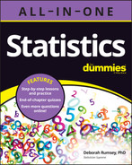
(say “mu” like in the word “music”); and its own standard deviation, denoted by the Greek letter ![]() (say “sigma”). But no matter what their means and standard deviations are, all normal distributions have the same basic bell shape. Figure 10-1 shows some examples of normal distributions.
(say “sigma”). But no matter what their means and standard deviations are, all normal distributions have the same basic bell shape. Figure 10-1 shows some examples of normal distributions.
Every normal distribution has certain properties. You use these properties to determine the relative standing of any particular result on the distribution, and to find probabilities. The properties of any normal distribution are as follows:
- Its shape is symmetric (that is, when you cut it in half, the two pieces are mirror images of each other).
- Its distribution has a bump in the middle, with tails going down and out to the left and right.
- The mean and the median are the same and lie directly in the middle of the distribution (due to symmetry).
- Its standard deviation measures the distance on the distribution from the mean to the inflection point (the place where the curve changes from an upside-down bowl shape to a right-side-up bowl shape).
- Because of its unique bell shape, probabilities for the normal distribution follow the Empirical Rule (full details in Chapter 5), which says the following:
- About 68 percent of its values lie within one standard deviation of the mean. To find this range, take the value of the standard deviation, then find the mean plus this amount, and the mean minus this amount.
- About 95 percent of its values lie within two standard deviations of the mean. (Here you take 2 times the standard deviation, then add it to and subtract it from the mean.)
- Almost all of its values (about 99.7 percent of them) lie within three standard deviations of the mean. (Take 3 times the standard deviation and add it to and subtract it from the mean.)
- Precise probabilities for all possible intervals of values on the normal distribution (not just for those within 1, 2, or 3 standard deviations from the mean) are found using a table with minimal (if any) calculations. (The next section gives you all the info on this table.)
Take a look at Figure 10-1. To compare and contrast the distributions shown in Figure 10-1a, b, and c, you first see they are all symmetric with the signature bell shape. The examples in Figure 10-1a and Figure 10-1b have the same standard deviation, but their means are different; Figure 10-1b is located 30 units to the right of Figure 10-1a because its mean is 120 compared to 90. Figures 10-1a and c have the same mean (90), but Figure 10-1a has more variability than Figure 10-1c due to its higher standard deviation (30 compared to 10). Because of the increased variability, the values in Figure 10-1a stretch from 0 to 180 (approximately), while the values in Figure 10-1c only go from 60 to 120.
Finally, Figures 10-1b and c have different means and different standard deviations entirely; Figure 10-1b has a higher mean, which shifts it to the right, and Figure 10-1c has a smaller standard deviation; its values are the most concentrated around the mean.
 Noting the mean and standard deviation is important so you can properly interpret numbers located on a particular normal distribution. For example, you can compare where the number 120 falls on each of the normal distributions in Figure 10-1. In Figure 10-1a, the number 120 is one standard deviation above the mean (because the standard deviation is 30, you get
 ![]() ). So on this first distribution, the number 120 is the upper value for the central range where about 68 percent of the data are located, according to the Empirical Rule (see Chapter 5).
). So on this first distribution, the number 120 is the upper value for the central range where about 68 percent of the data are located, according to the Empirical Rule (see Chapter 5).
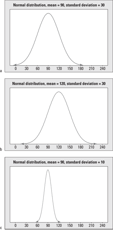
FIGURE 10-1: Three normal distributions, with means and standard deviations of a) 90 and 30; b) 120 and 30; and c) 90 and 10, respectively.
In Figure 10-1b, the number 120 lies directly on the mean, where the values are most concentrated. In Figure 10-1c, the number 120 is way out on the rightmost fringe, 3 standard deviations above the mean (because the standard deviation this time is 10, you get ![]() ). In Figure 10-1c, values beyond 120 are very unlikely to occur because they are beyond the central range where about 99.7 percent of the values should be, according to the Empirical Rule.
). In Figure 10-1c, values beyond 120 are very unlikely to occur because they are beyond the central range where about 99.7 percent of the values should be, according to the Empirical Rule.
 Q. Which of these two normal distributions has a larger variance?

A. The first distribution has a larger variance, because the data are more spread out from the center, and the tails take longer to go down and away.
1 What do you guess are the standard deviations of the two distributions in the previous example problem?
2 Draw a picture of a normal distribution with mean 70 and standard deviation 5.
3 Draw one picture containing two normal distributions. Give each a mean of 70, one a standard deviation of 5, and the other a standard deviation of 10. How do the distributions differ?
4 Suppose you have a normal distribution with mean 110 and standard deviation 15.
- About what percentage of the values lie between 110 and 125?
- About what percentage of the values lie between 95 and 140?
- About what percentage of the values lie between 80 and 95?
Meeting the Standard Normal (Z-) Distribution
One very special member of the normal distribution family is called the standard normal distribution, or Z-distribution. The Z-distribution is used to help find probabilities and percentiles for regular normal distributions (X). It serves as the standard by which all other normal distributions are measured.
Checking out Z
The Z-distribution is a normal distribution with mean zero and standard deviation 1; its graph is shown in Figure 10-2. Almost all (about 99.7 percent) of its values lie between –3 and 3 according to the Empirical Rule. Values on the Z-distribution are called z-values, z-scores, or standard scores. A z-value represents the number of standard deviations that a particular value lies above or below the mean. For example, ![]() on the Z-distribution represents a value that is 1 standard deviation above the mean. Similarly,
on the Z-distribution represents a value that is 1 standard deviation above the mean. Similarly, ![]() represents a value that is one standard deviation below the mean (indicated by the minus sign on the z-value). And a z-value of 0 is — you guessed it — right on the mean. All z-values are universally understood.
represents a value that is one standard deviation below the mean (indicated by the minus sign on the z-value). And a z-value of 0 is — you guessed it — right on the mean. All z-values are universally understood.

FIGURE 10-2: The Z-distribution has a mean of 0 and standard deviation of 1.
If you refer to Figure 10-1 and the discussion regarding where the number 120 lies on each normal distribution in the section, “Exploring the Basics of the Normal Distribution,” you can now calculate z-values to get a much clearer picture. In Figure 10-1a, the number 120 is located one standard deviation above the mean, so its z-value is 1. In Figure 10-1b, 120 is equal to the mean, so its z-value is 0. Figure 10-1c shows that 120 is 3 standard deviations above the mean, so its z-value is 3.
High standard scores (z-values) aren’t always the best. For example, if you’re measuring the amount of time needed to run around the block, a standard score of 2 is a bad thing because your time was two standard deviations above (more than) the overall average time. In this case, a standard score of –2 would be much better, indicating your time was two standard deviations below (less than) the overall average time.
Standardizing from X to Z
Probabilities for any continuous distribution are found by finding the area under a curve (if you’re into calculus, you know that means integration; if you’re not into calculus, don’t worry about it). Although the bell-shaped curve for the normal distribution looks easy to work with, calculating areas under its curve turns out to be a nightmare requiring high-level math procedures (believe me, I won’t be going there in this book!). Plus, every normal distribution is different, causing you to repeat this process over and over each time you have to find a new probability.
To help get over this obstacle, statisticians worked out all the math gymnastics for one particular normal distribution, made a table of its probabilities, and told the rest of us to knock ourselves out. Can you guess which normal distribution they chose to crank out the table for?
Yes, all the basic results you need to find probabilities for any normal distribution (X) can be boiled down into one table based on the standard normal (Z-) distribution. This table is called the Z-table and is found in the Appendix. Now all you need is one formula that transforms values from your normal distribution (X) to the Z-distribution; from there you can use the Z-table to find any probability you need.
Changing an x-value to a z-value is called standardizing. The so-called “z-formula” for standardizing an x-value to a z-value is:
You take your x-value, subtract the mean of X, and divide by the standard deviation of X. This gives you the corresponding standard score (z-value or z-score).
Standardizing is just like changing units (for example, from Fahrenheit to Celsius). It doesn’t affect probabilities for X; that’s why you can use the Z-table to find them!
 You can standardize an x-value from any distribution (not just the normal) using the z-formula. Similarly, not all standard scores come from a normal distribution.
Because you subtract the mean from your x-values and divide everything by the standard deviation when you standardize, you are literally taking the mean and standard deviation of X out of the equation. This is what allows you to compare everything on the scale from –3 to 3 (the Z-distribution), where negative values indicate being below the mean, positive values indicate being above the mean, and a value of 0 indicates you’re right on the mean.
Standardizing also allows you to compare numbers from different distributions. For example, suppose Bob scores 80 on both his math exam (which has a mean of 70 and a standard deviation of 10) and his English exam (which has a mean of 85 and a standard deviation of 5). On which exam did Bob do better, in terms of his relative standing in the class?
Bob’s math exam score of 80 standardizes to a z-value of ![]() . That tells you his math score is one standard deviation above the class average. His English exam score of 80 standardizes to a z-value of
. That tells you his math score is one standard deviation above the class average. His English exam score of 80 standardizes to a z-value of ![]() , putting him one standard deviation below the class average. Even though Bob scored 80 on both exams, he actually did better on the math exam than the English exam, relatively speaking.
, putting him one standard deviation below the class average. Even though Bob scored 80 on both exams, he actually did better on the math exam than the English exam, relatively speaking.
To interpret a standard score, you don’t need to know the original score, the mean, or the standard deviation. The standard score gives you the relative standing of a value, which in most cases is what matters most. In fact, on most national achievement tests, they won’t even tell you what the mean and standard deviation were when they report your results; they just tell you where you stand on the distribution by giving you your z-score.
Finding probabilities for Z with the Z-table
A full set of less-than probabilities for a wide range of z-values is in the Z-table (Table A-1 in the Appendix). To use the Z-table to find probabilities for the standard normal (Z-) distribution, do the following:
- Go to the row that represents the first digit of your z-value and the first digit after the decimal point.
- Go to the column that represents the second digit after the decimal point of your z-value.
Intersect the row and column.
This result represents
 , the probability that the random variable Z is less than or equal to the number z (also known as the percentage of z-values that are less than yours).
For example, suppose you want to find ![]() . Using the Z-table, find the row for 2.1 and the column for 0.03. Intersect that row and column to find the probability: 0.9834. You find that
. Using the Z-table, find the row for 2.1 and the column for 0.03. Intersect that row and column to find the probability: 0.9834. You find that ![]() .
.
Suppose you want to look for ![]() . You find the row for –2.1 and the column for 0.03. Intersect the row and column and you find 0.0166; that means
. You find the row for –2.1 and the column for 0.03. Intersect the row and column and you find 0.0166; that means ![]() equals 0.0166. (This happens to be one minus the probability that Z is less than 2.13 because
equals 0.0166. (This happens to be one minus the probability that Z is less than 2.13 because ![]() equals 0.9834. That’s true because the normal distribution is symmetric; more on that in the following section.)
equals 0.9834. That’s true because the normal distribution is symmetric; more on that in the following section.)
Q. Suppose you play a round of golf and want to compare your score to the other members of your club population. You find that your score is below the mean.
- What does this tell you about your standard score?
- Is this a good thing or a bad thing?
A. To interpret the standard score, the sign is the first part to look at.
- Falling below the mean indicates a negative standard score.
- Often, being below the mean is a bad thing, but in golf you have an advantage because golf scores measure the number of swings you need to get around the course, and you want to have a low golf score. So being below the mean in this case is a good thing.
5 Exam scores have a normal distribution with a mean of 70 and a standard deviation of 10. Bob’s score is 80. Find and interpret his standard score.
6 Bob scores 80 on both his math exam (which has a mean of 70 and a standard deviation of 10) and his English exam (which has a mean of 85 and a standard deviation of 5). Find and interpret Bob’s z-scores on both exams to let him know which exam (if either) he did better on. Don’t, however, let his parents know; let them think he’s just as good at both subjects.
7 Sue’s math class’s exam has a mean of 70 with a standard deviation of 5. Her standard score is –2. What’s her original exam score?
8 Suppose your score on an exam is directly at the mean. What’s your standard score?
9 Suppose the weights of cereal boxes have a normal distribution with a mean of 20 ounces and a standard deviation of half an ounce. A box that has a standard score of zero weighs how much?
10 Suppose you want to put fat Fido on a weight-loss program. Before the program, his weight had a standard score of 2 compared to dogs of his breed and age, and after the program, his weight has a standard score of –2. His weight before the program was 150 pounds, and the standard deviation for the breed is 5 pounds.
- What’s the mean weight for Fido’s breed and age?
- What’s his weight after the weight-loss program?
Finding Probabilities for a Normal Distribution
Here are the steps for finding a probability when X has any normal distribution:
- Draw a picture of the distribution.
- Translate the problem into one of the following:
 , or
, or  . Shade in the area on your picture.
 - Standardize a (and/or b) to a z-score using the z-formula:

Look up the z-score on the Z-table (Table A-1 in the Appendix) and find its corresponding probability.
(See the section, “Standardizing from X to Z,” for more on the Z-table).
5a. If you need a “less-than” probability — that is, ![]() — you’re done.
— you’re done.
5b. If you want a “greater-than” probability — that is, ![]() — take one minus the result from Step 4.
— take one minus the result from Step 4.
5c. If you need a “between-two-values” probability — that is, ![]() — do Steps 1–4 for b (the larger of the two values) and again for a (the smaller of the two values), and subtract the results.
— do Steps 1–4 for b (the larger of the two values) and again for a (the smaller of the two values), and subtract the results.
The probability that X is equal to any single value is 0 for any continuous random variable (like the normal). That’s because continuous random variables consider probability as being area under the curve, and there’s no area under a curve at one single point. So, ![]() , and also
, and also ![]() . This isn’t true of discrete random variables.
. This isn’t true of discrete random variables.
Suppose, for example, that you enter a fishing contest. The contest takes place in a pond where the fish lengths have a normal distribution with mean ![]() inches and standard deviation
inches and standard deviation ![]() inches.
inches.
- Problem 1: What’s the chance of catching a small fish — say, less than or equal to 8 inches?
- Problem 2: Suppose a prize is offered for any fish over 24 inches. What’s the chance of winning a prize?
- Problem 3: What’s the chance of catching a fish between 16 and 24 inches?
To solve these problems using the steps that I just listed, first draw a picture of the normal distribution at hand. Figure 10-3 shows a picture of X’s distribution for fish lengths. You can see where the numbers of interest (8, 16, and 24) fall.
Next, translate each problem into probability notation. Problem 1 is really asking you to find ![]() . For Problem 2, you want
. For Problem 2, you want ![]() . And Problem 3 is looking for
. And Problem 3 is looking for ![]() .
.
FIGURE 10-3: The distribution of fish lengths in a pond (X).
Step 3 says to change the x-values to z-values using the z-formula:
For Problem 1 of the fish example, you have the following:
Similarly for Problem 2, ![]() becomes
becomes
And Problem 3 translates from ![]() to
to
Figure 10-4 shows a comparison of the X-distribution and Z-distribution for the values ![]() , and 24, which standardize to
, and 24, which standardize to ![]() , and 2, respectively.
, and 2, respectively.
Now that you have changed x-values to z-values, you move to Step 4 and find (or calculate) probabilities for those z-values using the Z-table (in the Appendix). In Problem 1 of the fish example, you want ![]() ; go to the Z-table and look at the row for –2.0 and the column for 0.00, intersect them, and you find 0.0228 — according to Step 5a, you’re done. The chance of a fish being less than or equal to 8 inches is equal to 0.0228.
; go to the Z-table and look at the row for –2.0 and the column for 0.00, intersect them, and you find 0.0228 — according to Step 5a, you’re done. The chance of a fish being less than or equal to 8 inches is equal to 0.0228.
For Problem 2, find ![]() . Because it’s a “greater-than” problem, this calls for Step 5b. To be able to use the Z-table, you need to rewrite this in terms of a “less-than” statement. Because the entire probability for the Z-distribution equals 1, you know
. Because it’s a “greater-than” problem, this calls for Step 5b. To be able to use the Z-table, you need to rewrite this in terms of a “less-than” statement. Because the entire probability for the Z-distribution equals 1, you know ![]() (using the Z-table). So, the chance that a fish is greater than 24 inches is also 0.0228. (Note: The answers to Problems 1 and 2 are the same because the Z-distribution is symmetric; refer to Figure 10-3.)
(using the Z-table). So, the chance that a fish is greater than 24 inches is also 0.0228. (Note: The answers to Problems 1 and 2 are the same because the Z-distribution is symmetric; refer to Figure 10-3.)
In Problem 3, you find ![]() ; this requires Step 5c. First, find
; this requires Step 5c. First, find ![]() , which is 0.9772 from the Z-table. Then find
, which is 0.9772 from the Z-table. Then find ![]() , which is 0.5000 from the Z-table. Subtract them to get
, which is 0.5000 from the Z-table. Subtract them to get ![]() . The chance of a fish being between 16 and 24 inches is 0.4772.
. The chance of a fish being between 16 and 24 inches is 0.4772.

FIGURE 10-4: Standardizing numbers from a normal distribution (X) to numbers on the Z-distribution.
The Z-table does not list every possible value of Z; it just carries them out to two digits after the decimal point. Use the one closest to the one you need. And just like in an airplane where the closest exit may be behind you, the closest z-value may be the one that is lower than the one you need.
Q. The weights of single-dip ice cream cones at Bob’s ice cream parlor have a normal distribution with a mean of 8 ounces and a standard deviation of one-half ounce (0.5 ounce). What’s the chance that an ice cream cone weighs between 7 and 9 ounces?
A. In this case, you want ![]() , the area between two values. Convert both of the values to z-scores, find their probabilities on the Z-table (see Table A-1), and subtract them taking the largest one minus the smallest one. Nine ounces becomes
, the area between two values. Convert both of the values to z-scores, find their probabilities on the Z-table (see Table A-1), and subtract them taking the largest one minus the smallest one. Nine ounces becomes ![]() . The corresponding probability is
. The corresponding probability is ![]() . Seven ounces becomes
. Seven ounces becomes ![]() , which has a corresponding probability of
, which has a corresponding probability of ![]() . Subtracting these probabilities gives you the area between them:
. Subtracting these probabilities gives you the area between them: ![]() . Note that 0.9544 is equivalent to
. Note that 0.9544 is equivalent to ![]() .
.
11 Bob’s commuting times to work have a normal distribution with a mean of 45 minutes and a standard deviation of 10 minutes. How often does Bob get to work in 30 to 45 minutes?
12 The times taken to complete a statistics exam have a normal distribution with a mean of 40 minutes and a standard deviation of 6 minutes. What’s the chance of Deshawn completing the exam in 30 to 35 minutes?
13 Times until service at a restaurant have a normal distribution with a mean of 10 minutes and a standard deviation of 3 minutes. What’s the chance of it taking longer than 15 minutes to get service?
14 At the same restaurant as in the preceding question with the same normal distribution, what’s the chance of it taking no more than 15 minutes to get service?
15 Clint, obviously not in college, sleeps an average of 8 hours per night with a standard deviation of 15 minutes. What’s the chance of him sleeping between 7.5 and 8.5 hours on any given night?
16 One state’s annual rainfall has a normal distribution with a mean of 100 inches and a standard deviation of 25 inches. Suppose corn grows best when the annual rainfall is between 100 and 140 inches. What’s the chance of achieving this amount of rainfall?
Knowing Where You Stand with Percentiles
Percentiles are a way to measure where you stand in a data set. Do you remember the last time you took a standardized test? Not only did the testing company give you your raw score, but they probably also gave you a percentile. If you come in at the 90th percentile, for example, 90 percent of the test scores of all students are the same as or below yours (and 10 percent are above yours). Pediatricians track the growth of newborn babies by the percentile of their length, weight, and head circumference. In general, being at the kth percentile means k percent of the data lie at or below that point and ![]() percent lie above it.
percent lie above it.
You saw how to calculate the 25th and 75th percentiles for getting a five-number summary in Chapter 5. To calculate a percentile when the data has a normal distribution is essentially like finding a probability for a given value:
- Convert the original score to a standard score by taking the original score minus the mean and dividing by the standard deviation (in other words, use the z-formula).
- Use the Z-table to find the corresponding percentile for the standard score.
The percentage is the probability you find in the Z-table. The percentile is the value of X (a test score, your height, and so forth) with a specific percentage of values less than its value.
Q. Weights for single-dip ice cream cones at Adrian’s have a normal distribution with a mean of 8 ounces and a standard deviation of one-quarter ounce. Suppose your ice cream cone weighs 8.5 ounces. What percentage of cones is smaller than yours?
A. Your cone weighs 8.5 ounces, and you want the corresponding percentile. Before you can use the Z-table to find that percentile, you need to standardize the 8.5 — in other words, run it through the z-formula. This gives you ![]() , so the z-score for your ice cream cone is 2. Now you use the Z-table to find that a z-value of 2.00 corresponds with 0.9772, which equals 97.72 percent. Your ice cream cone is at the 97.72th percentile, and 97.72 percent of the other single-dip cones at Adrian’s are smaller than yours. Lucky you!
, so the z-score for your ice cream cone is 2. Now you use the Z-table to find that a z-value of 2.00 corresponds with 0.9772, which equals 97.72 percent. Your ice cream cone is at the 97.72th percentile, and 97.72 percent of the other single-dip cones at Adrian’s are smaller than yours. Lucky you!
17 Bob’s commuting times to work have a normal distribution with a mean of 45 minutes and a standard deviation of 10 minutes.
- What percentile does Bob’s commute time represent if he gets to work in 30 minutes or less?
- Bob’s workday starts at 9 a.m. If he leaves at 8 a.m., how often is he late?
18 Suppose your exam score has a standard score of 0.90. Does this mean that 90 percent of the other exam scores are lower than yours?
19 If a baby’s weight is at the median, what’s their percentile?
20 Suppose you know that Layton’s test score is above the mean in a normal distribution of scores, but he doesn’t remember by how much. At least how many students must score lower than Layton?
Finding X When You Know the Percent
Another popular normal distribution problem involves finding percentiles for X (see Chapter 5 for a detailed rundown on percentiles). That is, you are given the percentage or probability of being at or below a certain x-value, and you have to find the x-value that corresponds to it. For example, if you know that the people whose golf scores were in the lowest 10 percent got to go to the tournament, you may wonder what the cutoff score was; that score would represent the 10th percentile.
 A percentile isn’t a percent. A percent is a number between 0 and 100; a percentile is a value of X (a height, an IQ, a test score, and so on).
Figuring out a percentile for a normal distribution
Certain percentiles are so popular that they have their own names and their own notation. The three “named” percentiles are ![]() — the first quartile, or the 25th percentile;
— the first quartile, or the 25th percentile; ![]() — the second quartile (also known as the median or the 50th percentile); and
— the second quartile (also known as the median or the 50th percentile); and ![]() — the third quartile or the 75th percentile. (See Chapter 5 for more information on quartiles.)
— the third quartile or the 75th percentile. (See Chapter 5 for more information on quartiles.)
Here are the steps for finding any percentile for a normal distribution X:
1a. If you’re given the probability (percent) less than x and you need to find x, you translate this as follows: Find a where ![]() (and p is the given probability). That is, find the pth percentile for X. Go to Step 2.
(and p is the given probability). That is, find the pth percentile for X. Go to Step 2.
1b. If you’re given the probability (percent) greater than x and you need to find x, you translate this as follows: Find b where ![]() (and p is given). Rewrite this as a percentile (less-than) problem: Find b where
(and p is given). Rewrite this as a percentile (less-than) problem: Find b where ![]() . This means find the (1 – p)th percentile for X.
. This means find the (1 – p)th percentile for X.
- Find the corresponding percentile for Z by looking in the body of the Z-table (Table A-1 in the Appendix) and finding the probability that is closest to p (from Step 1a) or 1 – p (from Step 1b). Find the row and column this probability is in (using the table backwards). This is the desired z-value.
Change the z-value back into an x-value (original units) by using
 . You’ve (finally!) found the desired percentile for X.
The formula in this step is just a rewriting of the z-formula,
 , so it’s solved for x.
Doing a low percentile problem
Look at the fish example used previously in “Finding Probabilities for a Normal Distribution,” where the lengths (X) of fish in a pond have a normal distribution with a mean of 16 inches and a standard deviation of 4 inches. Suppose you want to know what length marks the bottom 10 percent of all the fish lengths in the pond. What percentile are you looking for?
Being at the bottom 10 percent means you have a “less-than” probability that’s equal to 10 percent, and you are at the 10th percentile.
Now go to Step 1a in the preceding section and translate the problem. In this case, because you’re dealing with a “less-than” situation, you want to find x such that ![]() . This represents the 10th percentile for X. Figure 10-5 shows a picture of this situation.
. This represents the 10th percentile for X. Figure 10-5 shows a picture of this situation.

FIGURE 10-5: Bottom 10 percent of fish in the pond, according to length.
Now go to Step 2, which says to find the 10th percentile for Z. Looking in the body of the Z-table (in the Appendix), the probability closest to 0.10 is 0.1003, which falls in the row for ![]() and the column for 0.08. That means the 10th percentile for Z is –1.28; so a fish whose length is 1.28 standard deviations below the mean marks the bottom 10 percent of all fish lengths in the pond.
and the column for 0.08. That means the 10th percentile for Z is –1.28; so a fish whose length is 1.28 standard deviations below the mean marks the bottom 10 percent of all fish lengths in the pond.
But exactly how long is that fish, in inches? In Step 3, you change the z-value back to an x-value (fish length in inches) using the z-formula solved for x; you get ![]() inches. So 10.88 inches marks the lowest 10 percent of fish lengths. Ten percent of the fish are as short as or shorter than that.
inches. So 10.88 inches marks the lowest 10 percent of fish lengths. Ten percent of the fish are as short as or shorter than that.
Working with a higher percentile
Now suppose you want to find the length that marks the top 25 percent of all the fish in the pond. This problem calls for Step 1b (in the section, “Finding a percentile for a normal distribution”) because being in the top part of the distribution means you’re dealing with a greater-than probability. The number you are looking for is somewhere in the right tail (upper area) of the X-distribution, with ![]() of the probability to its right and
of the probability to its right and ![]() to its left. Thinking in terms of the Z-table and how it only uses less-than probabilities, you need to find the 75th percentile for Z, and then change it to an x-value.
to its left. Thinking in terms of the Z-table and how it only uses less-than probabilities, you need to find the 75th percentile for Z, and then change it to an x-value.
Step 2: The 75th percentile of Z is the z-value where ![]() . Using the Z-table (in the Appendix), you find the probability closest to 0.7500 is 0.7486, and its corresponding z-value is in the row for 0.6 and the column for 0.07. Put these together and you get a z-value of 0.67. This is the 75th percentile for Z. In Step 3, change the z-value back to an x-value (length in inches) using the z-formula solved for x to get
. Using the Z-table (in the Appendix), you find the probability closest to 0.7500 is 0.7486, and its corresponding z-value is in the row for 0.6 and the column for 0.07. Put these together and you get a z-value of 0.67. This is the 75th percentile for Z. In Step 3, change the z-value back to an x-value (length in inches) using the z-formula solved for x to get ![]() inches. So, 75 percent of the fish are at least as short as 18.68 inches. And to answer the original question, the top 25 percent of the fish in the pond are longer than 18.68 inches.
inches. So, 75 percent of the fish are at least as short as 18.68 inches. And to answer the original question, the top 25 percent of the fish in the pond are longer than 18.68 inches.
Translating tricky wording in percentile problems
Some percentile problems are especially challenging to translate. For example, suppose the amount of time for a racehorse to run around a track in a qualifying round has a normal distribution with a mean of 120 seconds and a standard deviation of 5 seconds. The best 10 percent of the times qualify; the rest don’t. What’s the cutoff time for qualifying?
Because “best times” means “lowest times” in this case, the percentage of times that lie below the cutoff must be 10, and the percentage above the cutoff must be 90. (It’s an easy mistake to think it’s the other way around.) The percentile of interest is therefore the 10th, which is down on the left tail of the distribution. You now work this problem the same way I worked the earlier problem regarding fish lengths (see the section, “Finding Probabilities for a Normal Distribution”). The standard score for the 10th percentile is ![]() looking at the Z-table (in the Appendix). Converting back to original units, you get
looking at the Z-table (in the Appendix). Converting back to original units, you get ![]() seconds. So the cutoff time needed for a racehorse to qualify (that is, to be among the fastest 10 percent) is 113.6 seconds. (Notice this number is less than the average time of 120 seconds, which makes sense; a negative z-value is what makes this happen.)
seconds. So the cutoff time needed for a racehorse to qualify (that is, to be among the fastest 10 percent) is 113.6 seconds. (Notice this number is less than the average time of 120 seconds, which makes sense; a negative z-value is what makes this happen.)
The 50th percentile for the normal distribution is the mean (because of symmetry) and its z-score is zero. Smaller percentiles, like the 10th, lie below the mean and have negative z-scores. Larger percentiles, like the 75th, lie above the mean and have positive z-scores.
Here’s another style of wording that has a bit of a twist: Suppose times to complete a statistics exam have a normal distribution with a mean of 40 minutes and a standard deviation of 6 minutes. Deshawn’s time comes in at the 90th percentile. What percentage of the students are still working on their exams when Deshawn leaves? Because Deshawn is at the 90th percentile, 90 percent of the students have exam times lower than hers. That means 90 percent of the students left before Deshawn, so ![]() percent of the students are still working when Deshawn leaves.
percent of the students are still working when Deshawn leaves.
To be able to decipher the language used to imply a percentile problem, look for clues like the bottom 10 percent (also known as the 10th percentile) and the top 10 percent (also known as the 90th percentile). For the best 10 percent, you must determine whether low or high numbers qualify as “best.”
Q. Racehorses race around the track in a qualifying round according to a normal distribution with a mean of 120 seconds and a standard deviation of 5 seconds. Now suppose the bottom 10 percent of the times get eliminated from the next race. What’s the cutoff time for being eliminated?
A. You may think you need to find the 10th percentile, but no. The smaller values for times don’t get eliminated. The largest 10 percent of the times do get eliminated, so in terms of data on a normal distribution, you know that the percentile of interest is the 90th. Remember that the percentage of times below the cutoff is 90, and the percentage above the cutoff is 10 (that’s how percentiles work). The standard score for the 90th percentile is found by seeking out 0.90 in the body of the Z-table. The closest value to this is 0.8997, which matches up with a z-value of +1.28. Converting this back to the original units, you get ![]() . So the cutoff time for being eliminated from the next race is 126.4 seconds.
. So the cutoff time for being eliminated from the next race is 126.4 seconds.
21 Weights have a normal distribution with a mean of 100 and a standard deviation of 10. What weight has 60 percent of the values lying below it?
22 Jimmy walks a mile, and his previous times have a normal distribution with a mean of 8 minutes and a standard deviation of 1 minute. What time does he have to make to get into his own top 10 percent of his fastest times?
23 The times it takes to complete a statistics exam have a normal distribution with a mean of 40 minutes and a standard deviation of 6 minutes. Deshawn’s time falls at the 42nd percentile. How long does Deshawn take to finish her exam?
24 Exam scores for a particular test have a normal distribution with a mean of 75 and a standard deviation of 5. The instructor wants to give the top 20 percent of the scores an A. What’s the cutoff for an A?
25 Service call times for one company have a normal distribution with a mean of 10 minutes and a standard deviation of 3 minutes. Researchers study the longest 25 percent of the calls to make improvements. How long do the longest 25 percent last?
26 Statcars are new vehicles whose mileage has a normal distribution with a mean of 75 miles per gallon. Twenty percent of the vehicles get more than 100 miles per gallon. What’s the standard deviation?
Normal Approximation to the Binomial
Suppose you flip a fair coin 100 times and you let X equal the number of heads. What’s the probability that X is greater than 60? In Chapter 9, you solve problems like this (involving fewer flips) using the binomial distribution. For binomial problems where n (the number of trials) is small, you can use the direct formula (found in Chapter 9), the binomial table (found in the Appendix), or technology if it is available (such as a graphing calculator or Microsoft Excel).
However, if n is large, the calculations get unwieldy and the binomial table runs out of numbers. If there’s no technology available (like when taking an exam), what can you do to find a binomial probability? Turns out, if n is large enough, you can use the normal distribution to find a very close approximate answer with a lot less work.
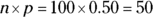
But what do I mean by n being “large enough”? To determine whether n is large enough to use what statisticians call the normal approximation to the binomial, both of the following conditions must hold:
 (at least 10), where p is the probability of success
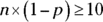 (at least 10), where
  is the probability of failure
To find the normal approximation to the binomial distribution when n is large, use the following steps:
Verify whether n is large enough to use the normal approximation by checking the two appropriate conditions.
For the coin-flipping question, the conditions are met because
 , and
, and  , both of which are at least 10. So go ahead with the normal approximation.
Translate the problem into a probability statement about X.
For the coin-flipping example, you need to find
 .
.- Standardize the x-value to a z-value, using the z-formula:

For the mean of the normal distribution, use
 (the mean of the binomial), and for the standard deviation
  , use
, use  (the standard deviation of the binomial; see Chapter 9).
For the coin-flipping example,
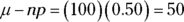 and
and  . Now put these values into the z-formula to get
 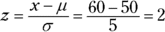 . To solve the problem, you need to find
  . On an exam, you won’t see
  and
and  in the problem when you have a binomial distribution. However, you know the formulas that allow you to calculate both of them using n and p (values which will be given in the problem). Just remember you have to do that extra step to calculate the
  and
and  needed for the z-formula.
 Proceed as you usually would for any normal distribution. That is, do Steps 4 and 5 described in the earlier section, “Finding Probabilities for a Normal Distribution.”
Continuing the example,
 from the Z-table (found in the Appendix). So the chance of getting more than 60 heads in 100 flips of a coin is only about 2.28 percent. (I wouldn’t bet on it.)
When using the normal approximation to find a binomial probability, your answer is an approximation (not exact) — be sure to state that. Also show that you checked both necessary conditions for using the normal approximation.
Q. Suppose that 60 percent of the crowd at a music festival is female. If 40 people will be randomly selected to win an attendance prize, what is the chance that at least 20 of the winners will be female?
A. You have a fixed number of trials ![]() with a defined probability of success
with a defined probability of success ![]() of a selected person being female. Hey, this is talking about a binomial random variable! Unfortunately, Table A-3 only goes up to
of a selected person being female. Hey, this is talking about a binomial random variable! Unfortunately, Table A-3 only goes up to ![]() . Instead, check to see whether you can use the normal approximation to the binomial. You find that
. Instead, check to see whether you can use the normal approximation to the binomial. You find that ![]() and
and ![]() are both greater than 10, so you can go ahead with the approximation.
are both greater than 10, so you can go ahead with the approximation.
For Step 2, identify the probability by writing it as ![]() . Next, you need to standardize the x-value of 20 into its proper z-value. Remember to first find the mean
. Next, you need to standardize the x-value of 20 into its proper z-value. Remember to first find the mean ![]() and the standard deviation
and the standard deviation ![]() . Putting these into the z-formula, you get
. Putting these into the z-formula, you get ![]() . To solve the problem, you need to find
. To solve the problem, you need to find ![]() . From the Z-table, you can look up that
. From the Z-table, you can look up that ![]() , which means that
, which means that ![]() . So the chance that at least 20 of the 40 winners will be female is approximately 90.15 percent.
. So the chance that at least 20 of the 40 winners will be female is approximately 90.15 percent.
27 At a certain major airport, 15 percent of all travelers are headed to an international destination. If you ask 500 random people where they’re headed, what’s the probability that less than 80 of them are flying internationally?
28 You are in charge of one of the rides at StatWorld, the greatest amusement park on earth! Historically, 95 percent of park guests who get on your ride are children. Your manager wants to know the chance that less than 140 of the next 150 riders will be children. Can you use a normal approximation to the binomial to answer the manager’s question?
29 As a basketball player, you successfully make 50 percent of your shots. (Wow! You should be in the NBA.) Assuming that the likelihood of you scoring a basket is independent from one shot to the next, you’re interested in guessing how many of the next 20 shots you will make.
- Calculate the probability that you will make at least 10 of your next 20 shots using the binomial table.
- Calculate the probability that you will make at least 10 of your next 20 shots using a normal approximation.
- How do the two calculations compare?
Practice Questions Answers and Explanations
1 In the first normal distribution, most of the data falls between 10 and 70, each within 3 times 10 units of the mean (40), so you can assume the standard deviation is around 10. You can also see that the saddle point (the place where the picture changes from an upside-down bowl shape to a right-side-up bowl shape) occurs about 10 units away from the mean of 40, which means the standard deviation is around 10. In the second normal distribution, the saddle point occurs about 5 units from the mean, so the standard deviation is at about 5. Notice also that most all the data lies within 15 units of the mean, which is 3 standard deviations.
2 See the following figure. Check that you have saddle points at 65 and 75.

3 See the following figure. A graph with a standard deviation of 5 is taller and thinner than a graph whose standard deviation is 10. The normal distribution with a standard deviation of 10 is more spread out and flatter looking than the normal distribution with a standard deviation of 5, which looks more squeezed together close to the mean (which it is).

A normal distribution that looks flatter actually has more variability than one that goes from low to high to low as you look from left to right, because you measure variability by how far away the values are from the middle; more data close to the middle means low variability, and more data farther away means less variability. This characteristic differs from what you see on a graph that shows data over time (time series or line graphs). On the time graphs, a flat line means no change over time, and going from low to high to low means great variability.
4 A picture is worth a thousand points here (along with the Empirical Rule). See the following figure.

- For the two values 110 and 125, 125 is one standard deviation above the mean, and about 68 percent of the values lie within one standard deviation of the mean (on both sides of it). So, the percentage of values between 110 and 125 is half of 68 percent, which is 34 percent. The following figure illustrates this point.
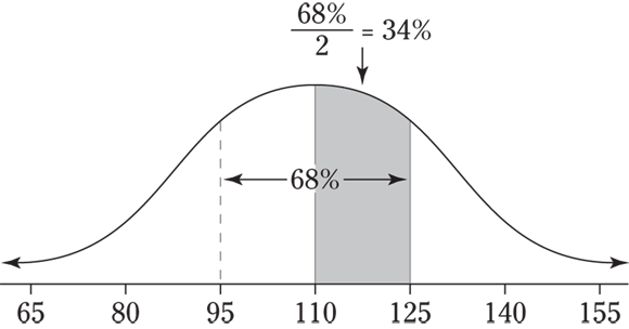
- For the two values 95 and 140, 95 is one standard deviation below the mean (110), so that distance covers half of the 68 percent again, or 34 percent. To get from 110 to 140, you need to go two standard deviations above the mean. Because about 95 percent of the data lie within two standard deviations of the mean (on both sides of it), from 110 to 140 covers about half of the 95 percent, which is 47.5 percent. Add the 34 and the 47.5 to get 81.5 percent for your approximate answer. See the following figure for an illustration.
- For the two values 80 and 95, 80 is two standard deviations below the mean of 110, which represents
 or 47.5 percent of the data. And 95 is one standard deviation below 110, which represents
  or 34 percent of the data. You want the area between these two values, so subtract the percentages:
 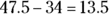 percent. See the following figure for a visual.
 When using the Empirical Rule to find the percentage between two values, you may have to use a different approach, depending on whether both values are on the same side of the mean or one is above the mean and one below the mean. First, find the percentages that lie between the mean and each value separately. If the values fall on different sides of the mean, add the percentages together. When they appear on the same side of the mean, subtract their percentages (largest minus smallest, so the answer isn’t negative). Or, better yet, draw a picture to see what you need to do.
5 The following figure shows a picture of this distribution. Take ![]() and divide by 10 to get 1. Bob’s score is one standard deviation above the mean. You can see this on a picture as well, because Bob’s score falls one “tick mark” above the mean on the picture of the original normal distribution.
and divide by 10 to get 1. Bob’s score is one standard deviation above the mean. You can see this on a picture as well, because Bob’s score falls one “tick mark” above the mean on the picture of the original normal distribution.

6 The 80 Bob scores on his math exam converts to a standard score of 1 (see the preceding answer). The 80 Bob scores on his English exam converts to a standard score of ![]() . His score on the English exam is one standard deviation below the mean, so his math score is better.
. His score on the English exam is one standard deviation below the mean, so his math score is better.
Your actual scores don’t matter; what matters is how you compare to the mean, in terms of number of standard deviations.
7 Here you can use the same formula, ![]() , but you need to plug in different values. You know the mean is 70 and the standard deviation is 5. You know
, but you need to plug in different values. You know the mean is 70 and the standard deviation is 5. You know ![]() , but you don’t know x, the original score. So what you have looks like
, but you don’t know x, the original score. So what you have looks like ![]() . Solving for x, you get
. Solving for x, you get ![]() , so
, so ![]() , or
, or ![]() . The answer makes sense because each standard deviation is worth five, and you start at 70 and go down two of these standard deviations:
. The answer makes sense because each standard deviation is worth five, and you start at 70 and go down two of these standard deviations: ![]() . So Sue scored a 60 on the test.
. So Sue scored a 60 on the test.
8 A standard score of zero means your original score is the mean itself, because the standard score is the number of standard deviations above or below the mean. When your score is on the mean, you don’t move away from it at all. Also, in the z-formula, after you take the value (which is at the mean) and subtract the mean, you get zero in the numerator, so the answer is zero.
9 Exactly 20 ounces, because a standard score of zero means the observation is right on the mean.
10 This problem is much easier to calculate if you first draw a picture of what you know and work from there.
- The following figure shows a picture of the situation before and after Fido’s weight-loss program. You know that 150 has a z-score of 2 and the standard deviation is 5, so you have
 . And solving for the mean
  , you calculate
  . The mean weight for his breed and age group is 140 pounds.

- A z-score of –2 corresponds to a weight 2 standard deviations below the mean of 150, which brings you down to
 . Fido weighs 130 pounds after the program.
For any problem involving a normal distribution, drawing a picture is the key to success.
. Fido weighs 130 pounds after the program.
For any problem involving a normal distribution, drawing a picture is the key to success.
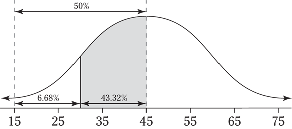
11 The following figure shows a picture of the situation. You want ![]() , the probability that X is between 30 and 45, where X is the commuting time. Converting the 30 to a standard score with the z-formula, you get
, the probability that X is between 30 and 45, where X is the commuting time. Converting the 30 to a standard score with the z-formula, you get ![]() . The value 45 converts to
. The value 45 converts to ![]() because it’s right at the mean. (Or, note that
because it’s right at the mean. (Or, note that ![]() , and 0 divided by 10 is still 0.) Because you have to find the probability of being between two numbers, look up each of the probabilities associated with their standard scores on the Z-table (see Table A-1) and subtract their values (largest minus smallest, to avoid a negative answer). Using the Z-table,
, and 0 divided by 10 is still 0.) Because you have to find the probability of being between two numbers, look up each of the probabilities associated with their standard scores on the Z-table (see Table A-1) and subtract their values (largest minus smallest, to avoid a negative answer). Using the Z-table, ![]() and
and ![]() . Subtracting those values gives you
. Subtracting those values gives you ![]() , which is equivalent to 43.32 percent.
, which is equivalent to 43.32 percent.
The reason you subtract the two probabilities when finding the chance of being between two numbers is because the probability includes all the area less than or equal to a certain value. You want the probability of being less than or equal to the larger number, but you don’t want the probability of being less than or equal to the smaller number. Subtracting the percentiles allows you to keep the part you want and throw away the part you don’t want.
12 The following figure shows a picture of this situation. You want the probability that X (exam time) is between two values, 30 and 35, on the normal distribution. First, convert each of the values to standard scores, using the z-formula. The 30 converts to ![]() , and
, and ![]() . The 35 converts to
. The 35 converts to ![]() , and
, and ![]() . To get the probability, or area, between the two values, subtract each of their percentiles — the larger one minus the smaller one — to get
. To get the probability, or area, between the two values, subtract each of their percentiles — the larger one minus the smaller one — to get ![]() , which is equivalent to 15.58 percent.
, which is equivalent to 15.58 percent.

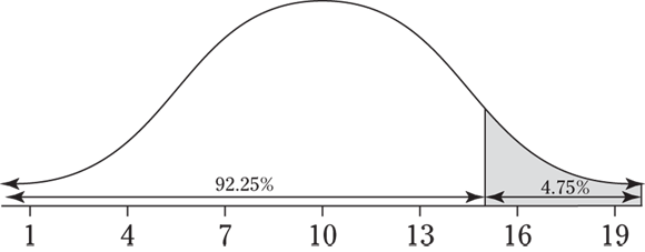
13 You are looking for the probability that X (service time) is more than 15 minutes (see the following figure). In this case, you convert the value to a standard score, find its probability, and take 100 minus that probability because you want the percentage that falls above it. Substituting the values, you have ![]() , and using Table A-1, you find that
, and using Table A-1, you find that ![]() . The probability you want is
. The probability you want is ![]() , which is equivalent to 4.75 percent.
, which is equivalent to 4.75 percent.
14 This problem is the exact opposite (or complement) of the preceding problem. Here you want the probability that X is no more than 15, which means the probability X is less than or equal to 15, ![]() . If 4.75 percent (.0475) is the probability of being more than 15 in the last problem, then the probability of being less than or equal to 15 is
. If 4.75 percent (.0475) is the probability of being more than 15 in the last problem, then the probability of being less than or equal to 15 is ![]() , which is 0.9525 or 95.25 percent.
, which is 0.9525 or 95.25 percent.
The chance of X being exactly equal to a certain value on a normal distribution is zero, so it doesn’t matter whether you take the probability that X is less than 15, ![]() , or the probability that X is less than or equal to 15,
, or the probability that X is less than or equal to 15, ![]() . You get the same answer, because the probability that X equals the one specific value of exactly 15 is zero.
. You get the same answer, because the probability that X equals the one specific value of exactly 15 is zero.
15 For this problem, you need to convert 7.5 and 8.5 to standard scores, look up their percentiles on the Z-table (Table A-1), and subtract them by taking the largest one minus the smallest one. Note that the standard deviation given in the problem is stated in minutes. Convert this to hours first by taking ![]() . For this problem, 7.5 converts to a standard score of
. For this problem, 7.5 converts to a standard score of ![]() . And 8.5 converts to a standard score of
. And 8.5 converts to a standard score of ![]() . The corresponding probabilities for
. The corresponding probabilities for ![]() and
and ![]() are 0.0228 and 0.9772, respectively. Subtracting the largest percentile minus the smallest, you get
are 0.0228 and 0.9772, respectively. Subtracting the largest percentile minus the smallest, you get ![]() . Clint has a high chance (95.44 percent) of sleeping between 7.5 and 8.5 hours on a given night.
. Clint has a high chance (95.44 percent) of sleeping between 7.5 and 8.5 hours on a given night.
Practice wording problems in different ways, and also pay attention to homework and in-class examples that are worded differently. You don’t want to be thrown off in an exam situation. Your instructor may have their own way to word questions. This comes through in their examples in class and on homework questions.
16 Here you want the probability that X (annual rainfall) is between 100 and 140, so convert both numbers to standard scores with the z-formula, look up their percentiles, and subtract (take the biggest minus the smallest). The 140 converts to ![]() and has a probability of
and has a probability of ![]() . The 100 converts to zero and has a probability of
. The 100 converts to zero and has a probability of ![]() . Subtract the probabilities to get the area between them:
. Subtract the probabilities to get the area between them:![]() , which is equal to 44.52 percent.
, which is equal to 44.52 percent.
17 For this problem, you need to be able to translate the information into the right statistical task.
- Because you want a percentage of time that falls below a certain value (in this case 30), you need to look for a percentile that corresponds with that value (30). You standardize 30 to get a z-score of
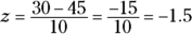 . This means a 30-minute commuting time is well below the mean (so it shouldn’t happen very often). The probability that corresponds to –1.5, according to the Z-table, is 0.0668, which means Bob gets to work in 30 minutes or less only 6.68 percent of the time. So, a commute time of 30 minutes represents the 6.68th percentile.
 - If Bob leaves at 8 a.m. and is still late for work, his commuting time must be more than 60 minutes (a time that brings him to work after 9 a.m.), so you want the percentage of time that his commute is above 60 minutes. Percentiles don’t automatically give you the percentage of data that lies above a given number, but you can still find it. If you know what percentage of the time he gets to work in less than 60 minutes, you can take 100 percent minus that time to get the percentage of time he gets to work in over 60 minutes. First, you standardize 60 to
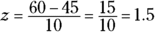 and find the probability that goes with that, 0.9332. Then take
  . If he leaves at 8 a.m., he will be late 6.68 percent of the time.
The answer to Part B is the same as the answer to Part A by symmetry of the normal distribution. The values 30 and 60 are both 1.5 standard deviations away from the mean, so the percentage below 30 and the percentage above 60 will be the same.
18 No. It means your exam score is 0.90 standard deviation above the mean, or in other words,![]() . You have to look up 0.90 on the Z-table to find its corresponding percentile, which is 0.8159; therefore, 81.59 percent of the exam scores are lower than yours.
. You have to look up 0.90 on the Z-table to find its corresponding percentile, which is 0.8159; therefore, 81.59 percent of the exam scores are lower than yours.
Make sure you keep your units straight. A z-score between zero and one looks a lot like a percentile; however, it isn’t!
19 The median is the value in the middle of the data set; it cuts the data set in half. Half the data fall below the median, and half rise above it. So, the median is at the 50th percentile. (See Chapter 5 for more on the median.)
20 If his score is right at the mean, Layton scores in the 50th percentile. So if Layton’s score is above the mean, his standard score is positive, and the percentage of values below his score is greater than the 50th percentile.
21 This problem essentially asks for the score that corresponds to the 60th percentile (the tricky part is recognizing this). First, you look up the standard score for the 60th percentile. The closest value to 0.60 in the Z-table is 0.5987, which matches with a z-value of 0.25. Using the reworked z-formula to solve for x, you get ![]() .
.
22 The wording “10 percent of his fastest times” indicates that only 10 percent of his times are less than his current one; therefore, the percentile is the 10th (not the 90th). The standard score for the 10th percentile is found by seeking out 0.10 in the Z-table. The closest value to this is 0.1003, which matches up with a z-value of –1.28. Converting this back to the original units, you get ![]() minutes. Jimmy has to walk a mile in 6.72 minutes to get into his top 10 percent.
minutes. Jimmy has to walk a mile in 6.72 minutes to get into his top 10 percent.
23 You know the percentile, and you want the original score. The middle step is to take the percentile, find the standard score that goes with it, and then convert to the original score (x) with the z-formula solved for x. In this case, you have a percentile of 42. The standard score for the 42nd percentile is found by seeking out 0.42 in the Z-table. The closest value to this is 0.4207, which matches up with a z-value of –0.20. Converting this back to the original units, you get ![]() . It takes Deshawn about 38.8 minutes to finish the exam.
. It takes Deshawn about 38.8 minutes to finish the exam.
24 Because the top 20 percent of scores get As, the percentage below the cutoff for an A is ![]() . The standard score for the 80th percentile is found by seeking out 0.80 in the Z-table. The closest value to this is 0.7995, which matches up with a z-value of 0.84. Converting 0.84 to original units (x) with the z-formula solved for x, you have
. The standard score for the 80th percentile is found by seeking out 0.80 in the Z-table. The closest value to this is 0.7995, which matches up with a z-value of 0.84. Converting 0.84 to original units (x) with the z-formula solved for x, you have ![]() . The cutoff for an A is 79.2.
. The cutoff for an A is 79.2.
Whatever Z-table you use, make sure you understand how to use it. The Z-table in this book doesn’t list every possible percentile; you need to choose the one that’s closest to the one you need. And just like an airplane where the closest exit may be behind you, the closest percentile may be the one that’s lower than the one you need.
25 The longest 25 percent are the 25 calls with the biggest values. The lengths of calls below the cutoff are 75 minutes, which is the percentile (percentile is the area below the value). The standard score for the 75th percentile is found by seeking out 0.75 in the Z-table. The closest value to this is 0.7486, which matches up with a z-value of 0.67. Converting 0.67 to original units (x) with the z-formula solved for x, you have ![]() . So the cutoff for the longest 10 percent of customer service calls is roughly 12 minutes.
. So the cutoff for the longest 10 percent of customer service calls is roughly 12 minutes.
You may have thought that the z-score here would be –0.67 because it corresponds to the 10th percentile. But remember, the longer the phone call, the larger the number will be, and you’re looking for the longest phone calls, which means the top 10 percent of the values. Be careful in testing situations; these kinds of problems are used very often to make sure you can decide whether you need the upper tail of the distribution or the lower tail of the distribution.
26 I saved the best for last! I consider this problem a bit of an advanced, extra-credit type exercise. It gives you a percent, but it asks you for the standard deviation. When in doubt, work it like all the other problems and see what materializes. You know the percentage of these vehicles getting more than 100 mpg is 20 percent, so the percentage getting less than 100 mpg is 80 (that’s the percentile). The standard score for the 80th percentile is found by seeking out 0.80 in the Z-table. The closest value to this is 0.7995, which matches up with a z-value of 0.84. You know the standard score, the mean, and the value for x in original units. Put all this into the z-formula solved for x to get ![]() . Solving this for σ (the standard deviation) gives you
. Solving this for σ (the standard deviation) gives you ![]() . The standard deviation is roughly 30 miles per gallon.
. The standard deviation is roughly 30 miles per gallon.
27 First, you should check that X, the number of international travelers, is a binomial random variable. You have a fixed number of trials ![]() , which will each result in a success (international destination) or failure (not international). Because they’re chosen randomly, you can assume their travels are independent. Lastly, the probability of success is a constant
, which will each result in a success (international destination) or failure (not international). Because they’re chosen randomly, you can assume their travels are independent. Lastly, the probability of success is a constant ![]() . So this is a binomial random variable you’re working with. Now check to see whether you can use the normal approximation. You find that
. So this is a binomial random variable you’re working with. Now check to see whether you can use the normal approximation. You find that ![]() and
and ![]() are both greater than 10, so you’re good to continue on.
are both greater than 10, so you’re good to continue on.
You’re looking for ![]() , so you need to standardize the x-value of 80 into its proper z-value. Remember to first find the mean
, so you need to standardize the x-value of 80 into its proper z-value. Remember to first find the mean ![]() and the standard deviation
and the standard deviation ![]() . Putting these into the z-formula, you get
. Putting these into the z-formula, you get ![]() . To solve the problem, you need to find
. To solve the problem, you need to find ![]() . From the Z-table, you can look up that
. From the Z-table, you can look up that ![]() . So, the chance that less than 80 of the next 500 people will be flying internationally is approximately 73.57 percent. (This is a really good approximation because the exact value found with some fancy statistical software is 71.68 percent; the approximation is off by only 1.89 percent.)
. So, the chance that less than 80 of the next 500 people will be flying internationally is approximately 73.57 percent. (This is a really good approximation because the exact value found with some fancy statistical software is 71.68 percent; the approximation is off by only 1.89 percent.)
28 No. This is asking about a binomial random variable where X is the number of children who get on the ride out of the next ![]() riders. When you check to see whether you can use the normal approximation to the binomial, you find that
riders. When you check to see whether you can use the normal approximation to the binomial, you find that ![]() , which is greater than 10. But
, which is greater than 10. But ![]() , which is not greater than 10, so you should not use the normal approximation.
, which is not greater than 10, so you should not use the normal approximation.
And why not? Well, when you calculate the exact binomial probability and the normal approximation in that fancy statistical software, the approximation is actually about 4.5 percent lower than the exact answer. That’s not so good.
29 This exercise should help demonstrate to you why going with the approximation isn’t always best, even if it’s faster.
- First, you should check that X, the number of shots made, is a binomial random variable. You have a fixed number of trials
 , which will each result in a success (shot made) or failure (shot missed). The trials are independent, and the probability of success is a constant
  . So you can use the binomial table (Table A-3) to find
  . Look at the portion of the table where
  and focus on the column where
  . You can rewrite the probability as
  . So there is a 58.8 percent chance that you’ll make at least 10 out of your next 20 shots.
 You know that X is a binomial, so check to see whether you can use the normal approximation. You find that
 and
and  are both greater than or equal to 10. This just barely meets the criteria, so you can go ahead with the approximation.
You’re looking for
 , so you need to standardize the x-value of 15 into its proper z-value. Remember to first find the mean
  and the standard deviation
  .
.Putting these into the z-formula, you get
 . To solve the problem, you need to find
  . You don’t need the Z-table for this one, because you know that
  splits the standard normal in half. So by symmetry,
  . According to this, the chance that you’ll make at least 10 of the next 20 shots is approximately 50 percent.
The approximation is 8.8 percentage points lower than the exact calculation
 . This is partly due to the fact that n is so low. As I cautioned earlier, the approximation works best when n is large. If n isn’t large enough, you may not be able to rely too strongly on your approximations. Recall from Chapter 9 that the binomial distribution is discrete, and in this chapter, you see that the normal distribution is continuous. Some statisticians use a method known as “continuity correction” to work out the change. But better than that, as the value of n increases in binomial distributions, at a distance, it begins to look and behave more like a continuous one. You see much more on this useful idea through the Central Limit Theorem in Chapter 12.
If you’re ready to test your skills a bit more, take the following chapter quiz that incorporates all the chapter topics.
Whaddya Know? Chapter 10 Quiz
Quiz time! Complete each problem to test your knowledge on the various topics covered in this chapter. You can then find the solutions and explanations in the next section.
1 The normal random variable is a discrete random variable. True or false?
2 The Z-distribution has mean _______________ and standard deviation _______________.
3 Suppose test scores have a normal distribution with mean 70 and standard deviation 5. According to the Empirical Rule, about what percentage of test scores passed the test with a grade of more than 60?
4 Suppose test scores have a normal distribution with mean 70 and standard deviation 5. According to the Z-table, exactly what percentage of test scores passed the test with a grade of more than 60?
5 Suppose the miles you get on a certain brand of tire have a normal distribution with mean 40,000 and standard deviation 5,000. What’s the chance that a randomly chosen tire gets more than 50,000 miles on it?
6 Suppose the miles you get on a certain brand of tire have a normal distribution with mean 40,000 and standard deviation 5,000. Ten percent of the tires get more mileage than what value?
7 The weights of Nigerian Dwarf baby goats (aka kids) have a normal distribution with mean 3 pounds and standard deviation 0.5 pound. What is the chance that a randomly chosen baby goat weighs more than 4.5 pounds?
8 My baby Nigerian Dwarf goat weighed 1.75 pounds at birth. What percentile was she at, in terms of weight?
9 Suppose 90% of basketball players graduate from College X. What is the chance that out of 100 randomly chosen basketball players from College X, more than 80 of them graduate?
10 Suppose it is reported that 70% of all college graduates worked at a restaurant sometime during their college experience. You sample 100 college graduates at random. What is the chance that at most 65 of them worked at a restaurant sometime during their college experience?
Answers to Chapter 10 Quiz
1 False. The normal random variable has a continuous distribution (bell-shaped).
2 The Z-distribution has a mean of 0 and a standard deviation of 1.
3 If you passed the test, you scored more than 60. You divide this problem into two parts: the probability of getting 60 to 70 (the mean) and the probability of getting higher than 70. Because half of the probability in a Z-distribution is above the mean, the probability for scoring higher than 70 is ![]() . Because 60 is 2 standard deviations below the mean of 70 (every standard deviation is worth 5 points), the probability for scoring between 60 and 70 is half of 95%. This is because the Empirical Rule tells you that about 95% of the values in a normal distribution are within 2 standard deviations on either side of the mean. You only need one side of the mean, so you take
. Because 60 is 2 standard deviations below the mean of 70 (every standard deviation is worth 5 points), the probability for scoring between 60 and 70 is half of 95%. This is because the Empirical Rule tells you that about 95% of the values in a normal distribution are within 2 standard deviations on either side of the mean. You only need one side of the mean, so you take ![]() . Sum these two probabilities to get
. Sum these two probabilities to get ![]() , or 97.5 percent. This is your approximate answer to the question. Most of the students passed!
, or 97.5 percent. This is your approximate answer to the question. Most of the students passed!
4 You start out with ![]() . Then you standardize 60 to a z-value by taking
. Then you standardize 60 to a z-value by taking ![]() . You want
. You want ![]() ). On the Z-table you go to the row for –2.0 and the column for .00 and you find 0.0228. This is
). On the Z-table you go to the row for –2.0 and the column for .00 and you find 0.0228. This is ![]() . To get
. To get ![]() , you take
, you take ![]() , or 97.72 percent. This is your exact answer to the question.
, or 97.72 percent. This is your exact answer to the question.
5 Here you want ![]() where X is the number of miles you get on the tire. Change to a z-value by taking
where X is the number of miles you get on the tire. Change to a z-value by taking ![]() . Now you find
. Now you find ![]() . Look up 2.00 in the Z-table by finding the row for 2.0 and the column for .00 and intersecting them to get 0.9772. This is
. Look up 2.00 in the Z-table by finding the row for 2.0 and the column for .00 and intersecting them to get 0.9772. This is ![]() . To calculate
. To calculate ![]() , take
, take ![]() . It’s highly unlikely that your randomly chosen tire will last over 50,000 miles.
. It’s highly unlikely that your randomly chosen tire will last over 50,000 miles.
6 Because you know 10% of the tires last more than a certain value, that value is standing at the 90th percentile. If 10% lie above it, then 90% lie below it, and percentiles reflect area below a certain value. To find the 90th percentile for X (the tire mileage), you first find the 90th percentile for Z, then change it to X. The 90th percentile of Z is that value of Z that goes with a value of .90 in the body of the table. Find the value closest to .90, which is 0.8997; then follow it across to determine which row it’s in, and go up to determine which column it’s in. Here you see 0.8997 is in row 1.2 and column .08, so the 90th percentile of Z is 1.28. Now change to X by using the z-formula, and solve for X:
So 90 percent of the tires get at least 46,400 miles on them in this case.
7 Here you are looking for ![]() . Change to Z and get the following:
. Change to Z and get the following: ![]() according to the Z-table (row for 3.0 and column for .00).
according to the Z-table (row for 3.0 and column for .00).
So it’s really unlikely that a baby goat will be that large in this scenario.
8 This is a true example; I have a goat that was born this small. Her name is Half-Pint and she’s doing great! To find her percentile, you find ![]() . You change to Z and get
. You change to Z and get ![]() . Looking at the Z-table you find the row for –2.5 and the column for .00 and you get .0082. So Half-Pint was at the .82th percentile (not the 82nd percentile — this is less than the 1st percentile range.) She was small. But now she’s the herd queen, so go figure.
. Looking at the Z-table you find the row for –2.5 and the column for .00 and you get .0082. So Half-Pint was at the .82th percentile (not the 82nd percentile — this is less than the 1st percentile range.) She was small. But now she’s the herd queen, so go figure.
9 Let X = number of graduating basketball players at College X out of 100 randomly chosen ones. X has a binomial distribution because the players either graduate or not (yes/no); you have a fixed number of trials ![]() ;
; ![]() is the same for each randomly chosen player; the results are independent because you chose them randomly. You are looking for
is the same for each randomly chosen player; the results are independent because you chose them randomly. You are looking for ![]() , which is a tall order for a binomial distribution, because you would have to find
, which is a tall order for a binomial distribution, because you would have to find ![]() and sum them all up. However, you may be able to use the normal approximation if your conditions are met — let’s check. You have
and sum them all up. However, you may be able to use the normal approximation if your conditions are met — let’s check. You have ![]() , which is at least 10; you have
, which is at least 10; you have ![]() , which is at least 10 — whew! The conditions are met. You want
, which is at least 10 — whew! The conditions are met. You want ![]() so you change to Z, which means
so you change to Z, which means ![]() . For
. For ![]() you use np, the mean of the binomial distribution, and for
you use np, the mean of the binomial distribution, and for ![]() you use
you use ![]() . Going back to Z, you have
. Going back to Z, you have ![]() . Go to the row for –3.3 on the table and the column for 0.30 and intersect them. You get
. Go to the row for –3.3 on the table and the column for 0.30 and intersect them. You get ![]() . This is an approximate answer. You’re very likely to get at least 80 players to graduate out of 100 with these circumstances.
. This is an approximate answer. You’re very likely to get at least 80 players to graduate out of 100 with these circumstances.
10 Here X = number of college graduates out of 100 who have worked at a restaurant at some point in their college careers. You want P(X at most 65) where ![]() and
and ![]() . “At most” means less-than-or-equal-to, so you are looking for
. “At most” means less-than-or-equal-to, so you are looking for ![]() . In this case, n is large enough to use the normal approximation to help you out — otherwise, you’d have to find
. In this case, n is large enough to use the normal approximation to help you out — otherwise, you’d have to find ![]() , which is quite arduous. To change to Z, you need to find
, which is quite arduous. To change to Z, you need to find ![]() , which are equal to
, which are equal to ![]() and
and ![]() , respectively. You have
, respectively. You have ![]() . This is an approximate answer, contingent on the conditions being met: 1)
. This is an approximate answer, contingent on the conditions being met: 1) ![]() , which is at least 10; and
, which is at least 10; and ![]() , which is at least 10.
, which is at least 10.