Chapter 4
Some Extensions of the OSG Model
The previous chapters define the OSG model and examine its connections with some main ideas in growth theory. So far, we have been concerned only with one-sector growth models. Consumers also have only two variables to choose. We do not take account of influences of other factors that condition productivity of physical inputs such as technology, natural environment, and socio-economic environment. This chapter extends the OSG model to include exogenous technical change, endogenous time, public goods, home production, population, and environment.
This chapter is arranged as follows. Section 4.1 introduces endogenous technological change into the OSG model. First, we discuss the necessity of taking account of technological change and mention various possible patterns of technological change. Then, specifying the Harrod-neutral technological change, we show that the economic system may experience permanent economic growth in terms of per-capita consumption. In Section 4.2, time distribution is no more fixed. We consider interdependence between time distribution (between leisure and work) and economic growth. We show how leisure time changes as the economy grows. Section 4.3 simulates the growth model with leisure proposed in Section 4.3. In Section 4.4, we introduce infrastructures (or public goods in general) into the OSG model. Assuming that infrastructures affect both the production sector and consumers, we show that the dynamic system may exhibit increasing or decreasing returns, depending on how infrastructures enter the production function. Section 4.5 deals with the issues that are seldom mentioned in the traditional growth literature. The OSG model takes account of home production. Section 4.6 illustrates a dynamics between environment and economic growth. Our analysis provides some new insights into complexity of environmental issues. Section 4.7 portrays a dynamic economic evolution with endogenous population. Population growth rate is no more treated as a given parameter but considered as an endogenous variable. A large population may either benefit or harm economic growth, depending on various combinations of conditions in the system. Section 4.8 introduces money into the OSG model. Appendix A.4.1 examines the OSG model with endogenous time when the utility function takes on general forms. Appendix A.4.2 confirms the conclusions of Section 4.6.
4.1 Exogenous Technological Change
The OSG model in Chapter 2 excludes technical progress - a major potential source of economic growth. A production function F is generally given in the form of:
where K denotes the amount of services of the capital stock employed at time t, N stands for the employment of labor force, L represents the rate of use of natural resources such as land, and Z is the level of knowledge. The time parameter t is explicitly introduced into the production function in order to treat the impact of social, cultural, and institutional changes upon the productivity of the production sector.
We now mention a discussion by Hicks about whether or not individual production relations can legitimately be aggregated into a production function. Hicks held that this issue belongs to the field of the 'static method in dynamic theory'.1 The problem is as follows. Suppose that we are concerned with a production unit such as an economy, an industry, or a firm. For simplicity, only the case of a single output is discussed. It is assumed that only capital K and labor N are used as inputs in producing output F. We pose the question of whether there is any relation Y=F(K,N) which can be expected to hold, even very approximately, at any point of time during the study period. It should be noted that the form F is determined in such a way that output Y is maximized from any given set of inputs K and N. In a static context, the assumption of the existence of a production function is quite acceptable, although there may be other questionable factors such as continuities. However, there are problems if one assumes the existence of a production function in a dynamic analysis. According to the definition the form of a production function is affected by various forms of technological change which is due to innovation (or imitation), management methods, institutional changes and other changeable factors. Now we will examine how such factors can be taken into account in a dynamic analysis.
The simplest method of introducing technological change in a production function is to assume that progress takes place according to some presumed order. As the change is exogenously determined, we can generally describe the changes by introducing a parameter (time) t as Y = F(K,N,t). This form is mostly used in growth models. Production processes may improve as new theories are discovered. But it is to be expected that any immediate progress will be limited as it takes time for people to understand the new theories and to apply them in practice. Alternatively, productivity may be increased owing to innovations introduced by a firm. In order for production to increase to the full extent that the innovation makes possible, a process of adjustment will be needed - a process that will take time. The opportunities which new forms of technology produce take time to be fully realized as the ideas that are generated in this manner have to be transferred from firm to firm. Hicks called this the time needed for informational diffusion. Similarly, it takes time for capital stock to be transmuted into a form which is appropriate to the new technology. This is termed capital transmutation.
How can the processes of such adjustment be described in terms of a production Junction used in dynamic analysis? Hicks suggested that since there are stationary equilibria at dates both before and after the adjustment, it is possible to compare the new equilibrium with the old one. However, this method of comparison tells us little about the dynamic process of adjustment. If the innovation only occurs at the initial point of the study period and there is no other form of innovation to affect the production process during the whole period, we can take account of the effects of the adjustment process and imitation by assuming a functional form such as F(K,N,t), though some costs of learning must necessarily be considered. The problem is that we generally have no idea about when a new theory will be discovered or the time when an innovation may be introduced; they appear to be random to the analyst. In some cases, we may assume that the effects of innovation on production can be treated as small perturbations in a macro sense, and thus the effects can be neglected. We may also introduce a time distribution of innovation and thus the output determined from the production function becomes a random variable. In reality, innovation is more subtle and remains one of the main sources of mystery about technological progress. Rather than dealing with discrete innovations, we can also assume that increases in productivity can be treated as continuous functions of learning by doing and education. Thus, in the long-term, the average effects of innovations are implicitly taken into account. We will take approaches in later chapters. In fact, these approaches (implicitly) mean that there are certain deterministic laws which determine how knowledge can be converted into productivity. We can, at least empirically, know such laws.
Technological change is usually characterized as either endogenous or exogenous, and embodied or disembodied. Endogenous changes which take place according to shifts in the input factors, while exogenous changes occur due to 'manna from heaven'. First, we will discuss exogenous forms of technological change. In this case, the production function takes the form of Y=F(K,N,t), where F is continuous with respect to K, N and t. To classify disembodied and exogenous forms of technological change, let us define an index:
I=(FKKFNN)d(FNN/FKK)dt.
Here, the relative share of capital is defined by FKK / Y; the relative share of labor by FNN / Y. Technological change is defined as: (1) neutral iff the relative shares remain constant and I = 0; (2) labor saving (labor using) iff the relative share of labor falls (rises) and I < 0 (I > 0); and (3) capital saving (capital using) iff the relative share of capital falls (rises) and I > 0 (I < 0). These definitions are dependent on the path designated. For instance, neutral forms of technological change can be further classified as Harrod neutral if the capital-output ratio is constant; Hicks neutral if the capital-labor ratio is constant; and Solow neutral if the labor-output ratio is constant. We now discuss the neutral types of technological changes in detail.
A technical progress is called Hicks neutral if the output isoquant shifts inwards in such a way that the ratio of the marginal products remains unchanged when the capital-labor remains unchanged. This type of technical change can be expressed by:
where A(t) is the index of technical progress. If the production function is taken on the Cobb-Douglas form, we have:
F(t)=AemtKαNβ,
where m is the rate of technical progress and A is a constant.
Solow neutral technical progress occurs when the output isoquant shifts in such a way that the labor-output ratio remains unchanged when the marginal product of labor is unchanged. This technical change is capital-augmenting as it allows the same output to be produced with the same labor and less capital. It can be generally expressed as:
F(t)=F(A(t)K(t), N(t)).
In the case of the Cobb-Douglas production function F(t) = (A(t)K)α Nβ.
Different from Solow neutral technical progress, Harrod neutral technical progress occurs when the output isoquant shifts in such a way that the capital-output ratio remains unchanged when the marginal product of capital is unchanged. This technical change is labor-augmenting as it allows the same output to be produced with the same capital and less labor. It can be generally expressed as:
F(t)=F(K(t), A(t)N(t)).
In the case of the Cobb-Douglas production function:
F(t)=Kα(A(t)N)β.(4.1.1)
We now consider the effect that technical progress has in the OSG model. Let us consider the case of a Harrod neutral technical progress with A(t) = Aemt (where A is a constant). Dividing equation equations (4.1.1) by N(t) gives the per capita production function:
f(t)=Aβkαeβmt.
A continual rise in eβmt at rate βm will result in a continual upward shift in the production function and hence produce long-run growth in output per capita for any given capital-labor ratio. If we denote effective labor at time t by N̄(t) = A(t)N(t), the growth rate of the effective labor force is:
gˉN=m+n.
Effective labor grows at rate m + n, rather than n.
To find the corresponding basic growth equation of the OSG model, we introduce ratio of capital and effective labor as follows:
ˆk(t)≡K(t)A(t)N(t).
Output per effective labor is given by f̂(t) = k̂α. Calculate:
˙ˆk(t)=1AN˙K(t)−(n+m)ˆk(t).
With this equation, capital accumulation equation (2.4.4) becomes:
˙ˆk(t)=λˆk(t)α-(ξk+n+m)ˆk(t).(4.1.2)
This differential equation is the same as equation (2.4.6). Hence, we conclude the following theorem, corresponding to Theorem 2.5.1.
Theorem 4.1.1 (Growth with Harrod-Neutral technological change)
If δ and λ satisfy:
0<ξk+n+mλ<ˆf'(0),(4.1.3)
then there exists a unique positive equilibrium k̂*, which is asymptotically stable in the region k̂ > 0.
We can illustrate the dynamics similarly as Figure 2.8. It should be noted that as m rises, the equilibrium value of capital per unity effective labor falls. The reason for this is similar to that for reduction of equilibrium value of capital-labor ratio as a consequence of a rise in population growth rate in the OSG model. Different from the OSG model in which the equilibrium values of capital, consumption level per capita are constant in equilibrium, these variables are permanently growing in the same rate as technological change. That is k(t) = k̂* Aemt and c(t) = ĉ* Aemt. Nevertheless, the sense of reality tells us that permanent growth in living standard can hardly happen. We will come back to growth and technological change in late chapters.
It is not difficult to check that similar results hold for the other types of neutral technological change. In the literature of neoclassical growth theory, we can find different forms of technological changes within the Solow framework. As the production side is the same in the Solow model and the OSG model, it is straightforward to introduce these changes as well as analytical conclusions to the OSG model.2
4.2 Endogenous Time and the OSG Model
In most parts of the world the value of their time is very low. Work is hard, wage rate is low, life is harsh. In a few advanced economies, the value of the time is high. As recorded in Schultz, real wages measured in terms of the cost of food are changeable over history, as illustrated in Table 4.1.3 Schultz explained that 'The high price of human time is a clue to many puzzles. These puzzles include the shift in institutional support from the rights of property to that of human rights, the decline in fertility, the increasing dependence of economic growth on value added by labor relative to that added by materials, the increases in labor's share of national income, the decline in hours worked, and the high rate at which human capital increases.'4
Table 4.1 Evolution of Time Values
| 2 weeks of wages in bushels of wheat | |
|---|---|
| Time of Ricardo (1817) England | 1 |
| Marshall's time (1890) United States | 20 |
| Eighty years later (1970) United States | 300 |
| India field laborer in 1970 | 2 |
Not only the value of time is changeable over time and different over space, but also the time distribution between leisure and working is constantly changing as living conditions and work environment are improved. Time saved today on one thing must be spent on another activity or be lost forever. There is no way to stop time flows. The implications of economic rationality in the allocation of time have been made explicit in a formal and rigorous theory of the subject since Becker published his seminal work in 1965.5 There have been studies on the interdependence between the productivity of a person's labor, his income, the price of leisure time and time allocation. There is an immense body of empirical and theoretical literature on economic growth with capital accumulation and endogenous knowledge and on complex of time distribution between home and non-home economic and leisure activities. Since the Solow model has not designed any rational mechanism about behavior of households, we cannot discuss issues related to interdependence between economic growth and time distribution within the Solow approach. Different from the Solow model, the Ramsey model proposes a rational mechanism for explaining behavior of households. It is possible to introduce endogenous time into the Ramsey model. Although most of growth models treat the supply of labor as inelastic, that is, labor is either totally fixed or, alternatively, grows at some exogenously determined rate, there are some growth models with endogenous labor supply.6 The advantage of our approach over the Ramsey approach is evident in that the resulted dynamic analyses in our approach are far more tractable than the Ramsey approach.
On the basis of labor and family economics, this section treats time allocation between working and leisure time as endogenous variables. Here, leisure time means time at home. Accordingly, leisure time may be used as home service production and pure leisure. We propose a dynamic interdependence of saving, consumption and time allocation on the basis of the one-sector growth model developed in Chapter 2. This section is a simplified version of the dynamic trade model with time distribution proposed by Zhang in 1995.7
The production aspects of the economic system are similar to the one-sector growth model. The parameters, N, δk, ξ, λ, variables, K(t), F(t), S(t), C(t), r(t) and w(t), are defined the same as in Chapter 2. We introduce two variables T(t) and Th(t) to stand for the working time and leisure time of each worker. We assume that labor and capital are always fully employed. The total labor force N*(t) is given by N*(t) = T(t)N. Here, we omit any other possible impact of working time on productivity. For instance, if over-working reduces productivity per unity of working time, it is much more complicated to model the qualified labor force and working time. The production function of the economy is specified as:
F=KαN*β, α + β=1.
The marginal conditions are given by:
r(t)=αF(t)K(t), w(t)=βF(t)N*(t).(4.2.1)
The current income Y consists of the wage income and payment interest for its capital, i.e.:
Y(t)=r(t)K(t)+w(t)T(t)N.
By equation (4.2.1), we have Y(t) = F(t). The gross disposable income is Y*(t) = Y(t) + K(t). As in Chapter 2, the budget constraint is:
C(t)+δkK(t)+S(t)=Y*(t)=r(t)K(t)+w(t)T(t)N+K(t).
The time constraint requires that the amounts of time allocated to each specific use add up to the time available T(t) + Th(t) = T0. Substituting this equation into the above budget constrain yields:
C(t)+w(t)Th(t)N+S(t)=ˆY(t)
where:
ˆY(t)=r(t)K(t)+w(t)T0N+δK(t), δ≡1-δk.
The disposable personal income is the sum of the income from interest payment, r(t)K(t), 'maximum' wage income, w(t)T0N, with the given wage rate (which is the wage income earned when all the time available is devoted to work), the current wealth, K(t), and the depreciation of capital δkK(t). At each point of time, disposable personal income is allocated among current consumption C(t), 'lost income' due to leisure, w(t)Th(t)N, and saving, S(t).
We assume that at each point of time consumers' preferences over leisure time, consumption and saving can be represented by the following utility function:8
U(t)=Tσh(t)Cξ(t)Sλ (t), σ, ξ, λ>0,
where σ is called propensity to use leisure time, ξ, propensity to consume, and λ, propensity to own wealth. For simplicity, we assume these propensities to be fixed.9 For consumers, wage rate w(t) and rate of interest r(t) are given in markets and wealth K(t) and the depreciation δkK(t) are predetermined before decision.
Consumers' problem is to choose current consumption, leisure, and saving in such a way that utility levels are maximized. Maximizing U(t) subject to the budget constraints yields:
w(t)Th(t)N=σpˆY(t), C(t)=ξρˆY(t), S(t)=λρˆY(t),(4.2.2)
ρ≡1σ + ξ + λ.
These conditions say that the total leisure measured in wage is proportional to the disposable personal income with the proportional rate being equal to the propensity to enjoy leisure. Similarly, the optimal consumption and saving are proportional to the disposable personal income.
The change in the households' wealth is equal to the net saving minus the wealth sold at time t, i.e.:
˙K(t)=S(t)-K(t).
By equation (4.2.3), K(t) evolves according to:
˙K(t)=λˆY(t)-K(t).
As output is either consumed or saved, we have:
C(t)+S(t)-K(t)+δkK(t)=F(t),
where C(t) is consumption and S(t) - K(t) + δkK(t) is equal to net saving. We show now that this equation is redundant. Using:
ˆY(t)=Y(t)+δK(t),
we see that the above equation is the same as the budget constrain. This means that the relationships expressed in this equation are contained in Y(t) = F(t), Ŷ(t) = Y(t) + δK(t), and the budget constraint. We thus omit this equation in later discussions.
We have built the dynamic model. The dynamics consist of one-dimensional differential equation for K(t).
In order to analyze the properties of the dynamic system, it is necessary to express the dynamics in terms of one variable at any point of time. From:
˙K(t)=λˆY(t)−K(t),
and the definition of Y(t), it is sufficient to express T(t) or Th(t) as functions of K(t). To show this, first we substitute:
r(t)=αF(t)K(t), w(t)=βF(t)N*(t),
into Th(t) = σŶ(t)/w(t)N in equation (4.2.1). We get:
βNThσρK-βT0NK=αN*K+δN*F,
where the definition of Ŷ(t) is used. From the definition of N* and T + Th = T0, we have N*(t) = (T(t) - T0)N. Substituting this equation into the above equation yields:
Φ(Th)≡(T0-Th)αδNαKα-ˉαThNK+T0NK=0,(4.2.3)
where we use F=KαN*β and ˉα≡β/σp+α>1. It is straightforward to show that for any K(t) > 0, the equation ϕ(Th(t)) = 0 has a unique solution for 0 < Th(t) < T0. That is, we can consider Th(t) as a unique function of K(t). We thus obtain the following lemma.
Lemma 4.2.1
The dynamics are given by the following differential equation:
˙K(t)=λˆY((t))-K(t)=λY(t)-(1-δλ)K(t),
where Y(t) is a function only of K(t). The variables are uniquely determined as functions of K(t) at any point of time by the following procedure: Th(t) by equation (4.2.4) → T(t) = T0 - Th(t) → N*(t) = T(t)N → F(t) = K(t)α N(t)*β → r(t) = αF(t)/ K(t) and w(t) = βF(t)/ N*(t) → Ŷ(t) = Y(t) + δK(t) → C(t) and S(t) by equation (4.2.2).
Equation (4.2.3) implies that as the economy becomes richer, people will choose longer leisure hours if their preference structures remain the same. To see how wealth may affect time allocation, we take derivatives of equation (4.2.3) with respect to K:
dThdK=δβTαT−βδK+ ˉαKαNβ>0.
This result does not seem to be held in economies such as Taiwan and Hong Kong, where people tend to work longer hours as they become richer. This comes from our hypothesis that preference structures are invariant over time. In reality, as people become richer, their desires for holding wealth may become stronger (or weaker). We consider a case that people's propensities to enjoy leisure time and to consume are invariant but their propensities to hold wealth increase as they become richer. That is, ξ and σ are constant and λ(K) is a function of K. It is easy to show that the impact of wealth on time allocation is:
dThdK=δβTα-(βThKαNβ/σˉα)dλ/dKδKT−β+ ˉαKαNβ.
If consumers' preference change is characterized by dλ / dK < 0, then they will allocate more time to leisure as they accumulate more wealth. On the other hand, if economic growth strengthen consumers' desires for holding wealth, i.e., dλ / dK > 0, then the sign of dTh / dK is ambiguous. With proper consideration of taste changes, the model can explain positive as well as negative relationships between leisure time and wealth.
The growth rate of the current income is:
gY≡˙YY=(αK-βTdThdK)˙K,(4.2.4)
where we use:
˙T=-˙Th=-˙KdThdK.
We see that even when wealth rises, the national income may decline because consumers will devote less time to work. But in the case of dTh / dK < 0, an increase in K will always be associated with an increase in the national current income.
We mentioned that value of time, measured by w (= βF / N*α), has increased. The evolution of value of time follows:
gw=˙ww=α(˙KK-˙TT)=(1+δβδ+ˉαF/K)αgK,
where we use equation (4.2.4). Value of labor's time rises (falls) as wealth rises (declines).
The differential equation K̇ = λŶ(K) - K, determines the motion of K(t). As all the other variables in the system are uniquely determined as functions of K(t), it is sufficient to examine the dynamic properties of the above differential equation.
We now examine some properties of the dynamic system. In equilibrium λŶ(K) = K. We have the following proposition.10
Proposition 4.2.1
The dynamic system has a unique stable equilibrium. The variable K is given K=TN/ˉλ1/β, where ˉλ≡ξk/λ. All the other variables are given by the procedure given by Lemma 4.2.1.
Since there are no increasing returns effects in time allocation, the system behaves like the OSG model. The following two corollaries summarize the effects of change in the propensities to enjoy leisure and to hold wealth on the economic structure in equilibrium.
Corollary 4.2.1
If the propensity σ use leisure time rises, working time, consumption level and level of capital stocks are reduced, and the total output is reduced. The wage per unity of time and the rate of interest are not affected by changes in σ.
Corollary 4.2.2
If the propensity λ to own wealth rises, the worker's working time, the total level of capital stocks and the total output increase, the consumption level may either rise or fall, the rate of interest falls, and the wage rate rises.
We defined the OSG model with endogenous time when both production function and utility function are taken on the Cobb-Douglas form. In Appendix A.4.1, we generalize the model in that the functions are in general forms.
4.3 Simulating Evolution of Time Value and Distribution
The previous section shows that as people become richer, they tend to consume more leisure time. Nevertheless, economic history does not confirm this positive relationship between economic growth and leisure time. It is known that as people become richer, they may either consume more or less leisure time, depending on preference and other conditions. In this section, we will simulate the model to illustrate different patterns of time value and distribution over time.
For illustration, we summarize the model in the previous section. The production sector is described by r = αF / K and w = βF / N*, where F = AKαN*β and N*(t) = T(t)N. As we will introduce some exogenous technological change, we add A(t) to the production function.
Consumers' behavior is described by:
w(t)Th(t)N=σˆY(t), C(t)=ξˆY(t), S(t)=λˆY(t),
where:
ˆY=rK+wN+δK,T+Th=T0=1, ρ=1.
The level of capital stock, K(t), evolves according to:
˙K=λF-(1-δλ)K.
We can consider Th(t) as a unique function of K(t) through:
Φ(Th)≡(T0-Th)αδNαKα-ˉαThNK+T0NK=0,(4.3.1)
where we use F = Kα N*β and ˉα≡β/σ+α>1. We now simulate the model with some specified form of technological change and preference change.
First, we specify the following parameters:
A=0.5, N=1, T0=24, α=0.3, δk=0.03, λ=0.25, σ=0.40.
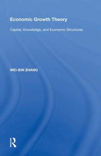
With the initial condition of T(0) = 12, we simulate the motion of T(t), K(t), Y(t), C(t), and w(t) with period of 10 years. Figure 4.1 depicts the motion of these variables during the given period. Figure 4.1a shows that work time declines as time passes. In the initial state, half of the total time is spent on working. Workers gradually reduce work hours. Figure 4.1b shows that capital stock increases over time. The two plots show that capital accumulation moves in the same direction as leisure changes. This can also be confirmed by taking derivatives of equation (4.3.1) to obtain:
˙Th=(T0-Th)α βδNα(T0-Th)−βαδNα + ˉαNKβ˙KK.
As capital stock increases, the current income and the consumption rise. As capital stock increases, time value declines. Figure 4.1c demonstrates that the consumption and the current income rise rapidly in the initial period but the growth rates decline as the system approaches equilibrium. Figure 4.1d predicts that as work time declines, the wage rate declines.
We now examine impact of changes on dynamic processes of the system. First, we examine the case that all the parameters, except ρ, are the same as in Figure 4.1. We reduce the propensity to enjoy time from 0.40 to 0.35. The simulation results are demonstrated in Figure 4.2. The solid lines in Figure 4.2 are the same as in Figure 4.1, representing the values of the corresponding variables when σ = 0.40; the dashing lines in Figure 4.2 represent the new values of the variables when σ = 0.35. Figure 4.2a shows that as the propensity to enjoy leisure falls, work time increases from the initial time rather than declines as in the old situation with σ = 0.40. Figure 4.2b demonstrates that as work time rises, the wealth declines as time passes. Although the wealth declines as time passes in the case of σ = 0.35, the wealth in case σ = 0.35 is more than the wealth σ = 0.40 at each point of time. The reason is that as the propensity to enjoy time falls, the propensity to consume rises (as we fix the propensity to own wealth). As shown in Figure 4.2c, both the consumption and the current income fall as time passes. In Figure 4.2d, we see that the wage rate converges in the long term; but in the initial period, the wage rate in the new case declines as time passes.


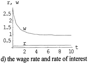
Figure 4.1 Simulating the OSG Model with Endogenous Time
We examine the case that all the parameters, except A, are the same as in Figure 4.1. We consider that the total productivity rises from 0.50 to 0.60. The simulation results are demonstrated in Figure 4.3. The solid lines in Figure 4.3 are the same as in Figure 6.3.1, representing the values of the corresponding variables when A = 0.50; the dashing lines in Figure 4.3 represent the new values of the variables when A = 0.60. We can similarly interpret the new dynamics as we interpreted Figure 4.2. It is shown that as the productivity rises, the work time falls and the value of work time rises.


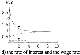
Figure 4.2 As the Propensity to Enjoy Leisure σ Declines From 0.40 to 0.35


Figure 4.3 As the Productivity A Increases from 0.5 to 0.6
It should be noted that another way to explore evolution of time distribution is to consider possibility of value change as an endogenous process of economic evolution. For instance, we may generally propose that the propensity to own capital and the propensity to enjoy time are related to the wealth and current income as:
λ(t)=ϕ(K,Y), σ(t)=ϕ(K,Y),
where φ(K,Y) and φ(K,Y) are proper functions of K(t) and Y(t). The two functions, φ(K,Y) and φ(K,Y), may be taken on different forms because taste changes vary among individuals. Specifying taste change patterns, we can simulate the model.
4.4 Public Goods and Returns to Scale
Infrastructure is public investment in roads, sewers, airports, and even includes education. Infrastructures provides widespread benefits to consumers and raises the return on private investment and productivity of production sectors. It is argued that recent inadequate public investment in infrastructure has been the major cause of the productivity slowdown in the United States. In 1991 Barro found a negative and significant effect of the level of public consumption as a percentage on economic growth rates of countries.11 It is argued that a great government intervention would distort the incentives systems, so that a higher government size would be associated with a lower productivity.
Although he asked for less government intervention, Adam Smith never said that government should not intervene in economic activity at all. The problem is not only how much the government intervenes but also how it spends its resources. Government can affect both physical capital formation and human capital accumulation. Government's expenditures on health, nutrition, and education can be considered as an investment in the sense that they will lead to a more productive force in the future. The quantity and quality of public infrastructure - roads, airports, railways, ports, military defense systems, schools, public hospitals, and the like - are essential for the welfare of people and efficiency of production. It is obvious that infrastructures would affect economic growth, either positively or negatively. Formation of government capital is not necessarily conductive to economic growth as it abstracts private use of capital. It is important for us to show under what conditions an increase in formation of public infrastructures would stimulate economic growth.
This section will introduce (public) infrastructure into the OSG model.12 Production function now includes, together with private inputs, those government inputs that will affect the level of output. For simplicity, we only consider a single type of public physical capital. The economy consists of industrial and public sectors. The industrial sector is the same as in the OSG model, except that infrastructures will affect productivity. The population is constant and homogenous; each worker is employed in either of the two sectors. Production function is
F(t)=Gv(t)Kαii(t)Nβii(t), αi+βi=1, αi, βi>0,v≥0,
where αi, βi, and v are parameters, and
- F(t) = the output of the industrial sector at time t;
- Ki(t) = the capital stocks employed by the industrial sector;
- Ni(t) = the labor force employed by the industrial sector; and
- G(t) = the (service) level of the public sector.
It should be noted that G(t) is often interpreted to be generated by learning-by-doing or human capital spill-over effects. We now interpret the variables as public goods such as physical and institutional infrastructures. The aggregate public goods G(t) is supplied by the government and is taken as given by the firms. Despite increasing social returns to scale, the function allows to maintain the assumption of perfect competition in the goods market since the technology exhibits constant returns to scale for any given level of public goods, which firms cannot control. It is reasonable to consider that production efficiency will be improved as service level of the public sector is improved, it seems that doubling the service level will not double the output with fixed Ki(t) and Ni (t). That is, the parameter V should be less than one. Because public service is freely available to firms, it is not a decision variable for the industrial sector.
The government finances the public sector by imposing taxes on, for instance, the outputs of the firms, the capital income, the labor income, and consumptions. We assume that the government imposes taxes only on the firms.13 The after-tax returns of capital and labor at time t are given by:
r(t)=(1-τ)αiF(t)Ki(t), w(t)=(1-τ)βiF(t)Ni(t),(4.4.1)
where r(t) is the rate of interest, w(t) is the wage rate, and τ (1 > τ ≥ 0) is a fixed tax rate on the producers.
The current income is:
Y(t)=r(t)K(t)+w(t)N.
Since there is no charge for consuming public goods, consumers are faced with the same budget as in the OSG model:
C(t)+S(t)=ˆY(t),
where C(t), S(t), and Y(t) (= Y(t) + δK(t)) are defined as in Chapter 2. Since the level of public services affects welfare of the population, it is necessary to take account of public services in describing behavior of consumers. We specify utility functions as follows:
U(t)=G(t)ϑC(t)ξS(t)λ, ϑ, ξ, λ>0,
where ξ, and λ are defined as before and ϑ is called the propensity to consume public goods. Consumers maximize the utility function subject to the budget constrain. The optimal solution is:
C=ξρˆY, S=λρˆY,
where ρ ≡ l/(ξ + λ) Substituting S = λρŶ into K̇ = S - K yields:
˙K=λρY-δ*K,
where δ* ≡ ξkρ.
We now describe the public sector. In this model, we assume that the public sector is financially supported by the government's tax income. The capital stocks and workers employed by the public sector are paid at the same rates that the private sector pays the services of these factors. This is possible because factor markets are free and competitive. The government may have various objectives in providing public services. It is commonly assumed that the government will maximize the social welfare over certain period of time in determining scales and scopes of its intervention. There are different ways that the government may make 'intervention' in the economic system. In this initial stage - also because we are mainly concerned economic growth, we will not complicate the public sector. There is a production function relating public services with factor inputs. The public sector has a fixed income, because the tax rate is fixed and the public sector has no income resource except the private sector. The public sector is assumed to behave effectively in the sense that it will use the income to maximize public services. We neglect possible inefficiency, such as official corruption, of the public sector.
The public sector supplies public goods by utilizing capital, Kp(t), and labor force, Np(t), as follows:
G(t)=Kαpp(t)Nβpp(t), αp+ βp=1, αp, βp>0.
For the given tax rate τ, the public sector is faced with the budget constraint wNp + rKp = τF. Maximization of public services under the budget constraint yields αpNp / βpKp = r / w. From the above equation and equation (4.4.1), we have:
αpNp(t)βpKp(t)=αiNi(t)βiKi(t).(4.4.2)
The factors are fully employed:
Ni(t)+Np(t)=N, Ki(t)+Kp(t)=K(t).
We have thus built the model. It can be shown that the dynamics is governed by the one-dimensional differential equation:14
˙K(t)=λρnK(t)x + 1-δ*K(t),(4.4.3)
where x ≡ αi + αpv - 1 and:
n≡(ατ0)αNβNνβpp(ττ0αp1-τ)ναp, τ0≡1-τα + βτ-βpτ>0, β0≡β+βpτ1-τ.
Theorem 4.4.1
The dynamics of the economic system are governed by the one-dimensional differential equation (4.4.3). The values of all the other variables are uniquely determined at any point of time for any given positive value of K(t). The dynamic system has a unique equilibrium. Moreover, if x < (>) 0, the unique equilibrium is stable (unstable). In the case of x = 0, capital stock grows at a constant rate, i.e. gK = λρn - δ*. The proof is straightforward. The unique steady state is given by:
K=(δ*λρn)1/x.
Taking derivatives of the right-hand side of equation (4.4.3) and then evaluating the resulted equation at the steady, we get the stability conditions. We illustrate the stability conditions in Figure 4.4.
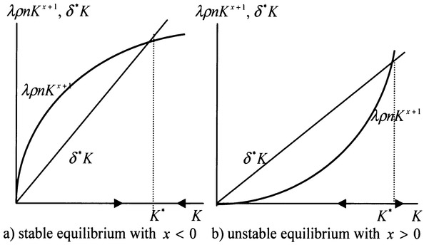
Figure 4.4 Stable and Unstable Steady States
The parameter x determines stability of the system. From x = αi + αpv - 1, we see that this parameter measures net increasing returns to scale in capital accumulation. For instance, let us examine what happen to the capital accumulation equation when we double capital stocks. If we double the capital stocks, then capital inputs in the two sectors are exactly doubled because of the Cobb-Douglas technologies and perfectly competitive input factor markets. The level of public service is 2αp times as many as the old level of services because capital input is doubled. This means that productivity of the industrial sector is αpv times as high as the old level. On the other hand, the output will increase αi times as many as the initial output because of increase in capital stocks in the industrial sector. Consequently, as the total capital doubles, the total output will be 2αi + αpv times as many as before. We see that if αi + αpv < (>) 1 (that is, x < (>) 0), the capital accumulation exhibits increasing (decreasing) returns in scale. If the capital accumulation exhibits decreasing returns to scale, the system becomes stable.
We now examine growth rates of the economy. The model in this section can also generate a persistent growth rate in per-capita consumption. If x = 0, like the AK model, the economy grows permanently at a constant growth rate. In particular, percapita consumption grows according to:
If λρn > δ* then gc is positive. It can be seen that if x = 0, the government can properly choose the tax policy such that gc > 0. It is straightforward to confirm:
dgcdN=(1+x)λρnN>0.
This implies that a highly populated economy, once on track of economic growth, would enjoy a higher economic growth rate than a less populated economy. The impact of population size is due to the effects of returns to scale on the economy.
We now discuss growth rates in general cases. As:
C(t)=ξ(F(t)+δK(t)),
and the population is constant, per-capita consumption growth rate is:
gc(t)=˙c(t)c(t)=αPvF(t)˙Kp(t)/Kp(t) + αiF(t)˙Ki(t)/Ki(t)+δ˙K(t)F(t)+ δK(t),
where we use the fact that labor distribution is invariant with time. Using equations (4.A. 1.1) and (4.4.3), and F(t) = nK1 + x, we get:
gc(t)=(l+g*(t))(λρnKx-δ*),(4.4.4)
where:
g*(t)=xnKxnKx+ δ.
By the definition of g*(t), l + g*(t) > 0 for any X . The direction of change in c(t) is the same as the sign of (λρnKx - δ*). In the case of x < 0, we see that the growth rate is positive when the level of capital stocks is low. The growth rate gradually declines as K(t) rises. Then, gc(t) becomes negative as K(t) further increases - accurately, as λρnK(t)x > δ*. In the long term, the growth rate, like the Solow model or the OSG model, remains zero permanently. In the case of x > 0, when K(t) is small, the growth rate tends to be negative. This may be considered as a kind of 'poverty traps' - the poorer the economy is, the more difficult it is for the economy to enjoy positive growth. Nevertheless, when K(t) is large (i.e., λρnK(t)x > δ*), the economy will enjoy increasing returns from scale. The economy will enjoy unlimited growth if no additional decreasing returns to scale occur. We see that in the case of x > 0, a big push may play a significant role for economies to escape from poverty traps towards unlimited prosperity. A 'big push' strategy for a poor country is effective, in our model, only when x > 0 and the push is strong enough to guarantee:
λρnK(t)x>δ*.
In reality, the condition x > 0 is often not valid for poor countries because of corruption and inefficiency in the public sector and low efficiency in education. Moreover, we can see that if a push is not big enough, it even endangers the economic growth.
So far, our discussion has proceeded with a fixed tax rate. It is important how the growth rate reacts to changes in variables and parameters at any point of time. Since gc(t) is a function of K(t), we can examine changes in K(t) on gc(t) through:
1nKx−1dgc(t)dK(t)=(1 +xnKxnKx + δ)λρx + (λρnKx-δ*)x2δ(nKx + δ)2.
In the case of x < 0 and λρnKx - δ* < 0, the growth rate is slowed down as K(t) rises; in the case of x < 0 and λρnKx - δ* > 0, the growth rate may be either sped up or slowed down as K(t) rises. In the case of x > 0 and λρnKx > δ*, the growth rate is sped up as K(t) rises; in the case of x > 0 and λρnKx < δ*, the growth rate may be either sped up or slowed down as K(t) rises.
Since gc(t) is a function of τ, we can examine changes in τ on gc(t) through:
dgc(t)dτ=[(1+xnKxnKx+ δ)λρ+xδ(λρnKx- δ*)(nKx+ δ)2]Kxdndτ
where:
1ndndτ=v(1-τ)τ-(αi+ vαp)αpτ0(αi+βiτ−βpτ)2−(βi+ vβp)βp(1−τ)2β0.
We see that it is difficult to explicitly judge the impact of government's intervention on growth rates. In the case that v is large, x is positive, τ is small, and K(t) is low, it seems easy to speed up growth rates by expansion policy. These combined conditions seem to be true for the East Asian 'four little dragons' in the 1970s and 1980s. Strong government intervention in these regions benefited economic growth and improved living conditions of many millions of people in these regions. Another extreme case is that public service has no impact on productivity of the private sector, although the level of public services affects people's welfare. This means v = 0 and x < 0. That is, dn / dτ < 0. In this case, if the country is not rich enough to achieve the steady state, i.e., λρnKx < δ*, improved public services will reduce the economy's growth rate.
In the opposite case that the country is so rich - definitely λρnKx > δ*, that its dynamics is far away from the steady state, it is possible that a generous public policy will stimulate economic growth. Indeed, welfare economies like Sweden and Demark once enjoyed high growth rates in association of expansion of public sector.
The impact of changes in the population on the growth rate is:
dgc(t)dN=[(1 + g*)λρKx+λρnKx-δ*(nKx + δ)2xδKx](βi+vβp)nN.
When the system is near the equilibrium point (i.e., λρnKx - δ* being small), dgc / dN > 0 irrespective of whether x is positive or negative. In the case that the economic dynamics is characterized by increasing returns to scale (i.e., x > 0), a rich economy (i.e., λρnKx - δ* being positive) tends to experience high growth rates as its population rises. In the case of x < 0, a poor country tends to experience high growth rates as its population rises.
We mentioned that the public sector is simple in the sense that it is a clean and effective manager of the given public money. In reality, the government may have different purposes. In general, the requirement of a fixed tax rate is too restrict. We may relax this assumption in different ways. We may choose τ such that the utility level or national output is maximized. It is also possible to choose τ such that the growth rate is maximal for given K(t). This can be done by maximizing gc(t) in equation (4.4.4).
We now examine how the steady is affected by different values of the parameters. First, we examine effects of changes in λ. Steady state K is the intersection point of two curves λρnKx+1 and δ*K. A rise in λ reduces δ* and increases λρn, the effects are illustrated in Figures 4.5 and 4.6.
We see that in the case of x < 0, the traditional view on saving is valid - an increase in the propensity to save tends to increase income. Nevertheless, in the case of x > 0, the steady state is lowed down.
The following corollary summarizes the impact of changes in other variables as the propensity to hold wealth. Its proof is left to the reader.
Corollary 4.4.1
In the case of x < (>) 0, an increase in the propensity to hold wealth, λ, has the following impact on the equilibrium values of the variables: (1) K and Y rise (fall); C may be either increased or reduced; (2) Ni and Np are not affected; (3) Ki and Kp rise (fall); (4) F and G increase (decline); and (4) r falls (rises); and w rises (falls).
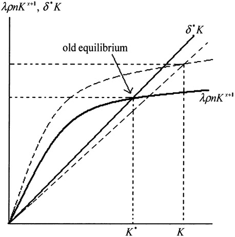
Figure 4.5 The Effects of Increases in λ when x < 0
We may also examine effects of changes in other parameters on the equilibrium values of the variables. How the equilibrium value of capital stock is affected by the tax policy is given by:
xKdKdτ=−v(1-τ)τ+(v-x)βp/β0+(1+ x)αpτ0(1-τ)2.
Since it is difficult to explicitly judge directions of the impact of change in the tax policy, we simulate the model by specifying values of the parameters as follows:
αp=0.4, αi=0.35,v=0.1, δk=0.05, λ=0.65.
As x < 0, the system is stable. As shown in Figure 4.7, when the tax rate is low, the wealth and consumption tend to fall, but the income and output tend to rise as the tax rate is increased. When the tax rate is about 10 percent, a further increase in the tax rate tends to increase the wealth, the current income, and the consumption. Nevertheless, the output of the production sector is reduced.
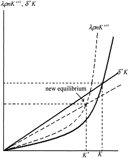
Figure 4.6 The Effects of Increases in λ when x > 0
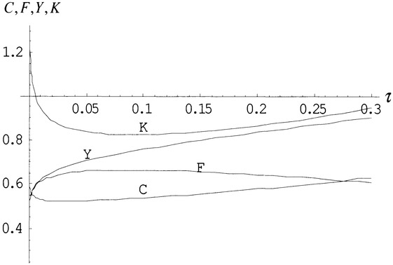
Figure 4.7 The Tax Rate and the Equilibrium Values of C, F, Y and K
4.5 Home Production in the OSG Model
Becker and Lancaster introduced the concept of household production function.15 Instead of receiving utility directly from goods purchased in the market, they assumed that consumers derive utility from the attributes possessed by these goods, and then only after some transformation is performed on these markets goods. A typical example is that the consumers purchase raw food in the market but they derive utility from the consumption of the completed meal, which has been produced by combining the raw food with labor and time in some environment. In Treatise on the Family, Becker emphasized the importance of division of labor and gains from specification.16 Becker applies the concept of household production functions to describe the possibility of producing household commodities with varied inputs. Household commodities include nonmarket goods including children, prestige, envy, health, and pleasures of the senses. These goods are produced with market goods and labor time of household members as inputs. Some goods, such as living space, household heating and lighting and shared automobile trips are jointly consumed and can be considered as local public goods which enter simultaneously into the utility functions of all family members. It is argued that the because of benefits of shared public goods marriage yields a utility surplus over living separately. The well-being of children is treated as a household public good that enters the utility of both parents whether these parents are married or divorces.17 Perceiving household as a firm and applying microeconomic theories about firm behavior to the household, Becker examined specification within the household, comparative advantage, returns to scale, factor substitution, human capital, and assortative mating. Each member of the family can use time either for household labor or market labor and the family can purchase market goods either to consume or to use them as inputs in household production function.
The OSG model in this section views family as production units in economic analysis.18 In addition to enjoyment, households also supply labor services, recreation, spiritual experiences, as well as conventional goods of the do-it-yourself variety. Household activities are conducted within houses as well as outside doors. These activities not only consume goods (like eat fruits and vegetables) but also utilize machines like housing, video, TV, cooking machines, cars, and the like. This section extends the one-sector growth model proposed in Chapter 2 to endogenously determine capital distribution between industrial production and housing.
Except home production, most aspects of this model are the same as the OSG model. The parameters, δk, N, and the variables, K(t), F(t), w(t), r(t) and C(t) are defined as in the OSG model. Total capital, K(t), is distributed between the industrial sector and home use. We denote Ki(t) and Kh(t) respectively the capital stocks employed by the industrial sector and households. The production function is:
Fi(t)=KαiNβ,
where α and β are parameters. The marginal conditions are:
r(t)=αF(t)Ki(t), w(t)=βF(t)N(t).(4.5.1)
We now describe housing production and behavior of households. The current income, Y(t), is:
Y(t)=r(t)K(t)+w(t)N.
We assume that U(t) is dependent on the temporary consumption level C(t), housing conditions Kh(t), and the household's saving S(t), in the following way:19
U(t)=C(t)ξKh(t)ηS(t)λ, ξ η, λ>0.(4.5.3)
Similar to the budget constraint in the OSG model, the budget constraint is
C(t)+r(t)Kh(t)+S(t)=ˆY(t)(=Y(t)+δK(t)).
Maximizing U(t) subject to the budget constraint yields:
C(t)=ξρˆY(t), rKh(t)=ηρˆY(t), S(t)=λρˆY(t),(4.5.2)
where:
ρ≡1ξ + η + λ.
The above equations mean that the housing consumption and consumption of the good are positively proportional to the net income and capital wealth, and the saving is positively proportional to the net income but negatively proportional to the wealth. Substituting S(t) in equation (4.5.2) into K(t) = S(t) - K(t) yields:
˙K(t)=sY(t)-δK(t),
where:
s≡λρ, δ≡ξ0ρ0+δk,ξ0≡ξ+λ, ρ0≡δρ,1>δ>0.
Capital is fully employed:
Ki(t)+Kh(t)=K(t).
As the product is either consumed or invested, we have C + S - K + δK = F.
We have thus built the one-sector growth model with home capital. It can be shown the dynamics can be described by motion of a single variable K(t) as follows:20
˙K(t)=s*F(Λ(K))-δ*K(t),(4.5.3)
where s* = s / ξ0ρ and δ* ≡ δ - ηρ0s*, and A(K(t)) (= Ki(t)) is a function of K(t) determined as a (unique) solution of the following equation:
Φ(Ki)≡αKK−βi-AKαi-ηρ0KρNβ(ξ + λ)=0,
At any point of time, dynamic equation (4.5.3), determines the value of the total capital stocks K(t). We can show that all the other variables are uniquely determined as functions of K(t) at any point of time.
Proposition 4.5.1
For any given (positive) level K(t) of the total capital stocks at any point of time, all the other variables in the system are uniquely determined as functions of K(t). The dynamics of K(t) is given by equation (4.5.3). The dynamic system has a unique stable equilibrium.
The system with home capital has similar dynamic properties with the OSG model, even though its 'internal structure' is more complicated than that of the OSG model. This model provides detailed information about dynamics of the components of national product. The dynamics is illustrated in Figure 4.8. We can explain the behavior as we did with Figure 2.8. It is straightforward to examine impact of changes in any parameter on the equilibrium values of all the variables.
4.6 Environment and Growth21
Energy, natural resources, and environmental pollution are necessary factors of production and consumption. Traditional growth theory neglected issues related to energy, natural resources, and environmental pollution. However, as economics was faced with the challenge of OPEC and the doomsday predictions of the Club of Rome in the 1970s, economists had made efforts to introduce energy, natural resources, and environmental pollution into the neoclassical growth theory. Interactions among capital accumulation and energy, natural resources, and environmental pollution have been examined. In the 1990s, as the new growth theories have been developed, economists have emphasized various implications of knowledge creation and diffusion on dynamics of energy, natural resources, and environmental pollution.
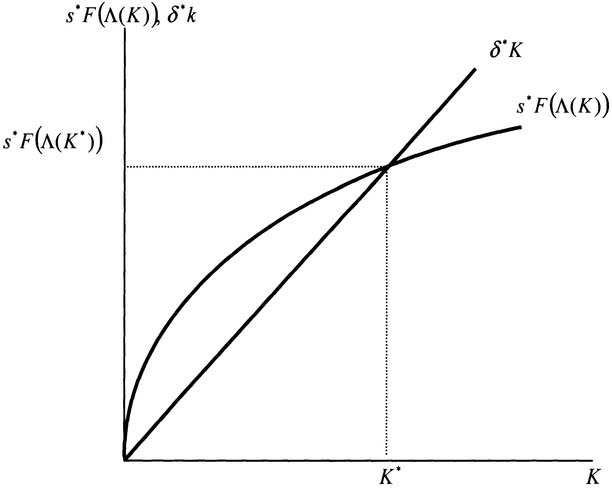
Figure 4.8 Evolution of Capital Stocks in the Home-Production Model
As dynamic interactions among these variables are too complicated, this section provides some insights on economic sustainability by examining tradeoffs between economic growth, consumption, and pollution. We neglect technological change in this initial stage.22 Both production and consumption may pollute environment. Economic growth often implies worsened environmental conditions. Growth also implies a higher material standard of living which will, through the demand for a better environment induces changes in the structure of the economy to improve environment. As a society accumulates more capital and makes progresses in technology, more resources may be used to protect, if not improve, environment. It is well observed that a country in the beginning of its economic development will be experiencing a worsening of the environment, while a country in which growth has taken place over a longer period of time will be adjusting its patterns of growth in such a way that the environment in fact improves. Tradeoffs between consumption and pollution have been extensively analyzed since the publication of the seminal papers by Ploude in 1972 and Forster in 1973.23 Issues related to interdependence between economic growth and environment have been examined from different perspectives.24 This section introduces dynamics of environment and environment policy into the OSG model.
The economic system consists of production and environmental sectors. The production sector is similar to the OSG model in Chapter 2. Only one commodity is produced in the system. The labor distribution is determined by market mechanism. The environmental sector employs labor and capital to purify environment. The government pays the environmental sector's costs of labor force and capital. The government's income comes from taxing the industrial sector. Factor markets are perfectly competitive and labor and capital are always fully employed. The population, N, is fixed. The variables, K(t), F(t), K(t), C(t), S(t), r(t), and w(t), are defined in the preceding section. We introduce:
- Ne(t) and Ke(t) — the labor force and capital stocks employed by the environmental sector;
- E(t) — the level of pollutant stocks; and
- t — the fixed tax rate, 0 < τ < 1.
There are two factor inputs, capital and labor, in economic production. We assume that the environmental quality may affect productivity of production units such as hotels, restaurants and hospitals and deteriorate machines. We specify production function as follows:
F(t)=Ki(t)αNi(t)β exp(-hpE), α + β=1,α, β>0,hp≥0.
The term, exp(-hpE), in F(t) means that productivity is negatively related to the pollution level. We select the commodity to serve as numeraire. The marginal conditions are given by:
r(t)=(1-τ)αF(t)Ki(t), w(t)=(1-τ)βF(t)Ni(t).(4.6.1)
The current income Y(t) is given by:
Y(t)=r(t)K(t)+w(t)N(t).
We now describe dynamics of the stock of pollutants, E(t). We assume that pollutants are created through two sources, production, and consumption. Pollutants may be reduced by two ways. The nature may 'treat' certain pollutants in a similar way to that of waste treatment plants. Some of pollutants may naturally disappear without any human efforts. Pollutants may be treated by using capital and labor. We specify the dynamics of the stock of pollutants as follows:
˙E(t)=qfF(t)+qcC(t)-Qe(t)-q0E(t),
in which qf, qc and q0 are positive parameters and:
Qe(t)=f(E)KueNve,
where u and v are positive parameters, and f(E) (≥ 0) is a function of E. The term qfF means that pollutants that are produced during production processes are linearly positively proportional to the output level.25 The term qcC means that in consuming one unit of the good the quantity qcC is left as waste. The parameter qc depends on the technology and environmental sense of consumers. The parameter q0 is called the rate of natural purification. The term quE measures the rate that the nature purifies environment. The term KueNve in Qe means that the purification rate of environment is positively related to knowledge utilization efficiency, capital and labor inputs. The function f(E) in Qe(t) = f(E)KueNve implies that the purification efficiency is dependent on the scale of pollutants at time t. It is not easy to generally specify how the purification efficiency is related to the scale of pollutants. For simplicity, we specify f as follows f(E) = qeEu where qe > 0 and v > 0 are parameters. The function has the following properties:
f(0)=0,limE→∞ f(E)=∞,dfdE>0, d2fd2E<0.
When E is large, the specified functional form is problematic. At this initial stage of the investigation, we accept the above specified form. In order to describe behavior of households, we define a variable E* = E0 - E, where E0 is called the threshold of pollution level. For instance, consumption of nuclear-generated electricity brings about the creation of radionuclides that cause death or severe mutation when threshold concentrations are exceeded. Electricity production using coal creates atmospheric C02 concentrations which, at sufficiently high levels, may cause dramatic changes. We assume that the critical level is known.26
We assume that the disutility that the society experiences from pollution is a continuous function of the environmental pollution stock. It is assumed that utility level U(t) that a typical household obtains is dependent on the consumption level C(t) of commodity, the environmental condition E*(t) and the saving, S(t). The utility function is specified as follows:
U(t)=E*(t)ςC(t)ξS(t)λ, ς,ξ,λ>0,
in which ζ, ξ, and λ are respectively the propensities to enjoy environment, to consume goods, and to own wealth. As in the OSG model, the budget constraint is:
C(t)+S(t)=ˆY.
The households determine C(t) and S(t) with the level of E*(t) as given. Maximizing U(t) subject to the budget yields:
C(t)=ξρˆY(t), S(t)=λρˆY(t),(4.6.2)
where:
ρ≡1ξ + λ.
It is assumed that the saving is equal to investment. Substituting S(t) in equation (4.6.2) into K̇(t) = S(t) - K(t) yields:
˙K(t)=λρY(t)-ξkρK(t)(4.6.3)
where ξk ≡ ξ, δkλ. We now determine how the government determines the number of labor force and the level of capital employed for purifying pollution. The government budget is given by:
rKe+wNe=τF.
We assume that the government will employ the labor force and capital stocks for purifying environment in such a way that the purification rate achieves its maximum under the given budget constraint. The government's optimal problem is given by:
Max Qe(t)=f(E)KueNve s.t.: rKe+wNe=τF.
The optimal solution is given by:
rKe=τuv0, FwNe=τvv0F,
where v0 ≡ 1/(u + v). The product of the industrial sector is either consumed or invested, i.e.:
C+S-K+δk K=F.
We assume that labor and capital are fully employed:
Ki(t)+Ke(t)=K(t), Ni(t)+Ne(t)=N.
We have thus defined the model. We now examine the behavior of the system. First, we show that the dynamics can be represented by a two-dimensional differential equations system.
Lemma 4.6.1
For any given positive levels of K(t) and E(t) at any given point of time, all the variables in the system can be expressed as functions of K(t) and E(t) by the following procedure: Ki and Ke by equation (4.A.4.1) → Ni and Ne by equation (4.A.4.2) → F = KαiNβi exp(-hpE) → r and w by equation (4.6.1) Y = rK + wN → Qe = f(E)KueNve → C and S by equation (4.6.3) → E* = E0 - E.
The lemma is proved in Appendix A.4.2. Lemma 4.6.1 implies that we can represent the dynamics of the economic system in terms of the following two differential equations:
˙K=α0λρKαNβ exp(-hpE)-ξkρK,˙E=λiKαNβexp(-hρE)+qcδξρK-λeEvKuNv-q0E,
where:
α0≡αaββ, λi≡α0(qf+qcξρ), λe≡qeαueβve.
In steady state, we have:
α0λρKαNβ exp(-hpE)=ξkρK,λiKαNβ exp(-hpE)+qcδξρK=λeEvKuNv+q0E.
Proposition 4.6.1
The dynamic system has a unique stable equilibrium in the case of hp = 0.
In the case of hp = 0, it is straightforward to prove the proposition. In the case of hp > 0, it is possible that the system has multiple equilibriums. Here, we limit our discussion to the case of hp = 0.
We now examine effects of the environmental policy on the system. By α0KαNβ=ˉλK, we have:
1KdKdτ=−(1-b)α*(1-q)β,
in which:
α*≡αuα*1+ βvα*2τv0, α*1≡1(1-τvv0-β(1-τ))(1-τ),α*2≡1(1-τvv0-α(1-τ))(1-τ).
As the tax rate is reduced, the level of capital stocks is increased. By equations (4.A.4.1) and (4.A.4.2), the impact on capital and labor distribution are given by:
1KidKidτ=1KdKdτ-α*1uv0>0,1KedKedτ=1KdKdτ+αα*1(1-τ)τ,
1NidNidτ=−vv0α*2<0,dNedτ=−dNidτ>0.
As τ rises, the capital stock Ki of the production sector falls, the capital stock Ke of the environmental sector may be either increased or decreased.
By F=Y=ˉλK and ξK / λ, we have:
1FdFdτ=1YdYdτ=1CdCdτ=1KdKdτ.
The output level F, the current income Y, and the consumption level C are increased as the tax rate falls. By equations (4.6.1), we get:
1rdrdτ=−11-τ+α*-(αv-βu)βv0α*1α*2(1-τ)2,1wdwdτ=−11-τ-αα*β+(αv-βu)αv0α*1α*2(1-τ)2.
4.7 Population and Capital Accumulation
We now suggest a possible dynamics for population growth.27 Except population dynamics, the model is the same as in the OSG model defined in Chapter 2. We will not repeat the assumptions and definitions of the variables. In the Malthusian growth model the population grows at a constant rate times the current population, with no limitations on its resources. The following logistic growth model:
˙N(t)=nN(t)(m-qN(t)),
takes account of the limiting effects of natural resources upon population growth. However, in a human society resources are 'endogenous variables'. To analyze how production affects population growth, Haavelmo in 1954 suggests the following model:28
where Y(t) is the level of production of the society. Haavelmo further assumed that:
Y(t)=N(t)θ,
where 0 < θ <1.
This population model is valid for an agricultural economy where no capital accumulation is allowed. Zhang extended the Haavelmo population dynamics:29
˙N(t)=nN(t)[C(t)b-qN(t){N(t)Y(t)}θ],(4.7.1)
where n, q, b and θ are non-negative parameters. By equation (2.2.10), we know C = ξY. When b = 0 and q = 0, the model is identical to the Malthusian population model. When θ=0, and q > 0 and b = 0, it is identical to the logistic model. When b = 0 and q > 0, the model is identical to the Haavelmo model. We now interpret our population dynamics. In equation (4.7.1), we interpret Cb as the capacity for supporting the population. This implies that the population which can suitably live (or survive) in a society is dependent upon the current level of consumption. This is similar to the effects of consumption upon the growth rate of the population. The term qN(K / N)θ expresses how wealth makes a contribution as a checking force of the population growth. It means that the richer the society becomes, the more expensive it is for the society to support its people. This is observed clearly in industrialized societies. Surely, this is a description of some possible cases. In some cultures, it is possible to observe the opposite effects of wealth upon population growth. If 0 < b < 1, there are decreasing effects of consumption upon the population capacity. Doubling the current level of consumption will not double the capacity for supporting the people. This case seems acceptable for a developed economy. In a developed economy, each people will consume more because of increased needs for health caring, education, leisure, housing, privacy, and travels. If b > 1, there are increasing effects of consumption upon the population capacity. Doubling the current level of consumption will more than double the capacity for supporting the people. For instance, if people's material consumption consists only simple sheltering and food, it is possible to have situations that double consumption would more than double the capacity. We will see that this parameter plays a key role in determining stability of the dynamics.
The capital accumulation is the same as that in the OSG model. The capital accumulation is characterized by decreasing returns as the population is fixed and a < 1. Although endogenous population is introduced, since a + β = 1 (which does not generate a case of increasing return in the capital accumulation), the system will not exhibit instability if the population dynamics does not exhibit 'increasing returns'. We now look at the population dynamics. Because N(N / F)θ does not exhibit increasing returns in either K or/and N, this term will not create increasing returns in the system. Accordingly, there is only one possible term, Ch for the system to exhibit increasing returns. This happens only when b > 1. We will prove our observation soon. If we consider that b < 1 fits for industrial economies and b > 1 may be suitable for poor countries, we may expect that the system will behave stably like in the OSG model in the case of b < 1; and the system will be unstable, like poverty traps observed in the extended Solow model, in the case of b > 1. From these discussions, we see that b should be considered as an endogenous variable in analysis of economic structural transformation.
According to equation (2.4.4), we know:
˙K=λF-ξkK,
where:
ξk≡ξ+λδk.
By Y(t) = F(t) and F(t) = AKαNβ, the dynamics of K(t) and N(t) are given by the following two-dimensional differential equations:
˙K(t)=λAK(t)αN(t)β-ξkK(t),˙N(t)=nN(t)[ξb(AK(t)αN(t)β+δK(t))b−qN(t)1+αθAθK(t)αθ].(4.7.2)
We specify the parameter values as follows:
α=0.3, δk=0.05, λ=0.65, b=0.3, q=0.4, θ=0.4,A=0.7, n=1.5.(4.7.3)
We simulate the motion of the system with the initial condition K(0) = 1.2 and N(0) = 0.8 for 15 years. In the first few years, the wealth tends to decline but the population grows. After the population reaches 1.45, the growth of the population slows down and the wealth begins to increase.
In equilibrium, we know:
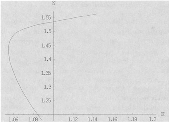
Figure 4.9 The Interaction between the Wealth and the Population
S=KCb=qN1+αθAθKαθ.
Using S/C = λ / ξ solve the above equations:
K=(λAξk)1/βN, N=[A(1+θ)/βq(ξλ)b(λξk)(1+αθ)/β]1/(1−b).(4.7.4)
The Jacobian matrix of the nonlinear system evaluated at the equilibrium is:
J=[−βλFKλβFNJKJN]
in which:
JK≡[(αF+δK)bF+ δK+αθ]nqN2+αθKαθ+1,JN≡[bβFF+ δK-(1+αθ)]qnN1+αθKαθ.
In the case of 0 ≤ b < 1, JK > 0 and JN < 0. The two eigenvalues ϕi, j = 1, 2, are given by:
where:
b1≡βλF2K-JN, b2≡(1-b)nqβλFN1+αθKαθ+1.
In the case of 0 ≤ b < 1, b1 > 0 and b2 > 0. That is:
ϕ1,2=−b1±√b21-b2.
Summarizing the above discussions, we conclude the following proposition.
Proposition 4.7.3
The dynamic system has a unique equilibrium. If 0 ≤ b < 1, then the unique equilibrium is stable. If b > 1, then the equilibrium is unstable.
Finally, we simulate how the equilibrium changes with parameters. First, we examine how the propensity to own wealth determines the long-term equilibrium.
We specify the parameter values, except for λ, as in (4.7.3). In Figure 4.10, we show how the variables change as λ rises from 0.2 to 0.85. Figure 4.10a depicts the variation of 'aggregated variables', K, N, F and C. As the propensity to own wealth rises, the wealth, the population, the consumption, and the output rise. Figure 4.10b shows that the wealth and output per worker are increased. As λ rises, the consumption per capita increases when the propensity to own wealth is low but declines when λ becomes large.

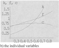
Figure 4.10 The Equilibrium Values for 0.2 ≤ λ ≤ 0.85
Fixing λ = 0.65 and accepting the parameter values, except for A, specified in (4.7.3), we illustrate the impact of change in A with Figure 4.11. As the productivity is improved, the wealth, the population, the total consumption, the output, and the wealth, the output, and consumption per capita are increased. As the population grows more slowly than the wealth, the total consumption and the output, the wealth, the consumption and the output in terms of per capita are increased.

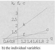
Figure 4.11 The Equilibrium Values for 0.5 ≤ A ≤ 2
Still fixing λ = 0.65 and accepting the parameter values, except for q, specified in (4.7.3), we illustrate the impact of change in q with Figure 4.12. We see that the values of all the aggregated variables decline as the checking force becomes stronger. Figure 4.12 shows that the values of the wealth, the consumption, and the output per capita remains invariant as the checking force changes.

Figure 4.12 The Equilibrium Values for 0.2 ≤ q ≤ 0.8
We now examine how the equilibrium values of the population and consumption per capita are affected by changes both in the productivity and the propensity to save. Accepting the parameter values, except for q, specified in (4.7.3), we illustrate the impact of changes in λ and A with Figure 4.13.

![Figure 4.13 The Simulation Results for λ ∈ [0.2,0.85] and A ∈ [0.5, 2]](http://images-20200215.ebookreading.net/10/5/5/9781351159425/9781351159425__economic-growth-theory__9781351159425__Images__fig00076.jpg)
Figure 4.13 The Simulation Results for λ ∈ [0.2,0.85] and A ∈ [0.5, 2]
4.8 Money and Economic Growth
Modern analysis of the long-term interaction of inflation and capital formation begins with Tobin's seminal contribution in 1965. Tobin deals with an isolated economy in which 'outside money' competes with real capital in the portfolios of agents within the framework of the Solow model.30 Since then, many models of growth model of monetary economies are built within the OLG framework.31 This section introduces money within the OSG framework proposed in this study. We present the model in discrete time, numbered from zero and indexed by t = 0, 1, 2, ... Time 0, being referred to the beginning of period 0, represents the initial situation from which economy starts to grow. The end of period t - 1 coincides with the beginning of period t; it can also be called time t. We assume that transactions are made in each period. The model assumes that each individual lives forever. The population, N, is constant. Each individual supplies one unit of labor at each time t. Production in period t uses amount K(t) of capital and amount N of labor services as inputs. It supplies amount Y(t) of goods. Here, production is assumed to be continuous during the period, but then use the same capital that existed at the beginning of the period.
Production is made through a neoclassical constant return to scale technology. The real interest rate and the wage of labor are given as before by:
r(t)+δk=f′(k(t)), w(t)=f(k(t))-k(t)f′(k(t)).(4.8.1)
For simplicity of expression, we normalize N = 1. There is some initial capital stock k0 that is owned equally by all individuals at the initial period.
We assume that agents have perfect foresight with respect to all future events and capital markets operate frictionless. The government levies no taxes. Money is introduced by assuming that a central bank distributes at no cost to the population a per capita amount of fiat money M(t) > 0. The scheme according to which the money stock evolves over time is deterministic and known to all agents. With μ being the constant net growth rate of the money stock, M(t) evolves over time according to:
M(t)=(1+μ)M(t-1), μ>0.
At the beginning of period t the government brings M(t) - M(t - l) additional units of money per capita into circulation in order to finance all government expenditures via seigniorage. For the seigniorage mechanism to work, injections of the additional units of money take place before the other markets open. Let m(t) stand for the real value of money per capita measured in units of the output good. Then, we may rewrite the above equation as:
g(t)=M(t)-M(t-1)P(t)=μ1+μm(t).(4.8.2)
In this model, money acts as a pure store of value. The demand for money relies exclusively on the speculative conjecture that the future exchange value of money in terms of goods will be positive because people will express a positive demand for money in the future. In the absence of uncertainty and with money not being explicitly required for transaction purposes, this 'bubbly view' implies that in a monetary equilibrium the return on money needs to be equal to the return on competing assets such as claims on productive investment projects. In period t, each consumer receiving the per capita nominal money stock M believes that money will be exchanged at the expected future price pm (t + l) > 0. The price of money pm(t) is in terms of goods or it expresses the amount of goods that can be purchased by one unity of money in each period t. According to the definitions, we have: P(t) = 1/ pm(t) A necessary condition for a monetary economy to exist is that the price of money must be positive. If money has a positive value, people have an opportunity to save in money. According to the definition of the price of money, the deflation rate P(t)/P(t + l) coincides with the real return on money. In a competitive economy the absence of arbitrage opportunities entails equality of return on assets:
P(t)P(t + 1)=1+f′(k(t + 1))-δk.
As:
P(t)P(t + 1)=P(t)P(t + 1)M(t+1)(1+μ)M(t)=m(t+1)(1+μ)m(t),
the above balance condition becomes:
1+f′(k(t+1))-δk=m(t+ 1)(1+μ)m(t).(4.8.3)
The consumer obtains income in period t from the interest payment r(t)k(t)and the wage payment w(t):
y(t)=r(t)k(t)+w(t),(4.8.4)
where y(t) is called the current income. We define the disposable income as the sum of k(t) + m(t) and the current income, i.e.:
ˆy(t)≡y(t)+k(t)+m(t).(4.8.5)
The budget constraint is given by:
c(t)+s(t)=ˆy(t).
For simplicity, we take the Cobb-Douglas utility function to describe consumers' preferences:
U(t)=cξ(t)sλ(t), ξ+λ=1, ξ,λ>0,(4.8.6)
in which ξ and λ are respectively the propensities to consume goods and to own wealth. Households maximize utility subject to the budget constraint. We solve the optimal choice of the consumers as:
c(t)=ξˆy(t), s(t)=λˆy(t).(4.8.7)
According to the definitions, the per capita capital in period t + 1, k(t + l) is equal to the saving made in period t minus the real value of money in period t, i.e.:
k(t + 1)=s(t)-m(t).(4.8.8)
The economy starts to operate in t = 0. Each member in period 0 is endowed with M(-l) units of money and owns k0 (= K(0)/ N(0)) units of physical capital. The labor force N is exogenously given. We will show that the above equations allow us to calculate recursively all k(t) and m(t).
We now show that the motion of the system may be expressed in three-dimensional difference equations. Government spending is given by equation (4.8.2). From equations (4.8.5) and (4.8.6), we obtain:
s(t)=λ(y(t)+k(t)+m(t)).(4.8.9)
Substituting equations (4.8.1) and (4.8.4) into the above equation yields:
s(t)=λ(f(k(t))+δk(t)+m(t)),(4.8.10)
where δ ≡ 1 - δk Substituting equation (4.8.10) into equation (4.8.9), we obtain:
k(t+1)=λ(f(k(t))+δk(t)+m(t))-m(t).(4.8.11)
From equation (4.8.3), we obtain:
Definition 4.8.1
Given the initial capital stock k0 and the initial money stock M(-l) a competitive equilibrium is given by a sequence of quantities:
and a sequence of prices (r(t) w(t) P(t)} such that for all periods t - 0,1, 2, ...: (i) competition ensures that factors get paid their marginal products according to (4.8.1); (ii) given M(t) - (l + μ}M(t - l), the budget constraint (4.8.2) of the government is satisfied; (iii) given the price consequence, agents solve optimally the decision problem (4.8.6) subject to c(t)+ s(t) = ŷ(t}. (iv) the evolution of money balances satisfy (4.8.12); (v) investments and saving are matched by (4.8.8); and (vi) all markets clear with the equilibrium conditions being as following:
Labor market: w(t) = f(k(t)) - k(t)f′(k(t));
money market: m(t) = M(t)/ P(t): and
Equilibrium can be further classified as inside and outside money equilibrium: an inside money equilibrium is associated with a situation in which outside balances are zero; an outside money equilibrium is associated with positive outside money balances.
We now examine dynamic properties of the difference equations, (4.8.11) and (4.8.12). At inside money equilibrium with m(t) = 0, we have:
(4.8.13)
Government spending is reduced to zero. As shown before, this system has a unique stable equilibrium given by:
We are mainly interested in monetary economy which is characterized by the three difference equations (4.8.2), (4.8.11) and (4.8.12). As (4.8.11) and (4.8.12) do not contain g(t) we treat g(t) as endogenous variable. In fact, once m(t) is determined, we determine g(t) by (4.8.2).32 Dynamics of the monetary economy are described by (4.8.11) and (4.8.12). We may rewrite the system as follows:
A steady state of the monetary economy needs to satisfy:
From 1 = (l + μ)(δ + f′(k)), we get:
From the properties of f, we see that if δk > μ/(1 + μ), the equation (4.8.17) has a unique solution, denoted by k*. From the first equation in (4.8.16), we solve:
For m* > 0, we should require f(k*)/ k* > ξ / λ + δk. Comparing (4.8.14) and (4.8.18), we see that the monetary economy has a unique equilibrium if:
As:
because of strict concavity of f, f / k strictly decreases in k. Hence, (4.8.19) implies k̄ > k* if both k̄ and k* exist. As f′ decreases in k, we see that if:
then k̄ > k*. In summary, we have the following proposition.
Proposition 4.8.1
Suppose that the inside competitive equilibrium has a unique non-tnvial steady state k̄ > 0. Then, the monetary economy has a unique steady state k* if the following inequality holds: f′ (k̄) < δk - μ/(1 + μ). The steady state is a saddle point.
Proof: We only need to examine the stability of the stead state. The Jacobian at steady state for (4.8.15) is given by:
in which:
The characteristic equation is given by:
where:
We have:
We thus conclude that the two eigenvalues are real and satisfy 0 < ρ1 < 1 < ρ2 The unique monetary equilibrium point is a saddle point.
From (4.8.17), we get:
If the rate of monetary expansion μ is permanently raised, then the per capita capital stock in the new monetary steady state is higher than before. That is, the Tobin effect prevails.33 This is illustrated as in Figure 4.14. As illustrated in Figure 4.14, as μ is shifted, the accumulation equation:
is not affected; the arbitrage relation:
is shifted by lowering the return on real balances via increased inflation taxation. To rebalance the arbitrage relation, the composition of the portfolios of agents needs to readjust in favor of capital. In the new steady state, the capital stock will be higher than before.
Appendix
A.4.1 The General OSG Model with Endogenous Labor
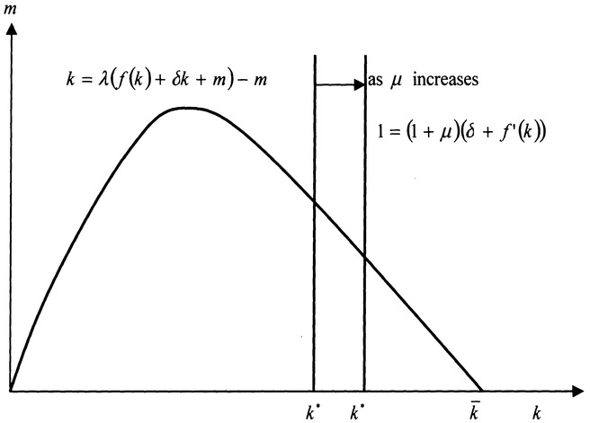
Figure 4.14 The Tobin Effect
We now extend the OSG model with general production and utility functions. As almost all aspects of the model are the same as the model proposed in Section 4.2, we are mainly concerned with technical aspects of the general model. The total labor force N*(t) is given by N*(t) = T(t)N. For simplicity, we specify N = 1. The production function of the economy is:
Assumption A.4.1.1
The production function F: R2+ → R+ is C2 in R2++ and satisfies the following properties:
- i) F(K,N*) is increasing with respect to each argument, homogenous of degree one and concave;
- ii) Fkk(K,N*) < 0 for all N* > 0; and
- iii) and; .
The marginal conditions are given by:
where:
The current income Y consists of the wage income and payment interest for its capital, i.e.:
We have Y(t) = F(t). The budget constraint is:
where:
The utility function is U(t) = U(Th (t),C(t),S(t))
Assumption A.4.1.2
The utility function U(Th(t),C(t),S(t)) is strictly increasing with respect to each argument (Uj(Th,C,S) > 0, j = 1,2,3). It is C2. For all leisure, consumption, and saving levels:
Consumers' problem is to choose current consumption, leisure, and saving in such a way that utility levels are maximized. Construct the Lagrangian:
The first-order condition for maximization is:
The bordered Hessian for the problem is:
The second-order condition tells that given a stationary value of the first-order condition, a positive:
and a negative |H̄| are sufficient to establish it as a relative maximum of U. Under general conditions |H̄2| > 0 is satisfied. The Laplace expansion reduces the bordered Hessian:
(4.A.1.3)
where:
It is straightforward to show that if:
for j ≠ k, j, k = 1, 2, 3, then M12 > 0, M11 < 0, and M14 > 0. That is, |H̄| < 0. If Assumption A.4.1.2 and conditions (4.A.1.4) are satisfied, the maximization problem has a unique solution. We denote an optimal solution as tactions of the disposable income and wage rate:
It is known that the bordered Hessian is identical with the endogenous-variable Jacobian. Hence, if |H̄| is not equal to zero, we can directly apply the implicit function theorem to the problem. That is, the first-order condition has a solution as C1 functions of the disposable income Ŷ and wage rate w.
Taking the derivatives of equations (4.A.1.1) with respect to Ŷ yields:
We solve the impact of changes in Ŷ on the variables as:
By M12 > 0, M13 < 0, M14 > 0, and:
we conclude:
We now examine impact of changes in w on the optimal behavior of households. Taking the derivatives of equations (4.A.1.1) with respect to w yields:
We solve the impact of changes in w on the variables as:
The impact of changes in the real wage rate is ambiguous.
We now find dynamics of capital accumulation. The change in the households' wealth is equal to the net saving minus the wealth sold at time t:
To show that dynamics consist of one-dimensional differential equation for K, we now show that S(Ŷ(t),w(t)) can be expressed as a function of K(t) at any point of time. From its definition, Y(t) can be expressed as a function of K(t) and Th(t). The marginal conditions for the production sector also show that r(t) and w(t) can be treated as functions of K(t) and Th(t). These demonstrate that we can consider Th(t), C(t) and S(t) as functions of K(t) and Th(t). We thus can consider Ut and U2 as functions of K(t) and Th(t). Introduce:
Our question is whether equation Φ(Th,K) = 0, 0 ≤ Th ≤ T0 has a unique solution for a fixed positive K(t) > 0. First, we note that Ul → ∞ as Th → 0 and w → ∞ as Th → T0. These properties guarantee the existence of solutions of equation Φ(Th,K) = 0, 0 ≤ Th ≤ T0. We thus conclude that for any positive K(t), there is at least one Th(t) which satisfies the optimal condition. Unfortunately, it is difficult to identify a unique correspondence between K(t) and Th(t).
With the above discussions, we can write the dynamics (4.A.1.5) as:
As in Section 4.2, we can discuss properties of the dynamics.
A.4.2 Proving Lemma 4.6.1
By equation (4.6.2) and:
we have Y = F. By Y = rK + wN and Ni + Ne = N, we have:
Substituting equation (4.6.1) and wNe = τvv0F into this equation yields:
Substituting this equation into F = Y yields:
where:
By this equation and Ki + Ke = K, we solve:
where αe = 1 - αi. By equation (4.A.2.1), we conclude that for given tax rate, the capital inputs of the two sectors are linearly and positively proportion to the total capital stocks at any point of time. By Y = rK + wN and Ki + Ke = K, we have Y = rKi + rKe + wN. Substituting equation (4.6.1) and rNe in rKe - τuv0F into this equation yields:
By this equation, Y = F, and Ni + Ne = N, we solve:
where:
The labor distribution is constant, for given tax rate and technology of production and purification. Summarizing the discussion, we proved Lemma 4.6.1.
1 Hicks (1965).
2 See Burmeister and Dobell (1970) and Wan (1971).
3 Source: Schultz (1993: 83).
4 Schultz (1993: 84).
5 Becker (1965).
6 For instance, Benhabib and Perli (1994) and Ladron-de-Guevara et al. (1997) are concerned with issues of existence of equilibrium in two-sector economies. Jones and Manuelli (1995) examine monetary policy and growth in both one-sector and two-sector models of capital accumulation and endogenous labor. Turnovsky (1999) studies fiscal policy and growth with elastic labor supply. It is easy to see that the same issues in those studies can be also examined with our approach.
7 Zhang (1995).
8 This section is concerned with the simple case of utility function with leisure. Different forms of utility functions with endogenous home production have been recently applied in economic dynamics (for example, Greenwood and Hercowitz, 1991, Rupert et al. 1995, Cambell and Ludvigson, 2001).
9 It is possible to reasonably make the parameters endogenous in such a way that the labor supply curve is S-shaped and the system has multiple equilibria. See, for example, Dessing (2002, 2004) and Wetzell (2002) for further examinations. Combing the model in this section and the model with endogenous leisure in Section 4.2, we can examine relations between government spending and capital accumulation with endogenous time preference - the topic is addressed by Chang et al (1998a, 1998b) with the Ramsey approach.
10 The proofs of the following results in this section are referred to Section 2.3 in Zhang (1999).
11 Barro (1991). It should be remarked there are numerous models on growth with government spending. We mention a few models in the early literature. Barro (1990) builds a growth model with government spending and income taxation where government activity enters directly into production as a public intermediate input. King and Rebelo (1990) compute the growth and welfare effects of income taxes in a two-sector growth model. Rebelo (1991) develops a number of basic endogenous growth models and explore the impact of various government policies on balanced growth paths.
12 A model, which discusses similar issues as to this model but is developed within the traditional optimal growth framework, is proposed by Guo (2004). See also Devereux et al (1996, 2000), Bajo-Rubio (2000), and Zhang (2000jx). It is difficult to analyze the behavior of the models based on the traditional approach.
13 Different ways of taxation in different analytical frameworks are referred to Jha (1998).
14 See Section 3.1 in Zhang (1999).
15 Becker (1965) and Lancaster (1966, 1971).
16 Becker (1981).
17 See Rosenzweig and Stark (1997) for contemporary development of the subject.
18 This section is a simplified version of the growth model with housing and location proposed by Zhang (1996c). It should be noted that as pointed out by Greenwood and Hercowiz (1991), the stock of household capital actually exceeds market capital. Benhabib et al (1991) estimate that the output of the household sector may be as much as half that of the market sector and that labor hours in the home sector are almost as great as in the market sector. Hence, proper introduction of household capital in growth theory is essential. The advance of the approach developed in this study is that it enables us to take account various factors of economic growth within a single compact framework.
19 Home production needs time (see Gomme et al., 2001). It is thus necessary to combine this model with the one in Section 4.2. The task is conceptually straightforward and analytically easy. I should point out the main character of my economic theory: any individual model (related to 'ethnic' groups, isolated nations, cities, regions, open nations), itself is a whole but it can be integrated into any other model to form an 'enlarged' whole.
20 The proofs in this section are referred to Section 2.2 in Zhang (1999).
21 This section is mainly based on Zhang (1996a). A similar model with the Ramsey approach is proposed by Bovernberg and Smulders (1996).
22 Refer Zhang (1999a) for extending the model in this section to include endogenous technological change.
23 Ploude (1972) and Forster (1973).
24 See Gruver (1976), Kennedy (1994), Cropper (1976), Mäler, (1974, 2000), Ayong Le Kama (2001), and Wirl (2004).
25 See Fisher and Peterson (1976), and Stephens (1976).
26 This assumption may be relaxed along the lines suggested by Smith (1972) and Clarke and Reed (1994).
27 Our population dynamics is influenced by Haavelmo (1954), Niehans (1963) and Pitchford (1974).
28 Haavelmo (1954). It should be remarked that economic growth with endogenous population has recently been modeled with microfoundatuions in numerous works (see Becker et al., 1990, Galor and Weil, 2000, Boucekkine et al., 2002).
29 Zhang (1994).
30 See Tobin (1955, 1965). Outside money is the part of money stock which is issued by the government. It should be noted that the Tobin model has been generalized by Hadjimichakakis (1971a, 1971b). The behavior of the generalized Tobin mdel are also examined by Benhabib and Miyao (1981) and Zhang (1990).
31 See Azariadis (1993), Grandmont (1983, 1985), Galor and Ryder (1989), Tirole (1985), and von Thadden (1999).
32 Here, we consider that the conduct of monetary policy takes precedence over all fiscal matters. Gale (1983: Chapter 2) provides a discussion of how to resolve the coordination problem between monetary and fiscal measures in a similar context.
33 The substitution of capital for fiat money in reaction to an increase in anticipated inflation is called the Tobin effect, as described in Tobin (1965). See also Champ and Freeman (2001) and Orphanides and Solow (1990).