Chapter 5
Income Distribution and Growth
gcording to Ricardo, theory of income distribution is to determine wages in the labor market, rent in the land market, rate of interest in the capital market, factors in production, economic structure and wealth accumulation. Okun observed a trade-off between equality and efficiency in 1975:1 'The contrasts among American families in living standards and in material wealth reflect a system of rewards and penalties that is intended to encourage effort and channel it into socially productive activity. To the extent that the system succeeds, it generates an efficient economy. But that pursuit of efficiency necessarily creates inequalities. And hence society faces a tradeoff between equality and efficiency. ... It is, in my view, our biggest socioeconomic tradeoff, and it plagues us in dozen of dimensions of social policy.' Nevertheless, Atkinson and Bourguignon pointed out in 2000:2 'the literature [on theory of income distribution] thus offers a series of building blocks with which distribution issues are to be studied. Because of the natural complexity of the subject, however, no serious attempt at integrating them has really been made.'
Income and wealth distribution will affect allocation of scarce resources and economic growth, and economic growth will lead to change in the distribution. Nevertheless, distributive issues have not always been regarded as important by the mainstreams of economics. The lack of interest was particularly true in the 1950s and early 1960s, and in the 1980s. There had been a significant reduction in income inequality in different parts of the world during the period of 1950-1990. Differences in distributive outcomes were perceived of second order in comparison with changes in aggregates. If the pie is enlarged, everyone's amount shared will be increased, though in different shares. It was commonly believed that in efficiency and equality trade-off, an emphasis in equality might lead to great reduction in efficiency - consequently everyone would be harmed. Atkinson and Bourguignon explained the issue from economic perspectives:3 'In response to the critiques of welfare economics in the 1930s and the 1940s, economists could understandably have decided to concentrate on efficiency questions. Indeed, it may have been the case that distributive outcomes were of little social concern, with the social welfare function being explicitly or implicitly indifferent with regard to the distribution of income. At a time of full employment and rapid growth, people may have justified such lack of concern by the argument that those at the bottom would gain more from employment policies and the promotion of economic growth than from redistribution.'
Today, the situation is different for many parts of the world. Economic growth of the industrial economies has been rather slow on average in the last decade. Today, rising affluence in some rich countries is associated with rising poverty. It is understandable why policy choices in those countries have to take account of consequences of the distribution of income. Economists have also responded to the new demand from the market. It has recently become common to address distribution issues in articles about economic growth and development. It has become clear that redistribution may either increase or decrease aggregate income, depending on what factors the model selects as determining variables and how these factors interact with each other a model chooses. Nevertheless, most of growth models with income distribution in the contemporary literature are concerned with economies with imperfect information and informational asymmetries. We now address issues related to growth and distribution within a perfectly competitive framework.
With a few exceptional works, growth theory had almost neglected the personal income distribution in the 1970s and 1980s. Homogenous population is commonly assumed in growth models. In recent years, growth models have begun to deal with the relationship between growth and distribution with heterogeneous agents. In most of these recent models, growth is related to technological changes and external effects due to physical capital or/and human capital accumulation. An endogenous determination of income and wealth among multiple groups in a perfectly competitive institution was first formally proposed by Zhang in 1993.4 Interactions among income distribution, endogenous physical and human capital accumulation, and economic growth are the central concern of Zhang's early works. It should be remarked that similar issues are examined independently by Galor and Zeira in 1993.5 Galor and Zeira's study also demonstrates that the distribution of wealth significantly affects the aggregate economic activity. Galor and Zeira's approach is different from Zhang's modeling framework in that the former is built under capital market imperfections, while the latter under capital market perfection. It should be noticed that some growth models of heterogeneous households are proposed within the Ramsey approach. In 1980, Becker proposed a model of heterogeneous households to forge a link between income distribution, wealth distribution, and economic growth.6 Becker verifies a conjecture of Ramsey in his 1928 paper.7 The model demonstrates that if an agent's lifetime utility function over an infinite horizon is represented by a stationary, additive, discounted function with a constant pure rate of time preference, then the income distribution is shown in the long-run steady state to be determined by the lowest discount rate. The household (for instance, a single household) with the lowest rate of discount owns all the capital and earns a wage income; all other households (for instance, two millions households) receive a wage income. Nevertheless, there are variants of the Ramsey model in which the long-run distribution of wealth can be non-degenerate. For example, progressive taxation or monopolistic power of the 'dominant household' can be factors for the existence of stationary equilibria with a non-generate wealth distribution.8 We will apply our analytical frameworks to examine the issues raised by these studies.
Relationships between growth and distribution had been modeled in the 1950s and 1960s. Nevertheless, most of these models were not proper for analyzing modern economies. They classified the population into the capitalist and the worker - the former (who does not work and makes no direct contribution to economic growth merely by owing capital) earns from owning capital and the latter lives on wages and saving. Zhang's models, influenced by this approach, not only endogenously determine wage and wealth of each group, but also endogenously determine human capital of each group.
Whether fast economic growth would lead to socially unacceptable levels of income and wealth inequality has been the key issue of economics. It has been argued that redistribution of income and wealth towards the poor distorts savings and investment decisions. Inequality is important to stimulate people to work hard, to accumulate skill and to undertake risky projects. When inequality is enlarged, the marginal profit per unit of efforts is higher when the income ladder to climb is steep. If the propensity to save is rising in income, a more unequal distribution of income boosts savings and possibly growth. One view holds that saving rates are increasing function of wealth. This implies that the rich have higher savings rates than the poor. As inequality concentrates wealth in the rich and high savings rates stimulate economic growth, inequality would benefit economic development. This viewpoint was held, for instance, by Adam Smith and Kaldor.9 The conventional separability of equity and efficiency of orthodox has proved invalid under many circumstances. For instance, a more egalitarian distribution in land may lead to an increase in aggregate output in the economy, because the land reform may reduce malnourishment of the poor (and thus increase their productivity) and improve incentives of the framers. Ownership structures and property relations have caused little attention in growth theories.
Working within the same framework as the previous chapters, this chapter focuses on relationship between income/wealth distribution and economy's rate of growth. This chapter is organized as follows. Section 5.1 proposes a two-group growth model with income transfers. In Section 5.2, we examine how inequality in income and wealth may affect economic growth. Section 5.3 examines the dynamic model proposed in Section 5.1. In Section 5.4, we study how the distributional policy affects the national product, the total consumption and income, wealth distribution between the groups, and consumption per capita of the two groups. Section 5.5 deals with the case when the human capital of a group is related to incomes that the group receives from the other group. This case points out a possibility that income transfers may benefit everyone in the system. In Section 5.6, we show how our model explains the dynamics of the Lorenz curve. In Section 5.7, we introduce endogenous time in the two-group model. Section 5.8 generalizes the OSG model to include any number of groups. Section 5.9 simulates the three-group OSG model. In Section 5.10, we discuss dynamic interdependence between economic growth and sexual division of labor and consumption. Section 5.11 comments on modeling group differences and economic growth. In Appendix A.5.1, we prove the stability conditions in Section 5.3.
5.1 Growth with Income Transfers10
This section proposes a model to examine some economic consequences of income transfers, for instance, due to altruism. In our approach, we say that one acts altruistically when one feels and acts as if the welfare of others is an end in itself. Irrespective of the fact that the literature on the economics of altruism is increasing,11 it may be argued that most of the economic studies have been concerned with rational and self-interested individuals. One of reasons that economists put little attention to altruism may be that it is believed that egoism is productive while altruism is not. It is argued that economic efficiency is attained in a perfectly competitive market between egoistic individuals. Smith argued that a capitalist, in making an investment which raised the country's output, is led by an invisible hand to promote an end which is not a part of his intention. Smith's point is that by pursuing his own interest the capitalist frequently promotes that of the society more effectively than when he really intends to promote for the public good. It is worthwhile to mention that from the economic literature we may conclude that the impact of altruism on economic growth is situation-dependent. It is known that Malthus (who was concerned with growth of supply-driven economy) held that altruist might neither benefit the poor nor enrich the rich. He argued that by redistributing income from the rich to the poor, the saving rate of the economy tends to decrease, thus reducing capital accumulation. In contrast to Malthus, Keynes (who was concerned with growth of demand-driven economy) held that redistribution policy (which may be considered as altruist behavior) would benefit the poor and would not harm the rich. He argued that by redistributing income, the saving rate of the economy tends to decrease, thus raising the level of aggregate demand in the economy. The economic performance of the system as a whole will be improved. There are many other studies on the relationships between altruism and efficiency in economic literature.12 For instance, Kolm addressed issues related to altruism and economic efficiency, trying to take account of preferences, sentiments, and action within a compact framework.13 Kolm discussed the logical impossibilities of obtaining altruistic behavior, together with the corresponding attitudes and sentiments, through agreements and exchanges. He tried to provide insights into why the major religious and secular moralities such as in Christianity and socialism failed to realize altruism, though they advocate altruism while condemning egoism.
This section tries to make a contribution to the literature by proposing a two-group growth model with altruism. In our approach, altruism is reflected in income transfers from one group to the other. In particular, the model is constructed to provide some insights into economic mechanisms of welfare economies. Many viewpoints have been proposed to justify for the existence of welfare states. According to Sugden's 'conditional co-operation' thesis, that people are prepared to contribute their 'fair share' to help the needy only if they perceive others to be doing likewise, and as such some level of compulsory contributions to welfare through the tax system may have advantages over a purely voluntary system.14 Miller examined the question of whether it is possible to explain the existence of welfare states in terms of the altruistic concern that people generally feel for the welfare of their compatriots.15 The existence of altruism means that people have the willingness to be taxed to provide welfare for others. It is argued that the welfare of the society is improved by redistribution through the government tax policy because everyone would be happier when some resources are transferred from the well-endowed to the needy. But it is pointed out that if people are altruistic, it is possible for them to make private arrangements to express their altruism through charitable giving. It is argued that the liberal institution is superior to the welfare state in two ways. People can express genuine altruism without being forced to do. People donate the amount of their own choice without being asked to do so. Miller also provides other explanations for the existence of welfare states. For instance, the welfare state may be seen as an insurance scheme taken out by the rich to buy off the discontented poor. The welfare state is also considered as a device used by the poor, through majority voting, to benefit from the income transfers. It is argued that the welfare institution is the creation of a professional class that lives off its proceeds. The welfare state is seen also as a scheme of mutual insurance against remote and often unpredictable events. This section is not concerned with people's motives and beliefs that they would contract voluntarily into a welfare state. It is obvious that altruism cannot fully explain the existence and scale of tax policy in the welfare states. Our purpose is to see what will happen to the economic system if the altruist rich transfers his income to the poor.
The understanding of dynamics of national growth and differences of living conditions and wealth between different groups of people is one of the essential aspects for understanding modern socioeconomic evolution. The issues related to economic growth and distribution are the main concerns of classical economists such as Ricardo and Marx. But there are only a few dynamic (mathematical) models with endogenous savings and income and wealth distribution. Our approach is influenced by the post-Keynesian theory of growth and distribution. Kaldor first formulated this theory in his seminal article published in 1955.16 In 1962, Pasinetti reformulated the Kaldor model and introduced explicitly the assumption of steady growth. He also suggested a change in the saving function of workers and set the interest rate equal to the profit rate. After the publication of these seminal works, many articles about the issue have been published.17 The key feature of this theory is that it groups the population into different groups, whose consumption and saving behavior are homogenous within each group and are different among the groups. This section examines a dynamic interdependence of two groups with different productivity and preferences. We follow this modeling framework in this book; but we introduce income transfers between groups. Assuming that altruism affects income transfers between the two groups, we try to show how altruism and differences in preference structures and productivity between the two groups may affect national wealth accumulation, income and wealth distribution, and consumption levels over time.
The production aspects of the economic system under consideration are similar to the OSG model developed in Chapter 2. The output and the rate of interest are denoted respectively by F(t) and r(t). Similar to multi-group models by Zhang,18 the population is classified into two groups, indexed respectively by group 1 and group 2. We introduce the following indexes:
- Nj — the fixed population of group j, j = 1, 2;
- Kj,(t)—capital owned by group j at time t;
- Cj(t) and Sj(t)—consumption level of and savings made by group j; and
- wj (t) — wage rate of group j.
We assume that the labor and capital are always fully employed. The total capital stock K(t) and the total qualified labor force N* are given by:
where the parameter z is the human capital difference index. The parameter z distinguishes the difference in productivity of the two groups. Here, we omit issues related to endogenous human capital. We neglect possible impact of education, training and other learning efforts on human capital.
The production fiinction of the economy is given by:
The marginal conditions are given by:
From equations (5.1.2), we have w2 / w1 = z. The ratio of wage rates is equal to the difference in human capital between the two groups. This relation implies that there is no discrimination in the labor market.
If there is no income transfer between the two groups, group j's current income is rKj + wjNj, j = 1, 2. We assume that group 1 is 'altruist' who gives up some of its income to group 2. Transformation is not necessary due to genuine altruism. It may be due to, for instance, government tax policy. Let parameter φ stand for the income transfer rate from group 1 to group 2. If group 2 is highly educated and holds more wealth than group 1, a positive φ can be interpreted as 'exploitation' rather than altruism. We will specify differences in productivity, preferences, income and wealth between the two groups in order to propose reasonable values of φ. The current income Yj of each group consists of its wage income wjNj, payment rKj of interest for its capital, and the income due to income transfers. The current incomes, Yj, j = 1, 2, are given by:
The total current income Y(t) is Y(t) = Y1(t) + Y2(t) = F(t). We may write equations (5.1.3) in terms of per capita as follows:
where:
If the ratio n between the population of the altruist and the altruism-receiving groups is low and the altruists are not rich, the altruist group can hardly change living conditions of group 2. Moreover, if group 2 is lowly educated (which implies a low wage rate) and does not accumulate, then the difference in incomes between the two groups is large if group l's altruism is weak.
This section is concerned with the above-simplified way of income transfers. Income transfer is not necessarily due to altruism, but the opposite, discrimination. As far as mathematical structure is concerned, our interpretation is culturally, politically, racially, or ethically, or sexually neutral. Our analytical framework is applicable to political, cultural or sexual studies. There are many possible ways in which a person may take account of welfare of others. For simplicity, we assume that changes in φ are motivated by altruism. Our interpretation of income transfer due to altruism is obviously a limited yet essential case of income transfers in reality. Gifts may be given due to egoistic purposes. One may give gifts to others with a view, for instance, to forcing a counter-gift, to buying recognition or benevolence, or to showing one's superiority or to confirming a high social status. Transfers of income, wealth and in-kind services may be actually motivated by many considerations. They may be motivated by economic punishments or rewards, 'forced' by social duty or legal requirements, or by altruism. It is difficult to differentiate altruistic and self-interested behavior, for instance, when one's concern for the welfare of others is merely an instrument for promoting one's own longer-term ends. Moreover, we simply assume that the transfer rate is exogenously given. People may care about the well-being of others in a way that is directly related to the actual living conditions of others. This consideration can be treated in our framework by assuming that the altruist group has a utility function which includes the altruism-receiving group's utility level. Since the utility level of others is dependent on φ, we can thus make φ, as an endogenous variable.
We now examine the conditions that the altruist group has higher income than group 2, i.e., y1 > y2. By the above equations, we have:
We see that if φ > 1/(1 + n), then the altruist group's income per capita will be lower than the altruism-receiving group, irrespective of the two groups' income levels. This may happen, for instance, if n is sufficiently large. The condition means that if the altruism-receiving group's population is much smaller than the altruist group, income inequality among the people can be largely reduced even with small increases in φ. From the above discussion, we see that it is reasonable to assume the inequality (1 - φ - nφ)(rk1 + w1) > rk2 + w2.
It is assumed that the utility level Uj(t) of group j is specified as follows:
where ξj and λj are respectively group j's propensities to consume and to hold wealth.
There is another explanation for why people with less wealth have higher saving rates. According to Greenwood and Jovanovic,19 there is a fixed cost to joining a financial network, which guarantees higher returns to investment relative to a background technology. Individuals with less wealth expect to join the network later than those with more wealth. Those with less wealth tend to have higher saving rates in order to join the network as quickly as possible. As far as there are people who have not sufficient wealth to join the network, wealth will affect saving behavior. But eventually, everyone joints the network and the savings rate is independent of wealth. There are many some other models to explain interaction between growth and distribution, considering financial intermediation with credit market imperfections. Once economists are concerned with complexity of human capital accumulation and possibility of imperfections, the economic literature will become more realistic and enriched. In recent years, there have been some dynamic models in which inequality affects economic growth and the evolution of income inequality is endogenous. These studies have identified different channels through which distribution affects growth.20
The financial budget constraint is given by:
where Ŷj(t) ≡ Yj(t) + δKj(t) and δ ≡ 1 - δk. Maximizing Uj subject to the above budget constraints yields:
According to the definitions of Sj, group j's capital accumulation is given by:
Substituting Sj(t) in equations (5.1.4) into the above equations yields:
where δj ≡ ξj/λj + δk.
As output is either consumed or saved, the sum or net savings and consumption equals output. That is:
where C(t) is the sum of consumption and S(t) - K(t) + δkK(t) is the sum of net savings of the two groups:
As shown in the case of the OSG model in Chapter 2, it can be shown that this equation is redundant. We thus omit this equation in later discussions.
We have thus built the dynamic model. The dynamics consist of two-dimensional differential equations for K1 and K2. In order to analyze properties of the dynamic system, it is necessary to express the dynamics in terms of the two variables at any point of time. From:
equations (5.1.2) and (5.1.3), and the definitions of Yj(t) we see that the dynamics of the system are given by the two-dimensional dynamic system (5.1.5) with two variables K1 (t) and K2(t). It is straightforward to show that all the other variables are uniquely determined as functions of Kj(t) and K2(t) at any point of time.
Before analyzing dynamic properties of the model, we simulate the model with the following specified parameter values:
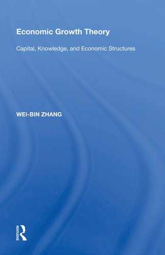
We consider that group 1's propensity to own wealth is higher than group 2's and group 1 works more effectively than group 2. Group 1's population is less than group 2's population. We assume that the income transfer rate is 10 percent. Figure 5.1 shows behavior of the national aggregated variables. Figure 5.1a shows that the national wealth, the national consumption, and the total output rise. As demonstrated in Figure 5.1b, the rate of interest rises and the wage rates of the two groups rise as time passes. Figure 5.2 depicts the motion of the individual incomes and consumption. We see that both the current income and consumption per worker rise as time passes.

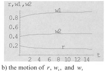
Figure 5.1 Behavior of the Aggregated Variables


Figure 5.2 The Behavior of the Individual Variables
5.2 Does Inequality Accelerate Growth?
It is recognized that physical capital accumulation and human capital accumulation occur in different processes and by different principles. Physical capital accumulation can be effectively conducted by a small portion of the population (the capitalist class); while human capital accumulation can be effectively conducted by involving almost all the people. They are fundamentally asymmetry. The process of development is marked by an endogenous transition from the domination of physical as a prime engine of economic growth to a gradual increase in the importance of human capital accumulation, knowledge creation, and innovations for the growth progress.21 Income and wealth inequality is conductive for physical capital accumulation whereas equality is conductive for human capital accumulation. In early stages of industrialization as physical capital accumulation is the main source of economic growth, inequality enhances the process of development by channeling resources towards individuals whose marginal propensity to save is higher. In early stages of industrialization physical capital is scarce, the rate of return to physical capital tends to be higher than that of human capital. Under the assumption that the marginal propensity to save is an increasing function of the individual's wealth, inequality increases aggregate savings and capital accumulation. As capital accumulates, the rate of return to human capital rises. As human capital accumulation gradually becomes the prime source of economic growth, equality stimulates investment in human capital investment and promotes economic growth. As wages further increase, the adverse effect of inequality on growth becomes insignificant. According to this view, inequality has a positive relationship with economic growth in early stages of economic development and a negative one in later stages of development. Referring to the contemporary world, we should also mention a case that an economy may emphasize human capital accumulation even in early stages of development. A poor economy may start industrialization with heavy investment both in human capital and physical capital - the former through education and the latter through borrowing (foreign investment) and saving. If inequality has a positive effect on capital accumulation and a negative effect on human capital accumulation, it is possible that inequality will not benefit growth even in an early stage of economic development.
We now examine impact of changes in group l's wealth K1(t) and the income transfer rate φ upon growth rates of some variables. First, we examine the current income Y*(t) (= F(t)). The growth rate of Y(t) is equal to the growth rate of the output, by equation (5.1.1) we have:
Substitution of equations (5.1.5) into the above equation gives:
By equations (5.1.2) and (5.1.3):
By equations (5.2.1) and (5.2.2), we have:
In the short term, strengthening distributional policy accelerates (reduces) the growth rate of the current income if group 2's propensity to own capital is higher (lower) than group 1's, i.e., dgy / dφ >(<) 0 in the case of λ2, > (<) λ1. If income is transferred from the lower propensity to own wealth group to the higher one, the economy's 'aggregated' saving propensity rises. Since we are dealing with a neoclassical growth economy, an increase in the propensity to save leads to higher growth (as in the OSG model). We see that Malthus was right with his argument that altruism would reduce the national growth rate and thus reduces national wealth. If λ2 = λ1, dgY / dφ = 0. If the two groups have an identical preference structure, the distribution policy has no impact on the national economic growth rate. We can thus explicitly judge the direction in effects of change in the distribution policy on the economic growth rate when the sign of difference in the propensities to own wealth (which sometime means, roughly as explained in Chapter 2, the propensity to save in the literature) is known.
If group 2's propensity to own wealth is higher than group 1's, then as group 1 has more wealth, the national growth rate declines, i.e., dgY / dK1 < 0 in the case of λ2 ≥ λ1 In the case of λ2 < λ1, we have ambiguous impact of enlarged wealth gap on the national growth rate. Only if the rich group has a higher propensity to own wealth, it is possible that an increase in wealth of the rich accelerates economic growth. Let us examine a case that group 2's propensity to own wealth is negligible (λ2 ≈ 0). We have:
Observing F = Y1 + Y2, we conclude that dgY/dK1 is positive if group 2 has some wealth and the transfer rate φ is not high. If group 2 has little wealth, then the growth rate falls as group 1 accumulates more wealth.
It is also important to examine the growth rates of the two groups' current incomes as wealth is accumulate or the distributional policy is changed. The rates are given by:
in which:
Differentiation of equations (5.2.3) with respect to φ yields:
in which:
Mathematically, it is straightforward to analyze the effects of changes in any parameter on growth rates of the variables in the system. We omit analysis because we can provide little new insights from complicated expressions.
We now demonstrate possible effects of φ upon dynamics of the system. Except φ, we still specify the parameter values as in (5.1.6). We increase φ from 0.1 to 0.25. Figures 5.3 and 5.4 describe the impact. The solid lines depict the variable values corresponding to φ — 0.1; while the dashing lines to φ = 0.25. As the income transfer rate rises from 0.1 to 0.25, the national income, wealth, and consumption decline, the rate of interest slightly rises and the wage rates of the two groups slightly fall. As demonstrated in Figure 5.4a, as the income transfer rate increased, group 1's current individual income falls and group 2's individual income rises. Figure 5.4b shows that as φ rises, group 1's individual consumption falls and group 2's individual consumption rises.

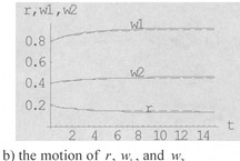
Figure 5.3 The Aggregated Variables Change as φ Rises from 0.1 to 0.25


Figure 5.4 The Group-Related Variables Vary as φ Rises from 0.1 to 0.25
5.3 Properties of the Dynamic System
As all the other variables are uniquely determined as functions of K1(t) and K2(t), it is sufficient to examine dynamic properties of equations (5.1.5). Equilibrium is given as a solution of the following equations:
By equations (5.1.3) and (5.1.2), we get:
where φ0 ≡ 1 - φ. Substituting equations (5.3.2) into equations (5.3.1) yields:
Dividing the first equation in equations (5.3.3) by the second one, we get:
in which δ0 ≡ δ1/δ2 and Λ ≡ K1/K2. The above equation has a unique positive solution:
in which:
From the first equation in equations (5.3.3) and (5.1.1), Λ ≡ K1K2 and Kx1+ K2 = K, we solve Ki1and K2 as follows:
We determine the steady state values of all the variables by the following process: K1 and K2 by equations (5.3.5) -> K1 + K2 = K -> F by equation (5.1.1) -> r and Wj, j = 1,2 by equations (5.1.2) —> Y1 and Y2 by equations (5.1.3) -> Sj, and Cj by equations (5.1.4).
The stability condition is given in Appendix A.5.1. If:
then the equilibrium point is stable. It should be remarked that even the above condition is not satisfied, the equilibrium may be stable.
Proposition 5.2.1
The dynamic system has a unique equilibrium. If (5.3.6) holds, then the equilibrium is stable. In particular, if φ = 0, the unique equilibrium is stable.
Before examining impact of changes in the parameter φ upon the equilibrium, we examine the conditions that the altruist group has higher income than the altruism-receiving group, i.e., y1 > y2 in the steady state. By equations (5.3.1), we get Yj = δjKj. Condition y1, > y2 is guaranteed if δΛ > n is held. Substituting equations (5.3.4) into δΛ > n yields:
Using the definitions of c and b, the above inequality is rewritten as follows:
It is straightforward to see that the denominator is larger than the numerator. Since φ is positive, it is necessary to require the numerator to be positive. It is straightforward to show that if we specify:
y1 > y2 is held at the steady state. In the case of φ = 1 which holds if the two groups have the same preference, the above inequality is rewritten as:
Since the two groups have the identical preference, we see that y1 > y2 can hold only if 1 > z. That is, group l's wage rate is higher than group 2's. For a fixed z (< 1), the above inequality (which guarantees y1 > y2) is held if φ and/or n are/is small.
5.4 The Distribution Policy and the Equilibrium
This section is concerned with impact of changes in φ on the equilibrium of the dynamic system. First, taking derivative of equation (5.3.4) with respect to φ yields:
where we use 2bΛ - c = - Λ2 < 0 and:
The increase in φ reduces the ratio of the capital stock owned by the altruist and the altruism-receiving group.
We examine the ratios of consumption, wealth, and income per capita between the two groups. From Yj = δjKj, we get y1/y2 = δΛ/n. From equations (5.3.1) and (5.1.4), we get:
Taking derivatives of these equations with respect to φ yields:
The ratios of consumption, wealth, and income per capita between the altruist group and the altruism-receiving group are reduced as the altruist group strengthens altruism.
From equations (5.3.5) and K = (1 + Λ)K1/Λ, we obtain:
The capital owned by the altruist group is reduced. Since the comparative static analysis is conducted without specifying any parameter value, we see that the altruist group's wealth is reduced when its altruism is strengthened. We will see in the next section that this may not be true when the altruism-group's working efficiency is related to the altruism. The total capital and group 2's capital may be either increased or decreased. We see that even when group 2's capital is increased, the total capital may be still reduced. It is straightforward to calculate the impact upon the consumption, income and capital per capita of the two groups as follows:
The altruist group's income, consumption, and capital per capita will be reduced as its altruism is strengthened. The impact upon the altruism-receiving group's living conditions is ambiguous. By equations (5.1.2) and (5.1.2), we get:
Since the impact on K is ambiguous, we see that it is necessary to further specify the parameter values in order to get explicit conclusions about the wages and the total output. In the case that K is reduced, the wage rate of each group and the total output are reduced and the interest rate is increased. In sum, we see that as the altruism is strengthened, the national output may be either increased or decreased, the altruism-receiving group's living conditions (in terms of consumption and wealth per capita) may be either improved or deteriorated, the altruist group's living conditions are reduced, and the gaps in living conditions between the two groups are reduced.
Proposition 5.4.1
An increase in φ has the following impact on the steady state values: (i) the altruists' per capita capital, per capita consumption, and per capita income are reduced; (ii) the altruism-receiving group's per capita consumption, and per capita income may be either reduced or increased; and (iii) the national wealth and income may be either increased or decreased.
We now simulate the model to demonstrate how the equilibrium values are affected by change in φ. We specify the parameter values as follows:
As the income transfer rate rises, the equilibrium values of the total output, the wealth, and the consumption fall. Figure 5.5b shows that the wage rates of the two groups fall and the rate of interest rises. As Figure 5.5 demonstrated, the equilibrium values of group l's individual income, wealth, and consumption fall. When the transfer rate is low, the equilibrium values of group 2's individual income, wealth, and consumption rise as φ rises. Nevertheless, when the transfer rate becomes low, the equilibrium values of group 2's per capita wealth and consumption fall as the income transfer rate rises.

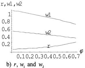
Figure 5.5 The Values of the Aggregated Variables for 0.01 ≤ φ ≤ 0.7


Figure 5.6 The Values of the Individual Variables for 0.01 ≤ φ ≤ 0.7
It is well known that steady state values of per capita variables in the neoclassical growth theory are dependent on the propensity to save. When one group transfers incomes to another group, the 'aggregated savings' behavior would be changed when the two groups have different propensities to save. This change in savings behavior (due to altruism) may result in increases or decreases of the national output and wealth. To illustrate this point, let us consider the case that the two groups have the identical preference, i.e., λ ≡ λ1 = λ2. In this case, adding the two equations in equations (5.3.2) yields Y1 + Y2 = F. Using this relation and adding the two equations in equations (5.3.1), we get F = δ1K. Solving the above equation yields:
(5.4.4)
where we use equations (5.1.2). Using equation (5.4.3) and K2 = K /(1 + Λ), we get:
We thus have the following corollary.
Corollary 5.4.1
Let the two groups have the identical preference. When the altruist group strengthens altruism (i.e., φ being increased), we have the following results: (i) the altruists' per capita capital, per capita consumption, and per capita income are reduced; (ii) the altruism-receiving group's per capita consumption, and per capita income are increased; and (iii) the national wealth and income are not affected.
Since the two groups have the same propensity to save, income transfers between the groups would not affect the 'aggregated savings behavior'. It is reasonable to expect that the total capital will not be affected. The above corollary implies, for instance, that it is possible for a society to equalize its distribution of wealth and income without reducing its total capital and income if there is no taxation.
We now simulate impact of z and λ2, on the equilibrium values. Accepting except for z - (5.4.3) and fixing φ = 0.2, we obtain the effects of change in z for 0.1 ≤ z ≤ 1.5. As group 2's level of human capital rises, the total wealth, income, and consumption increase. As group 2's human capital is improved, group 1's wage rate falls, but group 2's wage rate rises and the rate of interest rises. Group 1's per capita wealth, income, and consumption fall, while group 2's per capita wealth, income, and consumption rise.


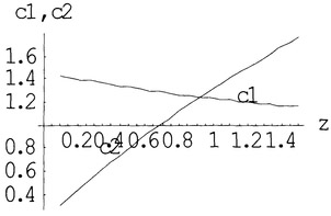
Figure 5.7 The Equilibrium Values for 0.2 ≤ z ≤ 1.5
Accepting - except for λ2 - (5.4.3) and fixing φ = 0.2, we obtain the effects of change in λ2, for 0.05 ≤ λ2 0.85 as in Figure 5.8. As group 2's propensity to own wealth increases, the total consumption and wealth rise but the output is only slightly changed. The wage rates of the two groups become lower and the rate of interest is slight increased. As consequences of decline in group 2's propensity to own wealth, group 1's individual income, wealth, and consumption all fall. Group 2's individual wealth is increased but the group's current income is only slightly changed. When the group's propensity to own wealth is low, group 2's per worker consumes more as λ2, rises.


Figure 5.8 The Equilibrium Values for 0.05 ≤ λ2 ≤ 0.85
We now examine effects of group 2's population on the equilibrium structure. Accepting - except for N2 - (5.4.3) and fixing φ = 0.2, we obtain the effects of change in N2 for 0.01 ≤ N2 ≤ 20 as in Figure 5.9. As group 2's population grows, the total capital and output rise, and the total consumption declines. The two groups' wage rates fall and the rate of interest rises. We see that as the poor and less educated group's population rise, any group's individual wealth, income, and consumption fall. In particular, we observe that if group 2's population is small, even with a low transfer rate, the consumer of group 2 can enjoy higher consumption level than the consumer of group 1.
5.5 Human Capital and the Distribution Policy
The previous section examined the impact of changes in the parameter φ on the economic system. We showed that if the altruism-receiving group does not change its preference and the group's human capital is not affected by changes in φ, then the altruist group would not economically benefit from giving money to the other group. We assumed that altruism has no impact on other aspects of the society except upon the endogenous variables. But it may be argued that altruism may affect some aspects of the society which are not taken into account so far. Possible influences of altruism are also dependent on the way in which wealth and income are spent. For instance, when the poor receives money from the rich, economic conditions would be different, depending on whether the poor spends the received money on education or eating. As mentioned by Keynes, if some labor force is unemployed, then monetary transfers from the rich to the poor would economically benefit the rich as well. Since we assume the full employment of labor force, to provide insights into the economic mechanism by Keynes, we may consider a case that the monetary transfer from the rich to the poor would increase the poor group's working efficiency. We now examine what will happen to the two groups' living conditions when the altruism-receiving group changes its work efficiency after receiving altruist contributions from the other group.


Figure 5.9 The Equilibrium Values for 0.01 ≤ N2 ≤ 20
In this section, we consider a possible case that the altruism-receiving group's human capital is related to the income transfer rate from the altruist group. We assume z = z0φm. z0 > 0 and 1 > φ > 0. We are concerned with the impact of changes in φ on the system when m is taken on different values. It should be remarked that the previous section is a special case of this section with m = 0. If m > 0, it means that the altruism-receiving group will improve its human capital when the altruist group strengthens its altruism. The condition m < 0 means that the altruism-receiving group works less effectively when the altruist group strengthens its altruism. It is important to examine what will happen to the system when the altruism-receiving group reacts to altruism in different ways.
Taking derivatives of equations (5.3.4) with respect to φ yields:
where Λ* < 0 is defined as in equations (5.4.1) and z* ≡ dz/dφ = dφ = mz/φ. We see that if m > 0, then A is decreased as φ increases. Since m > 0 implies that as group 2 receives more money from group 1, group 2 increases its working efficiency, it is reasonable to see that the capital ratio between the two groups is reduced when φ is increased. If m < 0, the sign of dΛ/dφ is ambiguous. This means that if the income and wealth redistribution makes the altruism-receiving group to invest less in human capital and work less effectively, it is possible that the gap between the two groups' wealth is enlarged when altruism becomes stronger in society.
We have:
In the case m ≥ 0, the ratios of consumption, wealth, and income per capita between the altruist and altruism-receiving group are reduced as the first group strengthens altruism. In the case of m < 0, the impact is ambiguous.
From equations (5.3.5) and K = (1 + Λ)K1 / Λ, we obtain:
where K*1, K*2 and K* are defined in equations (5.4.2). In the remainder of this section, we require:
Since we required Λ / n > 1 / δ > 1 (which we discussed in examining the condition for y1 > y2 in Section 3), we see that the above requirement is not strict.
In the case m < 0, the capital owned by the altruist group is reduced. The total capital and group 2's capital may be either increased or decreased. In the case m > 0, it is possible that K1 K2 and K are increased as φ is increased. This means that if the altruism increases the altruism-receiving group's incentive to accumulate human capital, even the altruist group's capital may be increased. Everyone can economically benefit from the altruism.
It is straightforward to calculate the impact upon the consumption, income and capital per capita of the two groups as follows:
By equations (5.1.2) and (5.1.2), we get:
If the altruism-accepting group increases its human capital when altruism is strengthened, then everyone in the society may economically benefit. We now try to identify such a case (with m > 0).
Let us consider the case that the two groups have the identical preference, i.e., λ ≡ λ1 = λ2 and ν = ν2. In this case, we have δ = 1, Y1, + Y2 = F, and K is given by equation (5.4.3). Using equation (5.4.3):
we get:
We thus have the following corollary.
Corollary 5.5.1
Let the two groups have the identical preference and m > 0. When the altruist group strengthens altruism (i.e., φ being increased), we have the following results: (i) the altruists' per capita capital, per capita consumption, and per capita income may be either increased or reduced; (ii) the altruism-receiving group's per capita consumption, and per capita income are increased; and (iii) the national wealth and income are increased.
It should be noted that if m < 0 (which may be interpreted as Malthus' assumption), the national wealth and the altruist group's wealth are definitely reduced. If the reduction in the altruism-receiving group's productivity is so high that Λ is increased, then we conclude that the altruism-receiving group's per capita consumption and wealth are reduced. In other words, Malthus' view that no one would benefit from strengthening altruism is justified.
By the way, there are different viewpoints about man's nature and interrelations between beliefs and action.22 It is argued that altruism may not be a preexisting 'stock' as we assumed. For instance, Aristotle held that virtues are neither innate nor contrary to nature. But from the sustainable point of view, altruism may be conducted in large scales in the long term only when altruism has positive consequences not only for the altruism-receiving groups but also for the altruist groups. As far as society as a whole is concerned, it seems important to find out what kinds of altruist behavior would promote welfare of different individuals and increase productivity of the society.
It is well known that Adam Smith advocated that the government should intervene education in market economy so that all the social groups of the people would benefit from economic development. In our modeling framework Smith's idea may be interpreted as that 'altruism' would benefit all the groups if it were targeting at improving human capital through spreading education. Our analysis may also provide insights into Malthus' viewpoint that altruist may neither benefit the poor nor enrich the rich. Keynes' viewpoint about government's redistribution policy and economic growth is a proper example that 'social altruism' is in harmony with economic development and economic benefits of the different groups. It may be held that our analytical results provide insights into the viewpoints held by Smith, Malthus, and Keynes. Alfred Marshall holds:23 'The supreme aim of the economist is to discover how this latent asset [being capable of more unselfish service than they generally render] can be developed more quickly and turned to account more wisely.' Our simple model shows that there is no unique correspondence between altruism and economic consequences. In other words, altruism may either cause economic benefits or loss to the altruist group as well as to the altruism-receiving group.
5.6 Dynamics of the Loren Curve and the Kuznets Curve
We can find the two opposite viewpoints about the relationship between economic growth and income/wealth distribution. Kuznets proposed his famous hypothesis that inequality first rises - the period of trickle-down growth (which means that inequality is narrowed as wealth accumulates) and eventually falls in the development process of an economy.24 Recent history of economic development has not confirmed this hypothesis - recent empirical studies indicated a fairly robust negative impact of income inequality on the growth rate of national income in cross-country studies.25 No inclusive conclusions have been empirically found about relationship between distribution and growth. Even in the same stage of economic development, relationship may be either positive or negative, depending on cultural, institutional, and political factors. As mentioned by Grossmann, the rate of economic growth may be negatively related to inequality by the following reasons. In the fiscal policy approach, it is assumed that higher inequality would lead to more redistribution and redistribution would slow down the economic growth. The imperfect capital markets approach holds that imperfect capital markets would depress growth. The sociopolitical instability approach asserts that higher inequality leads to political or social instability, creating a harmful environment for economic growth. The fertility approach makes a hypothesis that higher inequality should increase fertility rates and reduce human capital investment.
Kuznets was concerned with dynamic interaction between the personal income distribution and economic growth.26 The Kuznets curve describes an inverted U-shaped relationship between the development of an economy and income inequality. According to the Kuznets hypothesis, in a poor economy like China income inequality tends to be enlarged as growth increases; while in a rich economy like Japan income inequality tends to be narrowed if growth is sustained. Kuznets held that in earlier development, rapid industrialization and urbanization would enlarge income inequality. In the situation that income is more equal among the rural population than the urban population and the rural population is poorer than the urban population on average, the rural population tends to become poorer as urbanization is deepened. The difference is also strengthen since productivity growth would not be slower in urban than in rural areas. Nevertheless, he argued that the inequality would eventually not be widened because, for instance, descents of talented individuals with high incomes are not necessarily able to have high earnings, mature urban areas would provide a better basis for securing greater income shares, and there should an increasing demand for redistribution in democratic societies as the economy grows. He also recognized that the marginal propensity to save is an increasing function in income which would tend to increase both wealth and income inequality with growth of the economy.
We now consider the case where the population is composed of two pure worker and capitalist - classes like in traditional Marxian economics. At the time that Ricardo wrote, the factor distribution was considered as directly relevant to the personal distribution, mainly because each kind of source could be properly identified with the class that owned that source. Workers make up a fixed fraction nw of the population and capitalists, 1 - nw. Workers supply labor but don't own any capital stock; capitalists own all the capital stocks but don't work. Then, according to the marginal conditions, the relative distribution of incomes in the population depends only on the share of labor and of capital. The Cobb-Douglas production function implies that the capitalists' and workers' shares are respectively equal to α and 1 - α in the total income.
We now draw the Lorenz curve for this two-class economy. Arranging the individuals in ascending order according to their incomes from the poorest to the richest, the Lorenz curve plots the proportion of people against the corresponding proportion of total income obtained by those people. In the case of the two classes (supposed that the worker class is poor), the worker class has 1 - α of the total income, while the capitalist has the rest. In general, consider that there are N individuals, whose incomes are denoted by yi, i = 1,..., N, with y1 < y2 ... < yN. The Lorenz curve shows diagrammatically the relationship between the proportion of people (equaling k/N) with income less than or equal to a specified amount (the k(t) th income in the list), and the proportion (expressed as ) of total income obtained by those individuals. Typically the Loren curve lies below the diagonal line except when k equals N. The extreme case of inequality is where everyone has nothing, except one person. The Loren curve follows the bottom and right-hand edge of the box. If everyone has the same income, the Loren curve in this case of complete equality is the diagonal line. Any distribution having a Lorenz curve that is closer to the diagonal of equal incomes than another distribution over the whole range is said to be more equal. Another important indicator for measuring the overall extent of inequality is the Gini coefficient, which is the ratio of the area between the Lorenz curve and the diagonal line to the maximum such area.
The Lorenz curve for the two-class economy is given by Figure 5.10. The slope of the first segment is equal to 1 - α divided by nw; the slope of the second segment is equal a to divided by 1 - nw. A rise in the income share moves the Lorenz curve upwards and closer to the line of equal incomes.
Today, the Ricardian classification is scarcely adequate. Most of the population both earns wages by working and accumulates wealth through saving. We now define ratios of the economic variables between the two groups:
First, we examine dynamics of these ratios and then make comparative static analysis with respect to some parameters, based on the calculation results in the preceding sections. Corresponding to Figures 5.1 and 5.2 (under (5.1.6)), we depict the motions of these ratios by Figure 5.11.

Figure 5.10 The Lorenz Curve for the Worker-Capitalist Economy


Figure 5.11 The Dynamics of the Lorenz Curve in the Two Group Model
Corresponding to Figures 5.1 and 5.2, we demonstrate the effects of φ upon dynamics of the ratios. Except φ, we still specify the parameter values as in (5.1.6). We increase φ from 0.1 to 0.25. Figure 5.12 portrays the impact. The solid lines depict the variable values corresponding to φ = 0.1; while the dashing lines to φ = 0.25. The distributional policy has a strong impact on the distribution of individual wealth and income. As φ rises, the distributional ratios between the two groups as well as the individuals of the two groups are 'improved'.
We now simulate the model to demonstrate how the equilibrium values of the ratios are affected by change in φ. Corresponding to Figures 5.5 and 5.6, we illustrate the impact as in Figure 13. As φ rises, as already demonstrated in the dynamic case, the distribution between the two groups is 'improved'.


Figure 5.12 The Distributional Ratios Change as φ Rises from 0.1 to 0.25


Figure 5.13 The Equilibrium Values of the Ratios for 0.01 ≤ φ ≤ 0.7
Corresponding to Figure 5.7, we illustrate the impact of change in group 2's level of human capital as in Figure 5.14. As the level of human capital is increased, group 2's comparative conditions are improved. As group 2 has the same level of human capital as that of group 1, the per capita consumption and income of group 1 are higher than the per capita consumption and income of group 2.


Figure 5.14 The Equilibrium Values of the Ratios for 0.1 ≤ z ≤ 1.5
The effects of change in group 2's propensity to own wealth on the ratios are given in Figure 5.15. In correspondence to Figure 5.8, we see that as λ2 rises, the ratios of the total income, the total wealth, and the wealth per capita, and per capita income are increased.
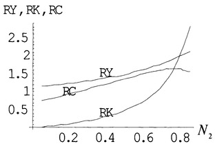

Figure 5.15 The Equilibrium Values of the Ratios for 0.05 ≤ λ2, ≤ 0.85
Corresponding to Figure 5.9, we illustrate the effects of N2 on the ratios as in Figure 5.16. As group 2's population rises, the ratios of group 2's and 1's total incomes, wealth, and consumption increase, but the ratios of group 2's and 1's individual incomes, wealth, and consumption fall.


Figure 5.16 The Equilibrium Values of the Ratios for 0.01 ≤ N2 ≤ 20
5.7 Endogenous Time in the Two-Group Model
This section introduce endogenous time into the two-group model proposed in this chapter. We are concerned with a one-sector and two-group growth model with endogenous savings and time distribution. We examine a dynamic interdependence of two groups with different productivity and preferences under perfect competition, omitting income transfers between groups. The model proposed here is a combination of the OSG model with endogenous time in Section 4.4 and the two-group model in Section 5.1.
Except time the production aspects of the economic system under consideration are similar to the one-sector growth model. The variables F(t), r(t), Nj, Kj(t), Cj(7), Sj(t), wj(t) are defined as before. Let Tj(t) and Thj(t) stand for respectively the working time and leisure time of each member of group j. We assume that the labor and capital are always fully employed. The total capital stock K(t) and the total qualified labor force N* are given by K1 + K2 = K and N* = T1N1 + zT2N2, where z is defined as before and TjNj is the total working time of group j at time t. Here, we omit any other possible impact of working time on productivity. For instance, if over-working reduces productivity per unity of working time, it is much more complicated to model the qualified labor force and working time. The parameter z distinguishes the difference in productivity of the two groups. With group 1's human capital as the basis of measurement, the terms, T1N1 and zT2N2, are respectively the qualified labor force of groups 1 and 2. Here, we neglect the possible impact of education, training and other costly learning efforts on human capital. The production function of the economy is specified as F(t) = K(t)αN*(t)β.
The marginal conditions are given by:
The current income Yj(t) of each group consists of its wage income wjTjNj and payment rKj of interest for its capital. The net incomes are given by:
The utility level Uj(t) of group j is given by:
where σj, and λj are respectively group j's propensities to use leisure time, to consume and to own wealth. The budget constraints are:
Let T0 denote the total available time (which is assumed to be equal between the two groups). The time constraint requires that the amounts of time allocated to each specific use add up to the time available Tj + Thj; = T0, j = 1, 2.
Substituting these equations into equations (5.7.2) yields:
where: Ŷj(t) ≡ r(t)Kj(t) + wj(t)T0Nj + δKj (t), j = 1, 2.
Maximizing Uj subject to the above budget constraints yields:
where:
According to the definitions of Sj group j's capital accumulation is:
We have:
We have thus built the dynamic model. The dynamics consist of two dimensional differential equations for K1(t) and K2(t). In order to analyze the properties of the dynamic system, it is necessary to express the dynamics in terms of the two variables at any point of time. From equations (5.7.4) and the definitions of Ωj(t) we see that it is sufficient to express Tj(t) as functions of K1(t) and K2(t).
Proposition 5.7.1
The dynamics are given by the following two-dimensional system:
where Ωj(K1,K2) are functions only of K1 and K2. All the other variables are uniquely determined as functions of K1(t) and K2(t) at any point of time.
The above proposition is proved b Zhang.27 The system (5.7.5) determines the motion of K1(t) and K2(t). As all the other variables are uniquely determined as functions of K1(t) and K2(t), it is sufficient to examine the dynamic properties of equations (5.7.5). Equilibrium is given as a solution of the following equations:
In Appendix 5.2 in Zhang just referred, it is proved that the ratio Λ ≡ K1 K2 of the capital stocks owned by groups 1 and 2 is determined by the following equation:
in which:
We may rewrite equation (5.7.7) as:
where:
Proposition 5.7.2
The dynamic system has a unique equilibrium. The unique equilibrium value of Λ is determined by:
All the other variables are given by:
→ K1 + K2 = K → F(t) = KαN*β —> r and wj. by equations (5.7.1) -> Yj = rKj, + wjTjNj —> Cj and Sj. by equations (5.7.3).
The above proposition is proved in Appendix 5.2 in Zhang. At equilibrium, we have
These ratios are important for comparing the living conditions of the two groups.
From equation (5.7.7), we see that it is generally difficult to judge whether Λ ≥ 1 or Λ < 1. To explain the impact of differences in the preference and productivities of the two groups, some special cases are investigated. For convenience, in the remainder of this section it is assumed that the population of the two groups is equal, i.e., N1, = N2.
Let us examine the case of λ1, = λ2, and σ1, = σ2, z > 1 when the two groups have the identical preference and group 1 is less productive than group 2. From equation (5.7.7), Λ is given by: Λ = 1/z. From this equation and equation (5.7.8), we have:
Group 1 owns less capital, has lower net income, and consumes less goods than group 2, but their working time is the same at the equilibrium.
In the case of λ1 < λ2, ξ1, = ξ2 and σ1, = σ2, z = 1 when group 1's propensity to hold wealth is lower than that of group 2 and all other characters of the two groups are identical, from equation (5.7.7), we know:
where:
It is straightforward to check:
In this case, group 1 owns less capital, has lower net income, consumes more goods and works shorter time than group 2.
In the case of λ1, = λ2, ξ1, = ξ2, and σ1 > σ2, z = 1 when group 1's propensity to use leisure time is higher than that of group 2 and all the other characters of the two groups are identical, by equation (5.7.7) we get:
Group 1 spends longer time at home, owns less capital, and has lower net income and lower consumption level than group 2.
The three cases are intuitively acceptable. These cases illustrate the impact of groups' differences in the preferences and productivity on the differences in the living conditions and wealth. As the solutions have been explicitly given, it is quite easy to examine other possible combinations of the preference parameters.
5.8 The OSG Model with Multiple Consumers
This chapter developed a growth model with two types of consumers. We now extend this framework to include many types of consumers. Let there be n (or types of) consumers, indexed by j, in the economy. Each type of consumers has a fixed number of the population, denoted by Nj. Since there is a single production sector in the economy and labor is always fully employed, we are concerned with an aggregated labor force N(t):
where zj(t) and Tj (t) are respectively the level of human capital and work time of group j, j = 1,..., n.
Production is described as combination of labor and capital. Time is represented continuously by a numerical variable which takes on all values from zero onwards (t ≥ 0). Let K(t) denote the total capital stock existing at each time t. Capital is malleable in the sense that one need distinguish neither its previous use nor the factor productions of its previous use. Like before, the production process is described by some sufficiently smooth function F(t) = F(K(t),N(t),t). Here, the time variable stands for possible exogenous technological change. We assume that the production function F(K(t),N(t),t) is neoclassical. The marginal conditions are r(t) = Fk(t) and wj(t) - zj(t)FN (t), where r(t) is the rate of interest and wj(t) stands for group j's wage rate per unity of work time.
Let Kj(t) and Yj(t) be the capital stocks owned by and the current income level of group j. The total capital K(t) and total current income Y(t) are:
We introduce two vectors to measure the structures of income and wealth distribution:
We now describe behavior of consumers. Utility function of group j is:
where Thj(t), Cj(t), and Sj(t) respectively stand for leisure time, consumption and savings of group j (which are consumers'decision variables). Variables K̄(t), Ȳ(t), and t are factors that may affect preference structures of consumers. For instance, we may use t to express ages of consumers. We thus can deal with behavior of different age groups by considering their typical behavior. For retired people, the work time is simply equal to zero and they consume their wealth or live on government's benefit policy or their children' 'altruism' or filial piety.
The current income Yj(t) of group j consists of the wage income and payment interest for its capital, i.e.:
We know .
The gross disposable income of group j is:
As in Chapter 2, the budget constraint is:
The time constraint requires that the amounts of time allocated to each specific use add up to the time available Tj(t) + Thj(t) = T0. Substituting this equation into the above budget constrain yields:
(5.8.1)
where:
The consumer is to choose his most preferred bundle (Thj(t), Cj(t), Sj(t)) of consumption and saving under his budget constraint. The utility maximizing problem at any time is defined by:
(5.8.2)
The conditions for existence of optimal solutions for the above problem can be found in advanced textbooks on microeconomics.28 We denote an optimal solution as function of the disposable income and the other variables:
(5.8.3)
where X(t) ≡ (K̄(t)T,Ȳ(t)T,t). Capital accumulation follows:
As Ŷj(t) and X(t) are functions of K̄(t) and t at each moment, the above equations are rewritten as:
These n -dimensional differential equations determine the dynamics of all the variables at any point of time. Hence, solving the system (5.8.4) determines value of any variable in the system in any time. It can be seen that the two models developed before in this chapter are special cases of this general model.
5.9 Simulating the Three-Groups OSG Model
This section simulates the OSG model of three groups with the Cobb-Douglas production and utility functions. For simplicity, we fix time distribution. The variables are defined as in the previous section with n = 3. The aggregated labor force N* is:
where zj is the level of human capital of group j, j = 1, 2, 3. The production function and marginal conditions are:
where A is the total productivity, r(t) is the rate of interest, and wj (7) stands for group j's wage rate per unity of work time. Let Kj(t) and Yj (t) be the capital stocks owned by and the current income level of group j. The total capital K(t) and total current income Y(t) are:
As in Section 5.8.1, the consumers' behavior are described by:
where:
Substituting Sj(t) into K̇j(t) = Sj(t) - Kj(t) yields:
where δj ≡ ξj / λj + δk. We now simulate the model. We specify the groups' human capital and preferences as follows:
Group 1 is the rich class - with the highest level of human capital and highest propensity to own wealth. The population share of the rich in the total population is only 1/16 percent. Group 2 is the middle class - with the middle level of human capital and 'middle propensity' to own wealth. The population of this group is 5/16 percent. Group 3 has the lowest level of human capital and the lowest propensity to own wealth. This group has the largest share in the total population. We specify the rest parameters as follows α = 0.25, A = 1.3 and δk = 0.05.
The motion of the total income, consumption, wealth, the wage rates, the rate of interest, the individual incomes, and individual consumption levels are illustrated as in Figure 5.17. As for the two-group model, we can simulate the motion of the model with varied values of parameters.


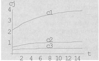
Figure 5.17 The Time-Dependent Paths of the Key Variables
5.10 The OSG Model with Sexual Division of Labor
This section is concerned with another type of economic evolution with group differences. Different from the previous sections, we classify population into two groups based on gender. For simplicity, we are only concerned with an ideal - a very simple case - when each woman has only one husband and every adult must be married.
Dynamic interactions between economic growth and sexual division of labor and consumption have caused attention of economists. Yet there are only a few theoretical economic models which explicitly take account of these interactions within a compact framework. Over the years there have been a number of attempts to modify the neoclassical consumer theory to deal with economic issues about endogenous labor supply, family structure, working hours and the valuation of traveling time.29 It has been argued that the increasing returns from human capital accumulation represent a powerful force creating a division of labor in the allocation of time between the male and female population.30 There are studies on the relationship between economic growth and the family distribution of income.31 There are studies of the female labor supply. Women choose levels of market time on the basis of wage rates and incomes. Lifetime variations in costs and opportunities - due to children, unemployment of the spouse, and general business cycle variations - influence the timing of female labor participation.32 There are studies on the relationship between home production and non-home production and time distribution. Possible sexual discrimination in labor markets has attracted much attention from economists.33 The gains from marriage may be reduced as people become rich and educated. The growth in the female population's earning power may raise the forgone value of their time spent at child care, education and other household activities, which may reduce the demand for children and encourage a substitution away from parental activities. Divorce rates, fertility, and labor participation rates may interact in much more complicated ways. Decision making about on family size is extremely complicated.34 Irrespective of numerous studies on the complexity of the family as a subsystem of economic production, family economics - swept into a pile labeled economic demography or labor economics - is often relegated to a somewhat obscure corner of the mainstream studies of economic growth and development.
In Chapter 2, we extended the one-sector growth model to include time distribution and home capital. This section synthesizes these two growth models with home capital and time distribution into a single framework with the dynamic interdependence of sexual division of labor and consumption.35 We consider an economic system similarly to the one-sector growth model proposed in Chapter 2. We assume the same family structure. Each family consists of four members - father, mother, son, and daughter. The total population is equal to 4N. There is division of labor in the family. The children consume goods and accumulate knowledge through education. The parents have to do home work and find job for the family's living. The father and mother may either do home work or do business. The working time of the father and the mother may be different. We assume that working time of the two adults is determined by maximizing the family's utility junction subject to the family and the available time constraints. We omit any possibility of divorce. We assume that the young people get educated before they get married and join labor market and the husband and the wife pass away at the same time. When the parents pass away, the son and the daughter respectively find their marriage partner and get married. The property left by the parents is shared equally by the two children. The children are educated so that they have the same level of human capital as their parents when they get married. When a new family is formed, the young couple joins the labor market and has the two children. As all the families are identical, the family structure is invariant over time under these assumptions.
We assume that labor markets are perfectly competitive. The total labor input N*(t) at time t is defined by N* = N1, + N2 and Nj = zjTjN, where T1(t) and T2(t) are respectively the husband's and the wife's working time and z1, and z2, are the levels of human capital at work of the husband and the wife, respectively. We specify production function of the economy:
where F(t) is the output level at time t, Ki(t) is the level of capital input, and a and β are parameters. The marginal conditions are given by:
where r(t) is the rate of interest and w1(t) and w2(t) are respectively the wage rates per unity of working time of the husband and the wife. From equation (5.10.1), the ratio of the wage rates per unity of time between the husband and the wife is given by w1(t)/w2(t)=z1/z2. The ratio is independent of capital stock and production scale and only dependent on the ratio of human capital. If z1/z2 = 1, the husband and the wife have the identical wage rate per unity of time. The current income Y(t) of each family consists of the wage incomes and the interest payment for the family's capital. The current income at any point of time is given by:
Let us denote T0the husband's and the wife's total available time. The total available working time for any sex is distributed between leisure time and working time. The time constraint requires that the amounts of time allocated to each specific use add up to the time available:
where Thl(t) and Th2(t) are the husband's and the wife's leisure time, respectively. We assume that the family's utility level is dependent on the husband's leisure time, Th1 (t), the wife's leisure time, Th2(t), the level of consumption, C(t), home capital, Kh(t), and the family's net wealth. We specify a typical family's utility function as follows:
in which σ1, σ2, ξ, η and λ are positive parameters. We call σ1, σ2, ξ, η and λ, respectively, the family's propensities to use the husband's leisure time, to use the wife's leisure time, to consume goods, to utilize endurable goods, and to hold wealth. Each family makes decision on the 7 variables, Tj(t), Thj(t), (j = 1, 2), Kh(t), C(t), and S(t) at any point of time.
Since a family consists of several members and each member has his/her own utility function, the family's behavior should be analyzed as the result of all members' rational decisions. The collective utility function should be analyzed within a framework which explicitly takes accounts of interactions within the family's members.36 We simplify these issues by assuming the existence of a family utility function.
The gross disposable income is Y*(t) ≡ Y(t) + K(t). The financial budget constraint is given by:
Substituting Tj(t) + Thj(t) = T0 into the above constrain, we get:
where Ŷ(t) = r(t)K(t) + w1,(t)T0N + w2(t)T0N + δK(t) and δ ≡ 1 — δk.
Each family maximizes U(t) subject to the above budget constraint. The optimal problem has the following unique solution:
where:
Substituting S in equations (5.10.2) into the capital accumulation equation K = S - K yields:
The condition that the total capital stocks K is fully employed at each point of time is expressed by Ki(t) + Kh(t) = K(t).
We have thus built the model. The system has 16 variables, K, Ki, Kh, N*, F, Y, C, S, U, R, Wj, Thj, and Tj (j = 1, 2). It contains the same number of independent equations. We now examine properties of the dynamic system.
First, substituting:
and the marginal conditions (5.10.1) into the definition of Ŷ, we get:
As:
we have:
Substituting C = ρξŶ and S = ρλŶ in equations (5.10.2) into the above equation yields:
Substituting r and wj in equations (5.10.1) into:
we get:
where z ≡ z1 + z2. By this equation and equation (5.10.4):
where:
By Kh = ρηŶ/r in equations (5.10.2) and r = αF / Ki in equations (5.10.1), we have Ŷ = αKhF/ρηKi By this equation, equation (5.10.4) and Kh = K - Ki, we obtain:
where:
Substituting equation (5.10.6) into equation (5.10.5) yields:
It is straightforward to check:
The equation Φ(Ki) = 0 has a unique solution in the interval of:
This implies that for any given positive K(t) at any point of time Ki(t) is uniquely determined as a function of K(t). Summarizing the above discussion, we have the following lemma.
Lemma 5.10.1
For any given positive K(t) at any point of time, the other variables in the system are uniquely determined as functions of K(t) by the following procedure: Ki by equation (5.10.7) → Kh = K - K, -> N* by equation (5.10.6) → F = Kα1N*β -> r, wj j = 1, 2, by equations (5.10.1) → Ŷ by equation (5.10.4) -> C, S and Tj by equations (5.10.2) -> Thj = T0 - Tj.
By the above lemma and equation (5.10.3), we conclude that the dynamics of the system are given by the following differential equation:
in which Ŷ(K) is a unique function of K. From equation (5.10.9), we determine K(t) at each point of time. Then, by Lemma 5.10.1 we solve the values of the other variables in the system at any point of time.
In equilibrium, ρλŶ = K. From the equilibrium equation and Ŷ = αKhF/ρηKi, we solve:
Substituting equation (5.10.6) into this equation and using Kh = K - Ki we obtain:
where:
Substituting Ki in equations (5.10.10) into equation (5.10.7) yields:
Equation (5.10.11) gives a unique equilibrium value of K. By Lemma 3.1, we directly determine the unique equilibrium values of the other variables. To determine stability, we take derivatives of the left-side of equation (5.10.9) to get:
in which we use equation (5.10.4), F = Kα1 N*β and:
which ∂Φ/∂Ki > 0 is given by equations (5.10.8), and equations (5.10.7) and (5.10.6) are used. As we explicitly solved the equilibrium values of the variables, it is easy to calculate the left-hand side of (5.10.12). Summarizing the above discussion, we obtain the following proposition.
Proposition 5.10.1
The dynamic system has a unique equilibrium. The equilibrium is stable (unstable) if the left-hand side of (5.10.12) is negative (positive).
We now examine how the equilibrium values of variables are related to parameters. First, we examine how woman's human capital level affects the time distribution of the husband and wife. With z2 to change, we specify the other parameters as follows:
Figure 5.18 shows how man and woman's working hours vary as woman's human capital changes. For the fixed preferences, from Figure 5.18a we observe that as woman's human capital rises for z2 ∈ [0.5, 0.9], man's working time declines and woman's working time rises. Their working hours become equal only when the wife accumulates more human capital than the husband because we have assumed that the wife makes more contributions to family life than the husband if they spend the same hours at home. Figure 5.18b shows that as woman's human capital rises, her wage rate increases.
We now examine the impact of woman's propensity to stay at home on the equilibrium. Except σ2 and z2, we specify the parameters as in (5.10.13). Let z2 = 0.6 and σ2vary within oσ e∈[0.2, 0.6] As woman increasingly prefers staying at home, woman's work time declines but man's work time increases. As demonstrated in Figure 5.19b, both man and woman's wage rates decline as woman's preference to stay at home becomes stronger.

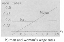
Figure 5.18 The Impact of Woman's Human Capital

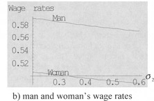
Figure 5.19 The Impact of Woman's Propensity to Stay at Home
Combining Figures 5.18 and 5.19, we illustrate how man and woman's working hours vary with σ2 and z2. We observe that even when man's human capital and time preference remain invariant, man's working hours vary as woman's human capital and time preference change.

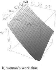
Figure 5.20 The Work Hours and σ2 and z2
5.11 On Modeling Group Differences
The models in this chapter are based on a linear form of qualified labor force given by: N1 + zN2. This form implies a perfect substitution between the two groups. This description is oversimplified if we consider that one group is unskilled and the other is skilled. We now mention a few other directions in aggregating labor force.
First, let us consider a case that human capital is changeable. If we use the same formation of aggregating labor input, a general description of N*(t) should be given by:
where zj (t) are group j's level of human capital at time t. People learn through different sources. They may improve skills by producing. Learning by doing is a source of skill or knowledge accumulation. Schools and universities are established to improve human capital. Through formal education, people learn more about the Nature, man and society. Another possible source of learning, which has not been introduced into formal growth theory, is learning by playing. In different stages of economic development, people learn different things in leisure activities. Clubs and parties not only connect people but also enable men to skillfully manage situations. Readings in leisure are obvious sources of information and knowledge. Sports merely for fun can improve skills for jobs. It is reasonable to assume that zj(t) changes, for instance, according to the following rule (specified in Chapter 8):
żj = learning by doing + learning by education + learning by leisure - the depreciation.
Specifying how learning by doing (or producing), learning by education, learning by leisure, and depreciation are affected by the consumer's resource distributions, we treat z an endogenous variable. If we use the general specification N* = z1N1 + z2N2, we know w1/w2 = z1/z2. The group whose human capital rises mostly rapidly also receives the mostly rapid increase in rewards. Different technological progresses have varied implications of wage differences. Variation in technological change shows up variation in rates of growth of wages.
It can be seen that the wage-ratio between the two groups is totally determined by the effort or human-capital ratio between the two groups. This formation has limitations, for instance, in explaining discrimination in labor market.
To take account of substitution of workers with different skills, introduce another way to generalize N*(t):
where we characterize evolution of human capital or technological change in terms of two functions of time. The variable, zj(t), which may be either exogenous or endogenous, augments the services of group j. It can be shown that the wage ratio is given by:
If we nest N*(t) and K(t) in the Cobb-Douglas production function, the parameter o determines the elasticity of substitution between the two groups in the economy. In Appendix A.5.3, we prove that the elasticity of substitution between the two groups of labor is dependent on the value of the parameter σ:
(5.11.1)
Appendix
A.5.1 Stability Conditions in Section 5.3
Using equations (5.3.2) and (5.1.5), we calculate the Jacobian as follows:
where:
where kj ≡ Kj / K, f ≡ F/K, n1 ≡ N1/N* and n2 ≡ N2/N*.
Substituting (5.3.3) into the above equations for a11 and a22 yields:
The two eigenvalues, ϕj, 1, 2, are given by:
Since a11 < 0 and a22 < 0, the real parts of the two eigenvalues are negative if:
From (5.A.3.2) and (5.A.3.1), we obtain:
where:
in which we use Λ = k1 / k2. We see that if z0 > 0, then z > 0. As the sign of z0 is the same as that of:
We see that if the term is nonnegative, the equilibrium point is stable.
We now show that the equilibrium is stable when φ = 0. Here, we prove the result for a general production function F. We only require that F is neoclassical. It is direct to show that in this case the system is given by:
The dynamic system has a unique equilibrium. At equilibrium we have:
where:
Similarly, we have:
where b2 ≡ βλ2zN2/Q > 0 and z2 ≡ b2 + αλ2k2 > 0. We also have:
The characteristic equation is:
As a11 + a22 < 0, the equilibrium point is stable if a11a22 - a12a21 > 0. We see:
where we use Λ < 0. We thus conclude that the equilibrium point is asymptotically stable.
1 Okun (1975).
2 Atkinson and Bourguignon (2000: 5).
3 Atkinson and Bourguignon (2000: 2). Sahota (1978) provides a survey on the main traditional theories of income distribution.
4 Zhang (1993a, 1993b).
5 Galor and Zeira (1993). See also Piketty (1997), Matsuyama (2000), and Duranton (2000) about distribution with market imperfections.
6 Becker (1980).
7 Ramsey (1928).
8 Some further contemporary extensions and generalizations of the Ramsey model of heterogeneous households are referred to, for instance, Nishimura and Shimomura (2002), Ghiglino and Sorger (2002) and Sorger (2000,2002).
9 See Adam Smith (1776) and Kaldor (1957).
10 The model in this section is developed in Zhang (2003 d).
11 See Becker (1981), Sugden (1984), and Stark (1995).
12 Literature reviews are provided in, for instance, Collard (1978) and Zamagni (1995).
13 Kolm (1983).
14 Sugden (1984).
15 Miller (1988).
16 Kaldor(1955).
17 See, for instance, Sato (1966), Samuelson and Modigliani (1966), Pasinetti (1962, 1974), Marglin (1984), Salvadori (1991), and Bohm and Kaas (2000).
18 Zhang (2003d). It is possible to extend the model to a general dynamic model of the assignment of heterogeneous workers to heterogeneous sectors as in Zhang (1996b). See also Heckman and Sedlacek (1985), Teulings (1995), and Sattinger (1993) for examining similar issues with heterogeneous households.
19 Greenwood and Jovanovic (1990).
20 See Glomm and Ravikumar (1998), Persson and Tabellini (1992), Benabou (1996), Galor (2000), Moav (2002) for the recent literature.
21 It is pointed out that this transition has changed the qualitative impact of inequality on the process of development (Galor, 2000). See also Chatterjee (1994) and Glachant and Vellutini (2002).
22 See Casson (1997a, 1997b) and Fonseca (1991).
23 Alfred Marshall (1890:9).
24 Kuznets (1955). Many models have been proposed to examine the issues raised by Kuznets. For instance, Glomm and Ravikumar (1998) explains the Kuznets curve in a growth model with endogenous human capital.
25 See Grossmann (2001).
26 Kuznets (1955).
27 See Appendix 5.2 in Zhang (1999a).
28 For instance, Mas-Colell, et al. (1995) and Simon and Blume (1994).
29 See Becker (1976), Chiappori (1988, 1992a, 1992b), Folbre (1986), Mills and Hamilton (1985), Thomas (1990), Ashenfelter and Layard (1992), and Tassel (2004).
30 Refer to Becker (1985).
31 The topic is referred to Fei et al. (1978) and Lam (1988).
32 See, for example, Mincer (1962), Smith (1977), and Heckman and Macurdy (1980).
33 Lancaster (1966, 1971), Becker (1957), Cain (1986), and Lazear and Rosen (1990).
34 See Becker (1976), Weiss and Willis (1985), Tamura(l996a), and Zhang et al. (1999JS).
35 The model in this section is based on Zhang (1993c).
36 See, for example, Becker (1976), Heckman and Macurdy (1980), McElroy (1990), Thomas (1990), Chiappori (1988, 1997), and Browning and Chiappori (1998) for issues related to utility functions and empirical tests about intra-household behavior.