Chapter Nine

Snakes

The key lemma of this chapter was stated without proof in [15], where it was called the “Snake Lemma.” (It is of course not the famous Snake Lemma from homological algebra.) Here we will recall it, prove it, and use it to prove the statement made in Chapter 6, that (6.13) is “often” true.

By an indexing of the Γ preaccordion we mean a bijection

: {1, 2, · · · , 2d + 1} → Θ_B.

With such an indexing in hand, we will denote Γ(α) by γ_k() or just γ_k if α = (k) corresponds to k. Thus

{γ₁, γ₂, · · · , γ_2d+1} = {Γ(α) | α∈Θ_B}.

We will also consider an indexing of the Δ′ preaccordion, and we will denote Δ′(α) by δ′_k if α = (k). It will be convenient to extend the indexings by letting γ₀ = γ_2d+2 = 0 and δ′₀ = δ′_2d+2 = 0.

PROPOSITION 9.1 There exist indexings of the Γ and Δ′ preaccordions such that

If i ∈ {1, 2, · · · , 2d + 2}, and if (i) ∈ ε_k, then (i) ∈ ε_k also. Moreover if (j), (j) ∈ ε_l and k < l then i < j.

Before we prove this, let us confirm it in the specific example at hand. With Γ and Δ′ as in (8.3) and (8.4), we may take the correspondence as follows:

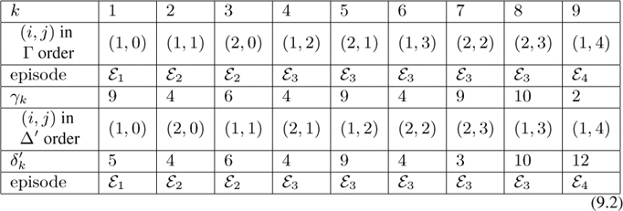
The meaning of the last assertion of Proposition 9.1 is that each indexing visits the episodes of the sequence in order from left to right, and after it is finished with an episode, it moves on to the next with no skipping around. Thus both indexings must be in the same episode.

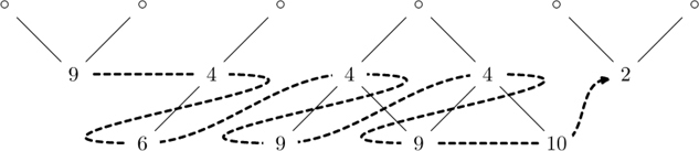
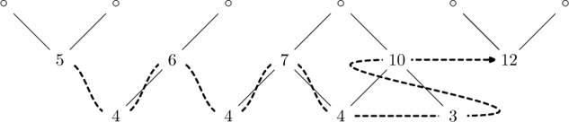
The reason that Proposition 9.1 was called the “Snake Lemma” in [15] is that if one connects the nodes of Θ_B in the indicated orderings, a pair of “snakes” becomes visible. Thus in the example (9.2) the paths will look as follows. The Γ indexing is represented:

and the Δ′ indexing:

• The proof will provide a particular description of the pair of snakes; in applying Proposition 9.1 will sometimes need this particular description. We will describe the pair of indexings, or “snakes,” as canonical if they are produced by the method described in the proof, which is expressed in Table 9.1. Thus we implicitly use the proof as well as the statement of the Lemma.
• If there are resonances, there will be more than one possible pair of snakes. (Indeed, the reader will find another way of drawing the snakes in the preceding example.) These will be obtained through a process of specialization that will be described in the proof. Any one of these pairs of snakes will be described as canonical.

Proof. For this proof, double bonds are irrelevant, and we will work with the bond-unmarked cartoon. Thus both Γ and Δ′ are again represented by the same cartoon, which in the example (8.1) was the cartoon (8.2). Resonances are a minor complication, which we eliminate as follows. We divide the cartoon into panels, each being of one five types:

The first panel of the cartoon is always of type t and the last one of type b. We call a cartoon simple if it contains no panels of type R.

The panel type R occurs at each resonance. Including it in our discussion would unnecessarily increase the number of cases to be considered, so we resolve each resonance by arbitrarily replacing each R by either a T or B. This will produce a simple cartoon. We refer to this process as specialization.

For example the cartoon (8.2) corresponds to the word tBBRTb, meaning that these panels appear in sequence from left to right. We replace the resonant panel R arbitrarily by either T or B; for example if we choose B we obtain the simple cartoon:

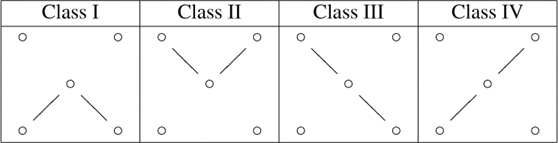
From the simple cartoon we may describe the algorithm for finding the pair of snakes, that is, the Γ and Δ′ indexings. Each connected component (episode) in the simple cartoon has three vertices, the middle one being in the second row. We may classify these episodes into four classes as follows:

Now we can describe the snakes. For each episode, we select a path from Table 9.1. The nodes labeled will turn out to be indexed by even integers, and the nodes labeled • will be indexed by odd integers. We’ve subscripted the ’s to indicate which entries are corresponding in the Γ and Δ′. A ? means that the information at hand does not determine whether the entry will be even or odd in the indexing, so we do not attempt to assign it a or •.

There are modifications at the left and right edges of the pattern: for example, if the first two panels are tB then the first connected component is of Class II, and the left parts of the Γ and Δ′ indexings indicated in the table are missing. Thus we have a modification of the Class II pattern that we call II_t.

Similarly, there are Classes III_t, II_b, and IV_b that can occur at the left or right edge of the pattern. In every case these are obtained by simply deleting part of the corresponding pattern, and we will not enumerate these for this reason.

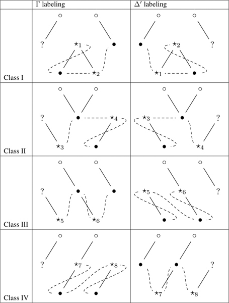
Table 9.1 Snake taxonomy.

It is necessary to see that these paths are assigned consistently. For example, suppose that the cartoon contains consecutive panels TBT. Inside the resulting configuration are both a Class II connected component and a Class I component. Referring to Table 9.1, both these configurations mandate the following dashed line in the Γ diagram.

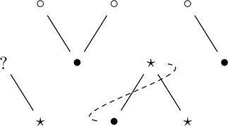
This sort of consistency must be checked in eight cases, which we leave to the reader. Then it is clear that splicing together the segments prescribed this way gives a consistent pair of snakes, and the indexings can be read off from left to right.

It remains, however, for us to prove (9.1). This is accomplished by four Lemmas. There are many things to verify; we will do one and leave the rest to the reader.

LEMMA 9.2 If the j-th connected component is of Class I, then

This asserts a part of (9.1), namely the equality = γ_k for the vertices labeled ₁ and ₂ in Table 9.1, and the equality = γ_k + γ_k−1 − γ_k+1 for the unstarred vertex in the connected component.

We prove that Δ′(1, j) = Γ(2, j). With defined by (6.5) and (6.6) we have

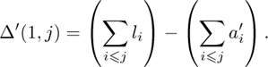
Our assumption that the j-th connected component is of Class I means that l_j ≥ b_j−1 and that l_j+1 ≥ b_j, so = b_j−1 + b_j − a_j. Moreover, since l_j ≥ b_j−1 we have

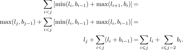
By (6.5) we therefore have

We leave the remaining two statements to the reader.

LEMMA 9.3 If the j-th connected component is of Class II, then

Δ′(1, j) = Γ(1, j) + Γ(2, j − 1) − Γ(1, j + 1).

LEMMA 9.4 If the j-th connected component is of Class III, then

Δ′(1, j) = Γ(2, j),
Δ′(2,j) = Γ(1, j) + Γ(2, j − 1) − Γ(2, j).

LEMMA 9.5 If the j-th connected component is of Class IV, then

Δ′(2, j − 1) = Γ(1, j),

Δ′(1, j) = Γ(2, j − 1) + Γ(1, j) − Γ(1, j + 1).

We leave the proofs of the last three Lemmas to the reader. The assertions in (9.1) are contained in the Lemmas, for each whose corresponding vertex is in the given connected component. It must lie in the first (middle) or second row of the cartoon, which is why there are three identities for Class I, one for Class II, and two for Classes III and IV. Thus (9.1) is proved for every . The final assertion, that the episodes of the cartoon are visited from left to right in order by both indexings, can be seen by inspection from Table 9.1.

LEMMA 9.6 (Circling Lemma) Assume that is strict.

(i) Suppose that either of the following two configurations occurs in either Γ or Δ:

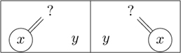
Then x = y.

(ii) If x occurs circled in either the Γ or Δ preaccordions of a strict pattern , then either the same value x also occurs uncircled (and unboxed) at another location, or x = 0.

Proof. The first statement follows from the definition. To prove the second statement, we note that y = x is unboxed since the pattern is strict. If it is uncircled, (ii) is proved. If it is circled, we continue to the right (if y is to the right of x) or to the left (if y is to the left of x) until we come to an uncircled one. This can only fail if we come to the edge of the pattern. If this happens, then x = 0.