
C H A P T E R 3
![]()
SQL for SQLite
This chapter is an introduction to using SQL with SQLite. SQL makes up a huge component of any discussion about databases, and SQLite is no different. Whether you're a novice or pro with SQL, this chapter offers comprehensive coverage. Even if you've never used SQL before, you should have no trouble with the material covered in this chapter. If you've also avoided the relational model that underpins SQLite and other RDBMSs, don't fret. We'll augment our discussion of SQL with just enough of the relational concepts to make things clear, without getting bogged down in the theory.
SQL is the sole (and almost universal) means by which to communicate with a relational database. It is the workhorse devoted to information processing. It is designed for structuring, reading, writing, sorting, filtering, protecting, calculating, generating, grouping, aggregating, and in general managing information.
SQL is an intuitive, user-friendly language. It can be fun to use and is quite powerful. One of the fun things about SQL is that regardless of whether you are an expert or a novice, it seems that you can always continue to learn new ways of doing things (for better or worse).
The goal of this chapter is to teach you to use SQL well—to expose you to good techniques and perhaps a few cheap tricks along the way. As you can already tell from the table of contents, SQL for SQLite is such a large topic that we've split its discussion into two halves. We cover the core select statement first and then move on to other SQL statements in Chapter 4. But by the time you are done, you should be well equipped to put a dent in any database.
![]() Note Even with two chapters, we really only have space to focus on SQL's use in SQLite. For a much wider and in-depth coverage of SQL in general, we recommend a book like Beginning SQL Queries by Claire Churcher.
Note Even with two chapters, we really only have space to focus on SQL's use in SQLite. For a much wider and in-depth coverage of SQL in general, we recommend a book like Beginning SQL Queries by Claire Churcher.
The Example Database
Before diving into syntax, let's get situated with the obligatory example database. The database used in this chapter (and the rest of this book, for that matter) consists of all the foods in every episode of Seinfeld. If you've ever watched Seinfeld, you can't help but notice a slight preoccupation with food. There are more than 400 different foods mentioned in the 180 episodes of its history (according to fan data spread far and wide on the Internet). That's more than two new foods every show. Subtract commercial time, and that's virtually a new food introduced every 10 minutes.
As it turns out, this preoccupation with food works out nicely because it makes for a database that illustrates all the requisite concepts of SQL and of using SQL in SQLite. Figure 3-1 shows the database tables for our sample database.
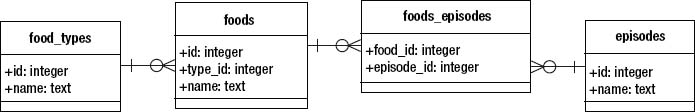
Figure 3-1. The Seinfeld food database
The database schema, as defined in SQLite, is defined as follows:
create table episodes (

  id integer primary key,

  season int,

  name text );


create table foods(

  id integer primary key,

  type_id integer,

  name text );


create table food_types(

  id integer primary key,

  name text );


create table foods_episodes(

  food_id integer,

  episode_id integer );
The main table is foods. Each row in foods corresponds to a distinct food item, the name of which is stored in the name attribute. The type_id attribute references the food_types table, which stores the various food classifications (e.g., baked goods, drinks, or junk food). Finally, the foods_episodes table links foods in foods with the episodes in episodes.
Installation
The food database is located in the examples zip file accompanying this book. It is available on the Apress website (www.apress.com) in the Source Code section. To create the database, first locate the foods.sql file in the root directory of the unpacked zip file. To create a new database from scratch from the command line, navigate to the examples directory, and run the following command:
sqlite3 foods.db < foods.sql
This will create a database file called foods.db. If you are not familiar with how to use the SQLite command-line program, refer to Chapter 2.
Running the Examples
For your convenience, all the SQL examples in the chapter are available in the file sql.sql in the root directory of the examples zip file. So instead of typing them by hand, simply open the file and locate the SQL you want to try.
A convenient way to run the longer queries in this chapter is to copy them into your favorite editor and save them in a separate file, which you can run from the command line. For example, copy a long query in test.sql to try. You simply use the same method to run it as you did to create your database earlier:
sqlite3 foods.db < test.sql
The results will be printed to the screen. This also makes it easier to experiment with these queries without having to retype them or edit them from inside the SQLite shell. You just make your changes in the editor, save the file, and rerun the command line.
For maximum readability of the output, you may want to put the following commands at the beginning of the file:
.echo on

.mode column

.headers on

.nullvalue NULL
This causes the command-line program to 1) echo the SQL as it is executed, 2) print results in column mode, 3) include the column headers, and 4) print nulls as NULL. The output of all examples in this chapter is formatted with these specific settings. Another option you may want to set for various examples is the .width option, which sets the respective column widths of the output. These vary from example to example.
For better readability, the examples are presented in two different formats. For short queries, we'll show the SQL and output as it would be shown from within the SQLite shell. For example:
sqlite> select *

   ...> from foods

   ...> where name='JujyFruit'

   ...> and type_id=9;


id          type_id     name

----------  ----------  ----------

244         9           JujyFruit
Occasionally, as in the previous example, we take the liberty of adding an extra line between the command and its output to improve readability here on the printed page. For longer queries, we show just the SQL in code format separated from the results by gray lines, as in the following example:
select f.name name, types.name type

from foods f

inner join (

  select *

  from food_types

  where id=6) types

on f.type_id=types.id;
name                       type

-------------------------  -----

Generic (as a meal)        Dip

Good Dip                   Dip

Guacamole Dip              Dip

Hummus                     Dip
Syntax
SQL's declarative syntax reads a lot like a natural language. Statements are expressed in the imperative mood, beginning with the verb describing the action. Following it are the subject and predicate, as illustrated in Figure 3-2.
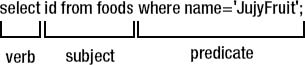
Figure 3-2. General SQL syntax structure
As you can see, it reads like a normal sentence. SQL was designed specifically with nontechnical people in mind and was thus meant to be very simple and easy to understand.
Part of SQL's ease of use comes from its being (for the most part) a declarative language, as opposed to an imperative language such as C or Perl. A declarative language is one in which you describe what you want, whereas an imperative language is one in which you specify how to get it. For example, consider the process of ordering a cheeseburger. As a customer, you use a declarative language to articulate your order. That is, you simply declare to the person behind the counter what you want:
Give me a double meat Whataburger with jalapeños and cheese, hold the mayo.
The order is passed back to the chef who fulfills the order using a program written in an imperative language—the recipe. He follows a series of well-defined steps that must be executed in a specific order to create the cheeseburger per your (declarative) specifications:
- Get ground beef from the third refrigerator on the left.
- Make a patty.
- Cook for three minutes.
- Flip.
- Cook three more minutes.
- Repeat steps 1–5 for second patty.
- Add mustard to top bun.
- Add patties to bottom bun.
- Add cheese, lettuce, tomatoes, onions, and jalapeños to burger.
- Combine top and bottom buns, and wrap in yellow paper.
As you can see, declarative languages tend to be more succinct than imperative ones. In this example, it took the declarative burger language (DBL) one step to materialize the cheeseburger, while it took the imperative chef language (ICL) 10 steps. Declarative languages do more with less. In fact, SQL's ease of use is not far from this example. A suitable SQL equivalent to our imaginary DBL statement shown earlier might be something along the lines of this:
select burger

from kitchen

where patties=2

and toppings='jalopenos'

and condiment != 'mayo'

limit 1;
Pretty simple. As we've mentioned, SQL was designed to be a user-friendly language. In the early days, SQL was targeted specifically for end users for tasks such as ad hoc queries and report generation (unlike today where it is almost exclusively the domain of developers and database administrators).
Commands
SQL is made up of commands. Commands are typically terminated by a semicolon, which marks the end of the command. For example, the following are three distinct commands:
select id, name from foods;

insert into foods values (null, 'Whataburger'),

delete from foods where id=413;
![]() Note The semicolon is used by SQLite as a command terminator, signaling the end of the command to be processed. Command terminators are most commonly associated with interactive programs designed for letting users execute queries against a database. The semicolon is a common SQL command terminator across many systems, though some use
Note The semicolon is used by SQLite as a command terminator, signaling the end of the command to be processed. Command terminators are most commonly associated with interactive programs designed for letting users execute queries against a database. The semicolon is a common SQL command terminator across many systems, though some use g or even the word go.
Commands, in turn, are composed of a series of tokens. Tokens can be literals, keywords, identifiers, expressions, or special characters. Tokens are separated by white space, such as spaces, tabs, and newlines.
Literals
Literals, also called constants, denote explicit values. There are three kinds: string literals, numeric literals, and binary literals. String literals are one or more alphanumeric characters surrounded by single quotes. Here are some examples:
'Jerry'

'Newman'

'JujyFruit'
Although SQLite supports delimiting string values with single or double quotes, we strongly suggest you only use single quotes. This is the SQL standard and will save you many hours of grief should you encounter a system that strictly enforces this. If single quotes are part of the string value, they must be represented as two successive single quotes. For example, Kenny's chicken would be expressed as follows:
'Kenny''s chicken'
Numeric literals are represented in integer, decimal, or scientific notation. Here are some examples:
-1

3.142

6.0221415E23
Binary values are represented using the notation x'0000', where each digit is a hexadecimal value. Binary values must be expressed in multiples of 2 hexadecimal values (8 bits). Here are some examples:
x'01'

X'0fff'

x'0F0EFF'

X'0f0effab'
Keywords and Identifiers
Keywords are words that have a specific meaning in SQL. These include words such as select, update, insert, create, drop, and begin. Identifiers refer to specific objects within the database, such as tables or indexes. Keywords are reserved words and may not be used as identifiers. SQL is case insensitive with respect to keywords and identifiers. The following are equivalent statements:
SELECT * from foo;

SeLeCt * FrOm FOO;
By default, string literal values are case sensitive in SQLite, so the value 'Mike' is not the same as the value 'mike'.
Comments
Comments in SQLite are denoted by two consecutive hyphens (--), which comment the remaining line, or by the multiline C-style notation (/* */), which can span multiple lines. Here's an example:
-- This is a comment on one line

/* This is a comment spanning

   two lines */
Again, unless you have a strong reason to use C-style notation, we'd recommend sticking with the SQL standard of two consecutive hyphens in your SQL scripts for SQLite.
Creating a Database
Tables are the natural starting point to kick off your exploration of SQL in SQLite. The table is the standard unit of information in a relational database. Everything revolves around tables. Tables are composed of rows and columns. And although that sounds simple, tables bring along with them all kinds of other concepts, which can't be nicely summarized in a few tidy paragraphs. In fact, it takes almost the whole chapter. So, what we are going to do here is the two-minute overview of tables—just enough for you to create a simple table and get rid of it if you want to. And once we have that out of the way, all the other parts of this chapter will have something to build on.
Creating Tables
Like the relational model, SQL consists of several parts. It has a structural part, for example, which is designed to create and destroy database objects. This part of the language is generally referred to as a data definition language (DDL). Similarly, it has a functional part for performing operations on those objects (such as retrieving and manipulating data). This part of the language is referred to as a data manipulation language (DML). Creating tables falls under DDL, the structural part.
You create a table with the create table command, which is defined as follows:
create [temp] table table_name (column_definitions [, constraints]);
The temp or temporary keyword creates a temporary table. This kind of table is, well, temporary—it will last only as long your session. As soon as you disconnect, it will be destroyed (if you haven't already destroyed it manually). The brackets around the temp denote that it is an optional part of the command. Whenever you see any syntax in brackets, it means that the contents within them are optional. Furthermore, the pipe symbol (|) denotes an alternative (think of the word or). Take, for example, the following syntax:
create [temp|temporary] table . . . ;
This means that either the temp or temporary keyword may be optionally used. You could say create temp table foo. . ., or you could say create temporary table foo. . .. In this case, they mean the same thing.
If you don't create a temporary table, then create table creates a base table. The term base table refers to a table that is a named, persistent table in the database. This is the most common kind of table. In general, the term base table is used to differentiate tables created by create table from system tables and other table-like objects such as views.
The minimum required information for create table is a table name and a column name. The name of the table, given by table_name, must be unique among all other identifiers. In the body, column_definitions consists of a comma-separated list of column definitions composed of a name, a domain, and a comma-separated list of column constraints. A type, sometimes referred to as a domain, is synonymous with a data type in a programming language. It denotes the type of information that is stored in the column.
There are five native types in SQLite: integer, real, text, blob, and null. All of these types are covered in the section called “Storage Classes” later in this chapter. Constraints are constructs that control what kind of values can be placed in the table or in individual columns. For instance, you can ensure that only unique values are placed in a column by using a unique constraint. Constraints are covered in the section “Data Integrity.”
The create table command allows you to include a list of additional column constraints at the end of the command, denoted by constraints in the syntax outlined earlier. Consider the following example:
create table contacts ( id integer primary key,

                        name text not null collate nocase,

                        phone text not null default 'UNKNOWN',

                        unique (name,phone) );
Column id is declared to have type integer and constraint primary key. As it turns out, the combination of this type and constraint has a special meaning in SQLite. Integer primary key basically turns the column into an autoincrement column (as explained in the section “Primary Key Constraints” later in this chapter). Column name is declared to be of type text and has two constraints: not null and collate nocase. Column phone is of type text and has two constraints defined as well. After that, there is a table-level constraint of unique, which is defined for columns name and phone together.
This is a lot of information to absorb all at once, but it will all be explained in due course. You can probably appreciate our preamble that warned you how complex tables could become. The only important thing here, however, is that you understand the general format of the create table statement.
Altering Tables
You can change parts of a table with the alter table command. SQLite's version of alter table can either rename a table or add columns. The general form of the command is as follows:
alter table table { rename to name | add column column_def }
Note that there is some new notation here: {}. Braces enclose a list of options, where one option is required. In this case, we have to use either alter table table rename. . . or alter table table add column. . .. That is, you can either rename the table using the rename clause or add a column with the add column clause. To rename a table, you simply provide the new name given by name.
If you add a column, the column definition, denoted by column_def, follows the form in the create table statement. It is a name, followed by an optional domain and list of constraints. Here's an example:
sqlite> alter table contacts

        add column email text not null default '' collate nocase;

sqlite> .schema contacts


create table contacts ( id integer primary key,

                        name text not null collate nocase,

                        phone text not null default 'UNKNOWN',

                        email text not null default '' collate nocase,

                        unique (name,phone) );
To view the table definition from within the SQLite command-line program, use the .schema shell command followed by the table name. It will print the current table definition. If you don't provide a table name, then .schema will print the entire database schema.
Tables can also be created from the results of select statements, allowing you to create not only the structure but also the data at the same time. This particular use of the create table statement is covered later in the section “Inserting Records.”
Querying the Database
The effort spent designing your database and creating your tables all focuses on one purpose: using your data. Working with your data is the job of SQL's DML. The core of DML is the select command, which has the unique honor of being the sole command for querying the database. select is by far the largest and most complex command in SQL. select derives many of its operations from relational algebra and encompasses a large portion of it. The capabilities and complexities of the select statement are vast, even in a streamlined efficient environment like SQLite. Don't let that put you off. SQLite's approach to the select command is very logical, and it has a firm grounding in the underlying relational theory that underpins all RDBMS.
Relational Operations
For the theoretically minded, it's useful to think about what select does and why it does it, framed in a conceptual way. In most SQL implementations, including SQLite's, the select statement provides for the “relational operations” that source, mix, compare, and filter data. These relational operations are typically divided into three categories:
- Fundamental operations
- Additional operations
- Intersection
- Natural join
- Assign
- Extended operations
- Generalized projection
- Left outer join
- Right outer join
- Full outer join
The fundamental operations are just that: fundamental. They define the basic relational operations, and all of them (with the exception of rename) have their basis in set theory. The additional operations are for convenience, offering a shorthand way of performing frequently used combinations of the fundamental operations. For instance, intersection can be performed by taking the union of two sets and from that removing via difference the results of two further unions that have each had difference applied for one of the two initial sets. Finally, the extended operations add features to the fundamental and additional operations. For example, the generalized projection operation adds arithmetic expressions, aggregates, and grouping features to the fundamental projection operations. The outer joins extend the join operations and allow additional information and/or incomplete information to be retrieved from the database.
In standard ANSI SQL, select can perform every one of these relational operations. These operations map to the original relational operators defined by E. F. Codd in his original work on relational theory (with the exception of divide). SQLite supports all the relational operations in ANSI SQL with the exception of right and full outer joins. The types of joins can be constructed using combinations of other fundamental relational operations, so don't fret their absence.
All of these operations are defined in terms of relations or, as they are commonly called, tables! They take one or more relations as their inputs and produce a relation as their output. This allows operations to be strung together into relational expressions. Relational expressions can therefore be created to arbitrary complexity. For example, the output of a select operation (a relation) can be fed as the input to another select statement, as follows:
select name from (select name, type_id from (select * from foods));
Here, the output of the innermost select is fed to the next select, whose output is in turn fed to the outermost select. It is all a single relational expression. Anyone familiar with piping commands in Linux, Unix, or Windows will appreciate this behavior. The output of any select statement can be used as input to yet another statement.
select and the Operational Pipeline
The select command incorporates many of the relational operations through a series of clauses in its syntax. Each clause corresponds to specific relational operation. In SQLite, almost all of the clauses are optional, in fact, to a degree beyond what standard SQL suggests is desirable. As a user of SQL in SQLite, this empowers you to employ only the operations you need to obtain the data you seek.
A very general form of select in SQLite (without too much distracting syntax) can be represented as follows:
select [distinct] heading

from tables

where predicate

group by columns

having predicate

order by columns

limit count,offset;
Each keyword—from, where, having, and so on—is a separate clause. Each clause consists of the keyword followed by arguments (represented in italics). From here on out, we will refer to these clauses simply by name, and you'll be able to recognize our use by the fixed-width font. So, rather than “the where clause,” we will simply use where.
In SQLite, the best way to think of the select command is as a pipeline that processes relations. This pipeline has optional processes that you can plug into it as you need them. Regardless of whether you include or exclude a particular operation, the relative operations are always the same. Figure 3-3 shows this order.
The select command starts with from, which takes one or more input relations; combines them into a single composite relation; and passes it through the subsequent chain of operations.
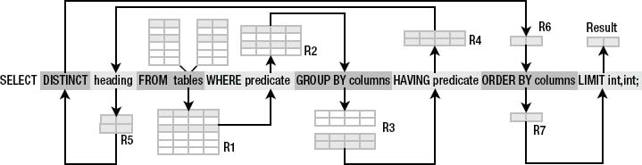
Figure 3-3. The phases of select in SQLite
All clauses are optional with the exception of select. You must always provide at least this clause to make a valid select command. By far the most common invocation of the select command consists of three clauses: select, from, and where. This basic syntax and its associated clauses are as follows:
select heading from tables where predicate;
The from clause is a comma-separated list of one or more tables, views, and so on (represented by the variable tables in Figure 3-3). If more than one table is specified, they will be combined to form a single relation (represented by R1 in Figure 3-3). This is done by one of the join operations. The resulting relation produced by from serves as the initial material. All subsequent operations will either work directly from it or work from derivatives of it.
The where clause filters rows in R1. The argument of where is a predicate, or logical expression, which defines the selection criteria by which rows in R1 are included in (or excluded from) the result. The selected rows from the where clause form a new relation R2, as shown in Figure 3-3 above.
In this particular example, R2 passes through the other operations unscathed until it reaches the select clause. The select clause filters the columns in R2, as depicted in Figure 3-4. Its argument consists of a comma-separated list of columns or expressions that define the result. This is called the projection list, or heading of the result.
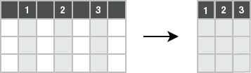
Figure 3-4. Projection
Here's a concrete example using our example database:
sqlite> select id, name from food_types;

id          name

----------  ----------

1           Bakery

2           Cereal

3           Chicken/Fowl

4           Condiments

5           Dairy

6           Dip

7           Drinks

8           Fruit

9           Junkfood

10          Meat

11          Rice/Pasta

12          Sandwiches

13          Seafood

14          Soup

15          Vegetables
There is no where clause to filter rows, so all rows in the table food_types are returned. The select clause specifies all the columns in food_types, and the from clause does not join tables. The result is an exact copy of food_types. As in most SQL implementations, SQLite supports an asterisk (*) as shorthand to mean all columns. Thus, the previous example can just as easily be expressed as follows:
select * from food_types;
In summary, SQLite's basic select processing gathers all data to be considered in the from clause, filters rows (restricts) in the where clause, and filters columns (projects) in the select clause. Figure 3-5 shows this process.
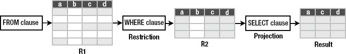
Figure 3-5. Restriction and projection in select
With this simple example, you can begin to see how a query language in general and SQL in particular ultimately operate in terms of relational operations. There is real math under the hood.
Filtering
If the select command is the most complex command in SQL, then the where clause is the most complex clause in select. But it also does most of the work. Having a solid understanding of its mechanics will most likely bring the best overall returns in your day-to-day use of SQL in SQLite.
SQLite applies the where clause to each row of the relation produced by the from clause (R1). As stated earlier, where—a restriction—is a filter. The argument of where is a logical predicate. A predicate, in the simplest sense, is just an assertion about something. Consider the following statement:
The dog (subject) is purple and has a toothy grin (predicate).
The dog is the subject, and the predicate consists of the two assertions (color is purple and grin is toothy). This statement may be true or false, depending on the dog.
The subject in the where clause is a row. The row is the logical subject. The WHERE clause is the logical predicate. Each row in which the proposition evaluates to true is included (or selected) as part of the result (R2). Each row in which it is false is excluded. So, the dog proposition translated into a relational equivalent would look something like this:
select * from dogs where color='purple' and grin='toothy';
The database will take each row in table dogs (the subject) and apply the where clause (the predicate) to form the logical proposition:
This row has color='purple' and grin='toothy'.
If it is true, then the row (or dog) is indeed purple and toothy, and it is included in the result. where is a powerful filter. It provides you with a great degree of control over the conditions with which to include (or exclude) rows in (or from) the result.
Values
Values represent some kind of data in the real world. Values can be classified by their type, such as a numerical value (1, 2, 3, and so on) or string value (“JujyFruit”). Values can be expressed as literal values (an explicit quantity such as 1, 2, 3 or “JujyFruit”), variables (often in the form of column names like foods.name), expressions (3+2/5), or the results of functions (count(foods.name))—which are covered later.
Operators
An operator takes one or more values as input and produces a value as output. An operator is so named because it performs some kind of operation, producing some kind of result. Binary operators are operators that take two input values (or operands). Ternary operators take three operands, unary operators take just one, and so on.
Operators can be strung together, feeding the output of one operator into the input of another (Figure 3-6), forming value expressions.
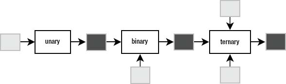
Figure 3-6. Unary, binary, and ternary operators, also displaying pipelining of operations
By stringing operators together, you can create value expressions that are expressed in terms of yet other value expressions to arbitrary complexity. Here's an example:
x = count(episodes.name)

y = count(foods.name)

z = y/x * 11
Binary Operators
Binary operators are by far the most common of all operators in SQL. Table 3-1 lists the binary operators supported in SQLite by precedence, from highest to lowest. Operators in each color group have equal precedence.
Arithmetic operators (for example, addition, subtraction, division) are binary operators that take numeric values and produce a numeric value. Relational operators (for example, >, <, =) are binary operators that compare values and value expressions and return a logical value (also called a truth value), which is either true or false. Relational operators form logical expressions, for example:
x > 5

1 < 2
A logical expression is any expression that returns a truth value. In SQLite, false is represented by the number 0, while true is represented by anything else. For example:
sqlite> SELECT 1 > 2;


1 > 2

----------

0


sqlite> SELECT 1 < 2;


1 < 2

----------

1


sqlite> SELECT 1 = 2;


1 = 2

----------

0


sqlite> SELECT -1 AND 1;


-1 AND 1

----------

1
Logical Operators
Logical operators (AND, OR, NOT, IN) are binary operators that operate on truth values or logical expressions. They produce a specific truth value depending on their inputs. They are used to build more complex logical expressions from simpler expressions, such as the following:
(x > 5) AND (x != 3)

(y < 2) OR (y > 4) AND NOT (y = 0)

(color='purple') AND (grin='toothy')
The truth value produced by a logical operator follows normal Boolean logic rules, but there is an added twist when considering nulls, which we'll discuss later in the chapter. This is the stuff the where clause is made of—using logical operators to answer real questions about the data in your SQLite database. Here's an example:
sqlite> select * from foods where name='JujyFruit' and type_id=9;


id          type_id     name

----------  ----------  ----------

244         9           JujyFruit
The restriction here works according to the expression (name='JujyFruit') and (type_id=9), which consists of two logical expressions joined by logical and. Both of these conditions must be true for any record in foods to be included in the result.
The LIKE and GLOB Operators
A particularly useful relational operator is like. like is similar to equals (=) but is used for matching string values against patterns. For example, to select all rows in foods whose names begin with the letter J, you could do the following:
sqlite> select id, name from foods where name like 'J%';


id     name

-----  --------------------

156    Juice box

236    Juicy Fruit Gum

243    Jello with Bananas

244    JujyFruit

245    Junior Mints

370    Jambalaya
A percent symbol (%) in the pattern matches any sequence of zero or more characters in the string. An underscore (_) in the pattern matches any single character in the string. The percent symbol is greedy. It will eat everything between two characters except those characters. If it is on the extreme left or right of a pattern, it will consume everything on each respective side. Consider the following examples:
sqlite> select id, name from foods where name like '%ac%P%';


id     name

-----  --------------------

127    Guacamole Dip

168    Peach Schnapps

198    Mackinaw Peaches
Another useful trick is to use NOT to negate a pattern:
sqlite> select id, name from foods

        where name like '%ac%P%' and name not like '%Sch%'


id     name

-----  --------------------

 38     Pie (Blackberry) Pie

127    Guacamole Dip

198    Mackinaw peaches
The glob operator is very similar in behavior to the like operator. Its key difference is that it behaves much like Unix or Linux file globbing semantics in those operating systems. This means it uses the wildcards associated with file globbing such as * and _ and that matching is case sensitive. The following example demonstrates glob in action:
sqlite> select id, name from foods

   ...> where name glob 'Pine*';


id          name

----------  ----------

205         Pineapple

258         Pineapple
SQLite also recognizes the match and regexp predicates but currently does not provide a native implementation. You'll need to develop your own with the sqlite_create_funtion() call, discussed in Chapters 5 through 8.
Limiting and Ordering
You can limit the size and particular range of the result using the limit and offset keywords. limit specifies the maximum number of records to return. offset specifies the number of records to skip. For example, the following statement obtains the Cereal record (the second record in food_types) using limit and offset:
select * from food_types order by id limit 1 offset 1;
The offset clause skips one row (the Bakery row), and the limit clause returns a maximum of one row (the Cereal row).
But there is something else here as well: order by. This clause sorts the result by a column or columns before it is returned. The reason it is important in this example is because the rows returned from select are never guaranteed to be in any specific order—the SQL standard declares this. Thus, the order by clause is essential if you need to count on the result being in any specific order. The syntax of the order by clause is similar to the select clause: it is a comma-separated list of columns. Each entry may be qualified with a sort order—asc (ascending, the default) or desc (descending). For example:
sqlite> select * from foods where name like 'B%'

        order by type_id desc, name limit 10;


id     type_id   name

-----  --------  --------------------

382    15        Baked Beans

383    15        Baked Potato w/Sour

384    15        Big Salad

385    15        Broccoli

362    14        Bouillabaisse

328    12        BLT

327    12        Bacon Club (no turke

326    12        Bologna

329    12        Brisket Sandwich

274    10        Bacon
Typically you only need to order by a second (third, and so on) column when there are duplicate values in the first (second, and so on) ordered column(s). Here, there were many duplicate type_ids. I wanted to group them together and then arrange the foods alphabetically within these groups.
![]() Note
Note limit and offset are not standard SQL keywords as defined in the ANSI standard. Most databases have functional equivalents, although they use different syntax.
If you use both limit and offset together, you can use a comma notation in place of the offset keyword. For example, the following SQL:
select * from foods where name like 'B%'

order by type_id desc, name limit 1 offset 2;
can be expressed equivalently with this:
sqlite> select * from foods where name like 'B%'

        order by type_id desc, name limit 2,1;


id     type_id   name

-----  --------  --------------------

384    15        Big Salad
There is a trick here for those who think this syntax should be the other way around. In SQLite, when using this shorthand notation, the offset precedes the limit. Here, the values following limit keyword specify an offset of 2 and a limit of 2. Also, note that offset depends on limit. That is, you can use limit without using offset but not the other way around.
Notice that limit and offset are dead last in the operational pipeline. One common misconception of limit/offset is that it speeds up a query by limiting the number of rows that must be collected by the where clause. This is not true. If it were, then order by would not work properly. For order by to do its job, it must have the entire result in hand to provide the correct order. There is a small performance boost, in that SQLite only needs to keep track of the order of the 10 biggest values at any point. This has some benefit but not nearly as much as the “sort-free limiting” that some expect.
Functions and Aggregates
SQLite comes with various built-in functions and aggregates that can be used within various clauses. Function types range from mathematical functions such as abs(), which computes the absolute value, to string-formatting functions such as upper() and lower(), which convert text to upper- and lowercase, respectively. For example:
sqlite> select upper('hello newman'), length('hello newman'), abs(-12);


upper('hello newman')  length('hello newman') abs(-12)

---------------------  --------------------   ----------

HELLO NEWMAN           12                     12
Notice that the function names are case insensitive (i.e., upper() and UPPER() refer to the same function). Functions can accept column values as their arguments:
sqlite> select id, upper(name), length(name) from foods

        where type_id=1 limit 10;


id     upper(name)                 length(name)

-----  --------------------------  ------------

1      BAGELS                      6

2      BAGELS, RAISIN              14

3      BAVARIAN CREAM PIE          18

4      BEAR CLAWS                  10

5      BLACK AND WHITE COOKIES     23

6      BREAD (WITH NUTS)           17

7      BUTTERFINGERS               13

8      CARROT CAKE                 11

9      CHIPS AHOY COOKIES          18

10     CHOCOLATE BOBKA             15
Since functions can be part of any expression, they can also be used in the where clause:
sqlite> select id, upper(name), length(name) from foods

        where length(name) < 5 limit 5;


id     upper(name)           length(name)

-----  --------------------  --------------------

36     PIE                   3

48     BRAN                  4

56     KIX                   3

57     LIFE                  4

80     DUCK                  4
Aggregates are a special class of functions that calculate a composite (or aggregate) value over a group of rows (or relation). Standard aggregate functions include sum(), avg(), count(), min(), and max(). For example, to get a count of the number of foods that are baked goods (type_id=1), you can use the count aggregate as follows:
sqlite> select count(*) from foods where type_id=1;


count

-----

47
The count aggregate returns a count of every row in the relation. Whenever you see an aggregate, you should automatically think, “For each row in a table, do something.”
Aggregates can aggregate not only column values but any expression—including functions. For example, to get the average length of all food names, you can apply the avg aggregate to the length(name) expression as follows:
sqlite> select avg(length(name)) from foods;


avg(length(name))

-----------------

12.58
Aggregates operate within the select clause. They compute their values on the rows selected by the where clause—not from all rows selected by the from clause. The select command filters first and then aggregates.
Although SQLite comes with a standard set of common SQL functions and aggregates, it is worth noting that the SQLite C API allows you to create custom functions and aggregates as well. See Chapter 7 for more information.
Grouping
An essential part of aggregation is grouping. That is, in addition to computing aggregates over an entire result, you can also split that result into groups of rows with like values and compute aggregates on each group—all in one step. This is the job of the group by clause. Here's an example:
sqlite> select type_id from foods group by type_id;


type_id

----------

1

2

3

.

.

.

15
group by is a bit different from the other parts of select, so you need to use your imagination a little to wrap your head around it. Figure 3-7 illustrates the process. Operationally, group by sits in between the where clause and the select clause. group by takes the output of where and splits it into groups of rows that share a common value (or values) for a specific column (or columns). These groups are then passed to the select clause. In the example, there are 15 different food types (type_id ranges from 1 to 15), and therefore group by organizes all rows in foods into 15 groups varying by type_id. select takes each group, extracts its common type_id value, and puts it into a separate row. Thus, there are 15 rows in the result, one for each group.
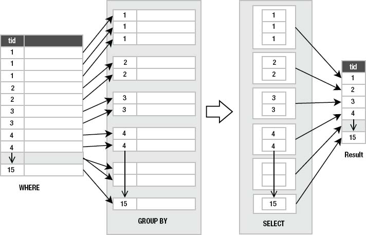
Figure 3-7. group by process
When group by is used, the select clause applies aggregates to each group separately, rather than the entire result as a whole. Since aggregates produce a single value from a group of values, they collapse these groups of rows into single rows. For example, consider applying the count aggregate to the preceding example to get the number of records in each type_id group:
sqlite> select type_id, count(*) from foods group by type_id;


type_id     count(*)

----------  ----------

1           47

2           15

3           23
4           22

5           17

6           4

7           60

8           23

9           61

10          36

11          16

12          23

13          14

14          19

15          32
Here, count() was applied 15 times—once for each group, as illustrated in Figure 3-8. Note that in the diagram, the actual number of records in each group is not represented literally (that is, it doesn't show 47 records in the group for type_id=1).
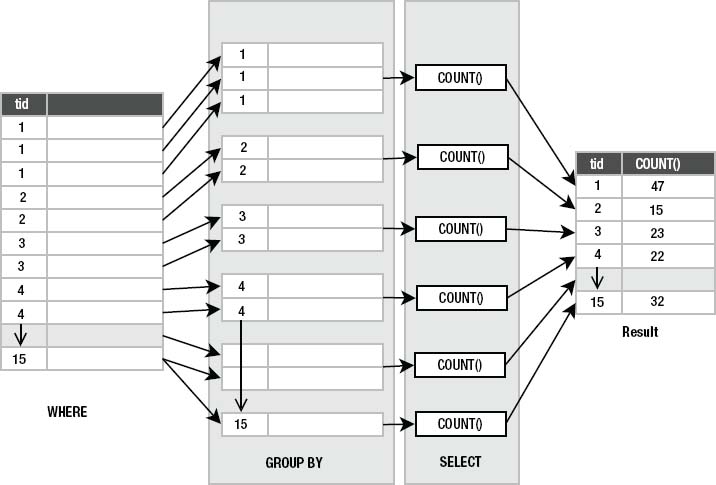
Figure 3-8. group by and aggregation
The number of records with type_id=1 (Baked Goods) is 47. The number with type_id=2 (Cereal) is 15. The number with type_id=3 (Chicken/Fowl) is 23, and so forth. So, to get this information, you could run 15 queries as follows:
select count(*) from foods where type_id=1;

select count(*) from foods where type_id=2;

select count(*) from foods where type_id=3;

.

.

.

select count(*) from foods where type_id=15;
Or, you get the results using the single select with a group by as follows:
select type_id, count(*) from foods group by type_id;
But there is more. Since group by has to do all this work to create groups with like values, it seems a pity not to let you filter these groups before handing them off to the select clause. That is the purpose of having, a predicate that you apply to the result of group by. It filters the groups from group by in the same way that the where clause filters rows from the from clause. The only difference is that the where clause's predicate is expressed in terms of individual row values, and having's predicate is expressed in terms of aggregate values.
Take the previous example, but this time say you are interested only in looking at the food groups that have fewer than 20 foods in them:
sqlite> select type_id, count(*) from foods

        group by type_id having count(*) < 20;


type_id     count(*)

----------  ----------

2           15

5           17

6           4

11          16

13          14

14          19
Here, having applies the predicate count(*)<20 to all the groups. Any group that does not satisfy this condition (that has 20 or more foods in it) is not passed on to the select clause. Figure 3-9 illustrates this restriction.
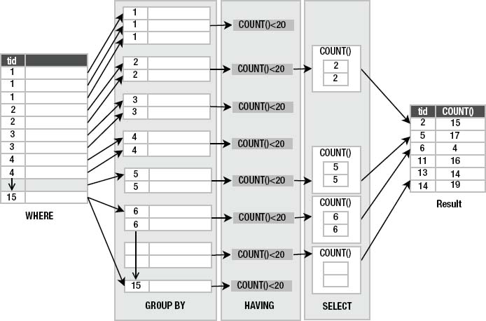
Figure 3-9. having as group restriction
The third column in the figure shows groups of rows ordered by type_id. The values shown are the type_id values. The actual number of rows shown in each group is not exact but figurative. I have only shown two rows in each group to represent the group as a whole.
So, group by and having work as additional restriction phases. group by takes the restriction produced by the where clause and breaks it into groups of rows that share a common value for a given column. having then applies a filter to each of these groups. The groups that make it through are passed on to the select clause for aggregation and projection.
![]() Caution Some databases, including SQLite, will allow you to construct a
Caution Some databases, including SQLite, will allow you to construct a select statement where nonaggregated columns are not grouped in a select statement with mixed aggregate and nonaggregate columns. For instance, SQLite will allow you to execute this SQL:
select type_id, count(*) from foods
Because the aggregate (count) collapses the input table, there is a mismatch in the number of rows that pass all the filtering steps. Count in this case will return one row, but we haven't instructed SQLite how to group type_id. Nevertheless, SQLite will return something. Sadly, the results of such a statement are meaningless—do not rely on any SQL statement that doesn't group by nonaggregate fields. The results are arbitrary!
Removing Duplicates
distinct takes the result of the select clause and filters out duplicate rows. For example, you'd use this to get all distinct type_id values from foods:
sqlite> select distinct type_id from foods;


type_id

----------

1

2

3

.

.

.

15
This statement works as follows: the where clause returns the entire foods table (all 412 records). The select clause pulls out just the type_id column, and finally distinct removes duplicate rows, reducing the number from 412 rows to 15 rows, all unique.
Joining Tables
Joins are the key to working with data from multiple tables (or relations) and are the first operation(s) of the select command. The result of a join is provided as the input or starting point for all subsequent (filtering) operations in the select command.
Joins in SQLite are best understood by example. The foods table has a column type_id. As it turns out, the values in this column correspond to values in the id column in the food_types table. A relationship exists between the two tables. Any value in the foods.type_id column must correspond to a value in the food_types.id column, and the id column is the primary key (described later) of food_types. The foods.type_id column, by virtue of this relationship, is called a foreign key: it contains (or references) values in the primary key of another table. This relationship is called a foreign key relationship
Using this relationship, it is possible to join the foods and food_type tables on these two columns to make a new relation, which provides more detailed information, namely, the food_types.name for each food in the foods table. This is done with the following SQL:
sqlite> select foods.name, food_types.name

        from foods, food_types

        where foods.type_id=food_types.id limit 10;


name                       name

-------------------------  ---------------

Bagels                     Bakery

Bagels, raisin             Bakery

Bavarian Cream Pie         Bakery

Bear Claws                 Bakery

Black and White cookies    Bakery

Bread (with nuts)          Bakery

Butterfingers              Bakery

Carrot Cake                Bakery

Chips Ahoy Cookies         Bakery

Chocolate Bobka            Bakery
You can see the foods.name in the first column of the result, followed by the food_types.name in the second. Each row in the former is linked to its associated row in the latter using the foods.type_id → food_types.id relationship (Figure 3-10).
![]() Note We are using a new notation in this example to specify the columns in the
Note We are using a new notation in this example to specify the columns in the select clause. Rather than specifying just the column names, we are using the notation table_name.column_name. The reason is that we have multiple tables in the select statement. The database is smart enough to figure out which table a column belongs to—as long as that column name is unique among all tables. If you use a column whose name is also defined in other tables of the join, the database will not be able to figure out which of the columns you are referring to and will return an error. In practice, when you are joining tables, it is always a good idea to use the table_name.column_name notation to avoid any possible ambiguity. This is explained in detail in the section “Names and Aliases.”
To carry out the join, the database finds these matched rows. For each row in the first table, the database finds all rows in the second table that have the same value for the joined columns and includes them in the input relation. So in this example, the from clause built a composite relation by joining the rows of two tables.
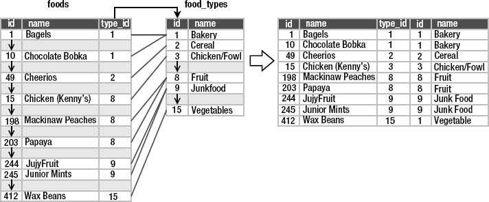
Figure 3-10. foods and food_types join
The subsequent operations (where, group by, and so on) work exactly the same. It is only the input that has changed through joining tables. As it turns out, SQLite supports six different kinds of joins. The one just described, called an inner join, is the most common.
Inner Joins
An inner join is where two tables are joined by a relationship between two columns in the tables, as in this previous example. It is the most common (and perhaps most generally useful) type of join.
An inner join uses another set operation in relational algebra, called an intersection, to find elements that exist in both sets. Figure 3-11 illustrates this. The intersection of the set {1, 2, 8, 9} and the set {1, 3, 5, 8} is the set {1, 8}. The intersection operation is represented by a Venn diagram showing the common elements of both sets.
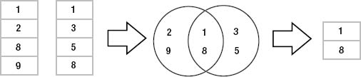
This is precisely how an inner join works, but the sets in a join are common elements of the related columns. Pretend that the left set in Figure 3-11 represents values in the foods.type_id column and the right set represents values of the food_types.id column. Given the matching columns, an inner join finds the rows from both sides that contain like values and combines them to form the rows of the result (Figure 3-12). Note that this example assumes that the records shown are the only records in foods and food_types.
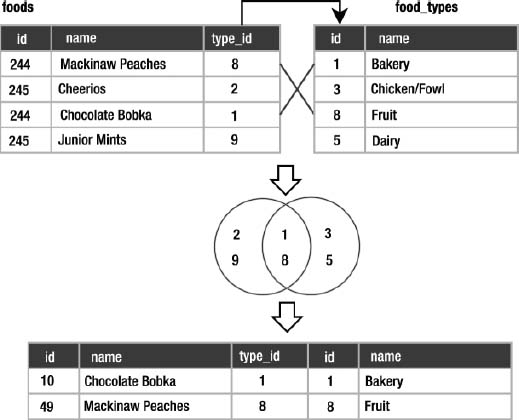
Figure 3-12. Food join as intersection
Inner joins only return rows that satisfy the given column relationship, also called the join condition. They answer the question, “What rows of B match rows in A given the following relationship?” Let's demonstrate this in SQL so you can match the theory with a practical example.
Select *

From foods inner join food_types on foods.id = food_types.id
The syntax is clearly understandable once you've visualized what's happening.
Cross Joins
Imagine for a moment that there is no join condition. What would you get? In this case, if the two tables were not related in any way, select would produce a more fundamental kind of join (the mostfundamental), which is called a cross join, Cartesian join, or cross product. The Cartesian join is one of the fundamental relational operations. It is a brute-force, almost nonsensical join that results in the combination of all rows from the first table with all rows in the second.
In SQL, the cross join of foods and food_types is expressed as follows:
select * from foods, food_types;
from, in the absence of anything else, produces a cross join. The result is shown here. Every row in foods is combined with every row in food_types, but crucially, not by relating the id and type_id values. In a cross join, no relationship exists between the rows; there is no join condition, but they are simply jammed together.
1           1           Bagels      1           Bakery

1           1           Bagels      2           Cereal

1           1           Bagels      3           Chicken/Fowl

. . .

(6174 rows omitted to save paper)

. . .

412         15          Wax Beans   13          Seafood

412         15          Wax Beans   14          Soup

412         15          Wax Beans   15          Vegetables
You may ask yourself what purpose such a cross join has. To be frank, that's the question you should always ask yourself before using such logic. Do you really want the cross-product of every row in one table with every row in another. The answer is almost always no.
Outer Joins
Three of the remaining four joins are called outer joins. An inner join selects rows across tables according to a given relationship. An outer join selects all the rows of an inner join plus some rows outside of the relationship. The three outer join types are called left, right, and full. A left outer join operates with respect to the “left table” in the SQL command. For example, in the command:
select *

from foods left outer join foods_episodes on foods.id=foods_episodes.food_id;
foods is the left table here. The left outer join favors it. It is the table of significance in a left outer join. The left outer join tries to match every row of foods with every row in foods_episodes per the join condition (foods.id=foods_episodes.food_id). All such matching rows are included in the result. However, if we had registered some foodstuffs in the foods table that had not yet appeared in an episode, the remaining food rows of foods that don't match foods_episodes are still included in the result, and where foods_episodes hasn't provide a row, it “supplies” null results.
The right outer join works similarly, except the right table is the one whose rows are included, matching or not. Operationally, left and right outer joins are identical; they do the same thing. They differ only in order and syntax. As a user of SQLite, that means any problem that can requires a right outer join for solution can equally be solved with a left outer join.
A full outer join is the combination of a left and right outer join. It includes all matching records, followed by unmatched records in the right and left tables. Currently, both right and full outer joins are not supported in SQLite. However, as mentioned earlier, a right join can be replaced with a left outer join, and a full outer join can be performed using compound queries (see the section “Compound Queries” later in this chapter).
Natural Joins
The last join on the list is called a natural join. It is actually an inner join in disguise, but with a little syntax and convention thrown in. A natural join joins two tables by their common column names. Thus, using the natural join, you can get the inner join of two tables without having to add the join condition.
Natural joins will join all columns by the same name in both tables. Just the process of adding to or removing a column from a table can drastically change the results of a natural join query. This can produce very unpredictable results, especially if your tables' design change over time. It's always better to explicitly define the join conditions of your queries than rely on the semantics of the table schema.
Preferred Syntax
Syntactically, there are various ways of specifying a join. The inner join example of foods and food_types illustrates performing a join implicitly in the where clause:
select * from foods, food_types where foods.id=food_types.food_id;
When the database sees more than one table listed, it knows there will be a join—at the very least a cross join. The where clause here calls for an inner join.
This implicit form, although rather clean, is actually an older form of syntax that you should avoid. The politically correct way (per SQL92) to express a join in SQL is using the join keyword. The general form is as follows:
select heading from left_table join_type right_table on join_condition;
This explicit form can be used for all join types. For example:
select * from foods inner join food_types on foods.id=food_types.food_id;

select * from foods left outer join food_types on foods.id=food_types.food_id;

select * from foods cross join food_types;
The most important reason for using ANSI join syntax is that there are some query types that can only be satisfied by using the join keyword-style syntax. This is particularly so for any form of outer join—left, right, or full.
Names and Aliases
When joining tables, ambiguity can arise if both tables have a column with the same name. If you were to join two tables with and id column using a select id clause in the earlier code, which id should SQLite return? To help with this type of task, you can qualify column names with their table names to remove any ambiguity, as you saw earlier.
Another useful feature is aliases. If your table name is particularly long and you don't want to have to use its name every time you qualify a column, you can use an alias. Aliasing is actually a fundamental relational operation called rename. The rename operation simply assigns a new name to a relation. For example, consider this statement:
select foods.name, food_types.name

from foods, food_types

where foods.type_id = food_types.id

limit 10;
There is a good bit of typing here. You can alias the tables in the source clause by simply including the new name directly after the table name, as in the following example:
select f.name, t.name

from foods f, food_types t

where f.type_id = t.id

limit 10;
Here, the foods table is assigned the alias f, and the food_types table is assigned the alias t. Now, every other reference to foods or food_types in the statement must use the alias f and t, respectively. Aliases make it possible to do self-joins—joining a table with itself. For example, say you want to know what foods in season 4 are mentioned in other seasons. You would first need to get a list of episodes and foods in season 4, which you would obtain by joining episodes and episodes_foods. But then you would need a similar list for foods outside of season 4. Finally, you would combine the two lists based on their common foods. The following query uses self-joins to do the trick:
select f.name as food, e1.name, e1.season, e2.name, e2.season

from episodes e1, foods_episodes fe1, foods f,

     episodes e2, foods_episodes fe2

where

  -- Get foods in season 4

  (e1.id = fe1.episode_id and e1.season = 4) and fe1.food_id = f.id

  -- Link foods with all other episodes

  and (fe1.food_id = fe2.food_id)

  -- Link with their respective episodes and filter out e1's season

  and (fe2.episode_id = e2.id AND e2.season != e1.season)

order by f.name;


food                  name               season  name                     season

--------------------  -----------------  ------  -----------------------  ------

Bouillabaisse         The Shoes          4       The Stake Out            1

Decaf Cappuccino      The Pitch          4       The Good Samaritan       3

Decaf Cappuccino      The Ticket         4       The Good Samaritan       3

Egg Salad             The Trip 1         4       Male Unbonding           1

Egg Salad             The Trip 1         4       The Stock Tip            1

Mints                 The Trip 1         4       The Cartoon              9

Snapple               The Virgin         4       The Abstinence           8

Tic Tacs              The Trip 1         4       The Merv Griffin Show    9

Tic Tacs              The Contest        4       The Merv Griffin Show    9

Tuna                  The Trip 1         4       The Stall                5

Turkey Club           The Bubble Boy     4       The Soup                 6

Turkey Club           The Bubble Boy     4       The Wizard               9
I have put comments in the SQL to better explain what is going on. This example uses two self-joins using the where clause join syntax. There are two instances of episodes and foods_episodes, but they are treated as if they are two independent tables. The query joins foods_episodes back on itself to link the two instances of episodes. The two episodes instances are related to each other by an inequality condition to ensure that they are in different seasons. You can alias column names and expressions in the same way. The general alias syntax in SQLite is the same in all cases.
Select base-name [[as] alias] . . .
The as keyword is optional, but many people prefer it because it makes the aliasing more legible, and it makes you less likely to confuse an alias with a base column name or expression.
Subqueries
Subqueries are select statements within select statements. They are also called subselects. Subqueries are useful in many ways, they work anywhere normal expressions work, and they can therefore be used in a variety of places in a select statement. Subqueries are useful in other commands as well.
Perhaps the most common use of subqueries is in the where clause, specifically using the in operator. The in operator is a binary operator that takes an input value and a list of values and returns true if the input value exists in the list, or false otherwise. Here's an example:
sqlite> select 1 in (1,2,3);

1

sqlite> select 2 in (3,4,5);

0

sqlite> select count(*)

   ...> from foods

   ...> where type_id in (1,2);

62
Using a subquery, you can rewrite the last statement in terms of names from the food_types:
sqlite> select count(*)

   ...> from foods

   ...> where type_id in

   ...>  (select id

   ...>   from food_types

   ...>   where name='Bakery' or name='Cereal'),

62
Subqueries in the select clause can be used to add additional data from other tables to the result set. For example, to get the number of episodes each food appears in, the actual count from foods_episodes can be performed in a subquery in the select clause:
sqlite> select name,

        (select count(id) from foods_episodes where food_id=f.id) count

        from foods f order by count desc limit 10;


name            count

----------      ----------

Hot Dog         5

Pizza           4

Ketchup         4
Kasha           4

Shrimp          3

Lobster         3

Turkey Sandwich 3

Turkey Club     3

Egg Salad       3

Tic Tacs        3
The order by and limit clauses here serve to create a top ten list, with hot dogs at the top. Notice that the subquery's predicate references a table in the enclosing select command: food_id=f.id. The variable f.id exists in the outer query. The subquery in this example is called a correlated subquery because it references, or correlates to, a variable in the outer (enclosing) query.
Subqueries can be used in the order by clause as well. The following SQL groups foods by the size of their respective food groups, from greatest to least:
select * from foods f

order by (select count(type_id)

from foods where type_id=f.type_id) desc;
order by in this case does not refer to any specific column in the result. How does this work then? The order by subquery is run for each row, and the result is associated with the given row. You can think of it as an invisible column in the result set, which is used to order rows.
Finally, we have the from clause. There may be times when you want to join to the results of another query, rather than to a base table. It's yet another job for a subquery:
select f.name, types.name from foods f

inner join (select * from food_types where id=6) types

on f.type_id=types.id;
name                       name

-------------------------  -----

Generic (as a meal)        Dip

Good Dip                   Dip

Guacamole Dip              Dip

Hummus                     Dip
Notice that the use of a subquery in the from clause requires a rename operation. In this case, the subquery was named types. Subqueries as a source relation in the from clause are often called inline views or derived tables.
The thing to remember about subqueries is that they can be used anywhere a relational expression can be used. A good way to learn how, where, and when to use them is to just play around with them and see what you can get away with. There is often more than one way to skin a cat in SQL. When you understand the big picture, you can make more informed decisions on when a query might be rewritten to run more efficiently.
Compound Queries
Compound queries are kind of the inverse of subqueries. A compound query is a query that processes the results of multiple queries using three specific relational operations: union, intersection, and difference. In SQLite, these are defined using the union, intersect, and except keywords, respectively.
Compound query operations require a few things of their arguments:
- The relations involved must have the same number of columns.
- There can be only one
order byclause, which is at the end of the compound query and applies to the combined result.
Furthermore, relations in compound queries are processed from left to right.
The union operation takes two relations, A and B, and combines them into a single relation containing all distinct rows of A and B. In SQL, union combines the results of two select statements. By default, union eliminates duplicates. If you want duplicates included in the result, then use union all. For example, the following SQL finds the single most and single least frequently mentioned foods:
select f.*, top_foods.count from foods f

inner join

  (select food_id, count(food_id) as count from foods_episodes

     group by food_id

     order by count(food_id) desc limit 1) top_foods

  on f.id=top_foods.food_id

union

select f.*, bottom_foods.count from foods f

inner join

  (select food_id, count(food_id) as count from foods_episodes

     group by food_id

     order by count(food_id) limit 1) bottom_foods

  on f.id=bottom_foods.food_id

order by top_foods.count desc;
id     type_id  name       top_foods.count

-----  -------  ---------  ---------------

288    10       Hot Dog    5

1      1        Bagels     1
Both queries return only one row. The only difference in the two is which way they sort their results. The union simply combines the two rows into a single relation.
The intersect operation takes two relations, A and B, and selects all rows in A that also exist in B. The following SQL uses intersect to find the all-time top ten foods that appear in seasons 3 through 5:
select f.* from foods f

inner join

  (select food_id, count(food_id) as count

     from foods_episodes

     group by food_id

     order by count(food_id) desc limit 10) top_foods

  on f.id=top_foods.food_id
intersect

select f.* from foods f

  inner join foods_episodes fe on f.id = fe.food_id

  inner join episodes e on fe.episode_id = e.id

  where e.season between 3 and 5

order by f.name;
id     type_id  name

-----  -------  --------------------

4      1        Bear Claws

146    7        Decaf Cappuccino

153    7        Hennigen's

55     2        Kasha

94     4        Ketchup

164    7        Naya Water

317    11       Pizza
To produce the top ten foods, we needed an order by in the first select statement. Since compound queries allow only one order by at the end of the statement, we got around this by performing an inner join on a subquery in which we computed the top ten most common foods. Subqueries can have order by clauses because they run independently of the compound query. The inner join then produces a relation containing the top ten foods. The second query returns a relation containing all foods in episodes 3 through 5. The intersect operation then finds all matching rows.
The except operation takes two relations, A and B, and finds all rows in A that are not in B. By changing the intersect to except in the previous example, you can find which top ten foods are not in seasons 3 through 5:
select f.* from foods f

inner join

  (select food_id, count(food_id) as count from foods_episodes

     group by food_id

     order by count(food_id) desc limit 10) top_foods

  on f.id=top_foods.food_id

except

select f.* from foods f

  inner join foods_episodes fe on f.id = fe.food_id

  inner join episodes e on fe.episode_id = e.id

  where e.season between 3 and 5

order by f.name;
id     type_id  name

-----  -------  --------

192    8        Banana

133    7        Bosco

288    10       Hot Dog
As mentioned earlier, what is called the except operation in SQL is referred to as the difference operation in relational algebra.
Compound queries are useful when you need to process similar data sets that are materialized in different ways. Basically, if you cannot express everything you want in a single select statement, you can use a compound query to get part of what you want in one select statement and part in another (and perhaps more) and process the sets accordingly.
Conditional Results
The case expression allows you to handle various conditions within a select statement. There are two forms. The first and simplest form takes a static value and lists various case values linked to return values:
case value

  when x then value_x

  when y then value_y

  when z then value_z

  else default_value

end
Here's a simple example:
select name || case type_id

                 when 7  then ' is a drink'

                 when 8  then ' is a fruit'

                 when 9  then ' is junkfood'

                 when 13 then ' is seafood'

                 else null

               end description

from foods

where description is not null

order by name

limit 10;
description

---------------------------------------------

All Day Sucker is junkfood

Almond Joy is junkfood

Apple is a fruit

Apple Cider is a drink

Apple Pie is a fruit

Arabian Mocha Java (beans) is a drink

Avocado is a fruit

Banana is a fruit

Beaujolais is a drink

Beer is a drink
The case expression in this example handles a few different type_id values, returning a string appropriate for each one. The returned value is called description, as qualified after the end keyword. This string is concatenated to name by the string concatenation operator (||), making a complete sentence. For all type_ids not specified in a when condition, case returns null. The select statement filters out such null values in the where clause, so all that is returned are rows that the case expression does handle.
The second form of case allows for expressions in the when condition. It has the following form:
case

  when condition1 then value1

  when condition2 then value2

  when condition3 then value3

  else default_value

end
CASE works equally well in subselects comparing aggregates. The following SQL picks out frequently mentioned foods:
select name,(select

               case

                 when count(*) > 4 then 'Very High'

                 when count(*) = 4 then 'High'

                 when count(*) in (2,3) then 'Moderate'

                 else 'Low'

               end

             from foods_episodes

             where food_id=f.id) frequency

from foods f

where frequency like '%High'
name       frequency

---------  ----------

Kasha      High

Ketchup    High

Hot Dog    Very High

Pizza      High
This query runs a subquery for each row in foods that classifies the food by the number of episodes it appears in. The result of this subquery is included as a column called frequency. The where predicate filters frequency values that have the word High in them.
Only one condition is executed in a case expression. If more than one condition is satisfied, only the first of them is executed. If no conditions are satisfied and no else condition is defined, case returns null.
Handling Null in SQLite
Most relational databases support the concept of “unknown” or “unknowable” through a special placeholder called null, which is a placeholder for missing information and is not a value per se. Rather, null is the absence of a value: null is not nothing, null is not something, null is not true, null is not false, null is not zero, null is not an empty string. Simply put, null is resolutely what it is: null. And not everyone can agree on what that means. There are a few key rules and ideas that you should learn so you can master the use of null in SQLite.
First, in order to accommodate null in logical expressions, SQL uses something called three-value (or tristate) logic, where null is one of the truth values. Table 3-2 shows the truth table for logical and and logical or with null thrown into the mix.
Table 3-2. AND and OR with NULL
| x | y | x AND y | y OR y |
| True True | True | True | |
| True False | False | True | |
| True | NULL NULL |
True | |
| False False | False | False | |
| False | NULL |
False | NULL |
NULL NULL |
NULL |
NULL |
You can try a few simple select statements to see the effect of null yourself.
Second, detecting the presence or absence of null is done using the is null or is not null operator. If you try to use any other operator, such as equals, greater than, and so on, you will receive a shock, which leads us to our third rule regarding null.
Third and last, always remember that null is not equal to any other value, even null itself. You cannot compare null with a value, and no null is greater than, smaller than, or in any way related to any another null. This often catches out the unwary when statements like the next example fail to return any rows.
select *

from mytable

where myvalue = null;
Nothing can equal null, so no data will ever be returned by that statement in SQLite. Now that you've mastered the basics, you'll be pleased to know that SQLite offers several additional functions for working with null. The first of which is a workaround for the very limitation of “nothing equals NULL” that we've just drilled in to you. From SQLite v 3.6.19, the is operator can be used to equate one NULL to another. In the most basic form, you can run a simple query to ask SQLite if NULL is NULL:
sqlite> select NULL is NULL;

1
As already mentioned, any value other than zero means “true,” so SQLite is happy to tell us that in this instance NULL really is the same as NULL. But please, don't rely on this heavily. SQL's trivalue logic may be awkward, but it is a standard, and working around it with the is operator will likely have you encountering problems with other systems and programming languages that expect the standard behavior.
The coalesce function, which is part of the SQL99 standard, takes a list of values and returns the first non-null in the list. Take the following example:
select coalesce(null, 7, null, 4)
In this case, coalesce will return 7 as the first non-null value. This is also handy when performing arithmetic, so you can detect whether null has been returned and return a meaningful value like 0 instead.
Conversely, the nullif function takes two arguments and returns null if they have the same values; otherwise, it returns the first argument:
sqlite> select nullif(1,1);

null

sqlite> select nullif(1,2);

1
If you use null, you need to take special care in queries that refer to columns that may contain null in their predicates and aggregates. null can do quite a number on aggregates if you are not careful.
Summary
Congratulations, you have learned the select command for SQLite's implementation of SQL. Not only have you learned how the command works, but you've learned some relational theory in the process. You should now be comfortable with using select statements to query your data, join, aggregate, summarize, and dissect it for various uses.
We'll continue the discussion of SQL in the next chapter, where we'll build on your knowledge of select by introducing the other members of DML, as well as DDL and other helpful SQL constructs in SQLite.