
Chapter 4. Variables
A variable stores a value in memory so that it can be used later in a program. The variable can be used many times within a single program, and the value is easily changed while the program is running.
First Variables
One of the reasons we use variables is to avoid repeating ourselves in the code. If you are typing the same number more than once, consider making it into a variable to make your code more general and easier to update.
Example 4-1: Reuse the Same Values
For instance, when you make the y coordinate and diameter for the two circles in this example into variables, the same values are used for each ellipse:

size(480,120)y=60d=80ellipse(75,y,d,d)# Leftellipse(175,y,d,d)# Middleellipse(275,y,d,d)# Right
Example 4-2: Change Values
Simply changing the y and d variables alters all three ellipses:

size(480,120)y=100d=130ellipse(75,y,d,d)# Leftellipse(175,y,d,d)# Middleellipse(275,y,d,d)# Right
Without the variables, you’d need to change the y coordinate used in the code three times and the diameter six times. When comparing Example 4-1 and Example 4-2, notice how the bottom three lines of code are the same, and only the middle two lines with the variables are different. Variables allow you to separate the lines of the code that change from the lines that don’t, which makes programs easier to modify. For instance, if you place variables that control colors and sizes of shapes in one place, then you can quickly explore different visual options by focusing on only a few lines of code.
Making Variables
When you make your own variables, you determine the name and the value. The name is what you decide to call the variable. Choose a name that is informative about what the variable stores, but be consistent and not too verbose. For instance, the variable name “radius” will be clearer than “r” when you look at the code later.
The range of values that can be stored within a variable is defined by its data type. For instance, the integer data type can store numbers without decimal places (whole numbers). There are data types to store each kind of data: integers, floating-point (decimal) numbers, words, images, fonts, and so on. Python automatically determines the data type of a variable based on the value you assign to it.
Processing Variables
Processing has a series of special variables to store information about the program while it runs. For instance, the width and height of the window are stored in variables called width and height. These values are set by the size() function. They can be used to draw elements relative to the size of the window, even if the size() line changes.
Example 4-3: Adjust the Size, See What Follows
In this example, change the parameters to size() to see how it works:

size(480,120)line(0,0,width,height)# Line from (0,0) to (480, 120)line(width,0,0,height)# Line from (480, 0) to (0, 120)ellipse(width/2,height/2,60,60)
Other special variables keep track of the status of the mouse and keyboard values and much more. These are discussed in Chapter 5.
A Little Math
People often assume that math and programming are the same thing. Although knowledge of math can be useful for certain types of coding, basic arithmetic covers the most important parts.
Example 4-4: Basic Arithmetic

size(480,120)x=25h=20y=25rect(x,y,300,h)# Topx=x+100rect(x,y+h,300,h)# Middlex=x-250rect(x,y+h*2,300,h)# Bottom
In code, symbols like +, -, and * are called operators. When placed between two values, they create an expression. For instance, 5 + 9 and 1024 - 512 are both expressions. The operators for the basic math operations are:
|
+ |
Addition |
|
− |
Subtraction |
|
* |
Multiplication |
|
/ |
Division |
|
= |
Assignment |
Python has a set of rules to define which operators take precedence over others, meaning which calculations are made first, second, third, and so on. These rules define the order in which the code is run. A little knowledge about this goes a long way toward understanding how a short line of code like this works:
x=4+4*5# Assign 24 to x
The expression 4 * 5 is evaluated first because multiplication has the highest priority. Second, 4 is added to the product of 4 * 5 to yield 24. This is clarified with parentheses, but the result is the same:
x=4+(4*5)# Assign 24 to x
If you want to force the addition to happen first, just move the parentheses. Because parentheses have a higher precedence than multiplication, the order is changed and the calculation is affected:
x=(4+4)*5# Assign 40 to x
An acronym for this order is often taught in math class: PEMDAS, which stands for Parentheses, Exponents, Multiplication, Division, Addition, Subtraction, where parentheses have the highest priority and subtraction the lowest. The complete order of operations is found in Appendix C.
Some calculations are used so frequently in programming that shortcuts have been developed; it’s always nice to save a few keystrokes. For instance, you can add to a variable, or subtract from it, with a single operator:
x+=10# This is the same as x = x + 10y−=15# This is the same as y = y - 15
Repetition
As you write more programs, you’ll notice that patterns occur when lines of code are repeated, but with slight variations. A code structure called a for loop makes it possible to run a line of code more than once to condense this type of repetition into fewer lines. This makes your programs more modular and easier to change.
Example 4-5: Do the Same Thing Over and Over
This example has the type of pattern that can be simplified with a for loop:

size(480,120)strokeWeight(8)line(20,40,80,80)line(80,40,140,80)line(140,40,200,80)line(200,40,260,80)line(260,40,320,80)line(320,40,380,80)line(380,40,440,80)
Example 4-6: Use a for Loop
The same thing can be done with a for loop, and with less code:
size(480,120)strokeWeight(8)foriinrange(20,400,60):line(i,40,i+60,80)
The for loop is different in many ways from the code we’ve written so far. Notice the colon (:) at the end of the line that begins with for, and how the line directly beneath it is indented (i.e., moved over from the lefthand margin with some whitespace). The indented code between the braces is called a block. This is the code that will be repeated on each iteration of the for loop.
The for loop has several moving parts. Between the word for and the word in, there is a variable name, which we’ll call the target variable. Inside the parentheses, following the word range, there are three values, separated by commas: start, stop, and step. These three values determine how many times the code inside the block is run, and what value the target variable will have on each iteration of the loop:
fortarget_variableinrange(start,stop,step):statements
The start value determines what value the target variable will have on the first iteration of the loop. On the second iteration of the loop, the step will be added to the start value, and the value of the target_variable will reflect this. This continues until the resulting value is greater than or equal to the step value, at which point the loop terminates.
You can use whatever name you’d like for the target variable, as long as it’s a valid variable name in Python. The variable name i is frequently used, but there’s really nothing special about it.
Example 4-7: Flex Your for Loop’s Muscles
The ultimate power of working with a for loop is the ability to make quick changes to the code. Because the code inside the block is typically run multiple times, a change to the block is magnified when the code is run. By modifying Example 4-6 only slightly, we can create a range of different patterns:

size(480,120)strokeWeight(2)foriinrange(20,400,8):line(i,40,i+60,80)
Example 4-8: Fanning Out the Lines

size(480,120)strokeWeight(2)foriinrange(20,400,20):line(i,0,i+i/2,80)
Example 4-9: Kinking the Lines
In this example, we’re drawing two lines inside of the for loop (not just one). Both statements are indented, which tells Python that both statements should be executed for each iteration of the loop. It’s important in Python to use exactly the same keystrokes to indent multiple statements in the same for loop. (Otherwise, you might get a syntax error.) For example, if the first statement in the for loop is indented with two space characters, the second statement must be indented with two space characters as well.

size(480,120)strokeWeight(2)foriinrange(20,400,20):line(i,0,i+i/2,80)line(i+i/2,80,i*1.2,120)
Example 4-10: Embed One for Loop in Another
When one for loop is embedded inside another, the number of repetitions is multiplied. First, let’s look at a short example, and then we’ll break it down in Example 4-11:

size(480,120)background(0)noStroke()foryinrange(0,height+45,40):forxinrange(0,width+45,40):fill(255,140)ellipse(x,y,40,40)
Example 4-11: Rows and Columns
In this example, the for loops are adjacent, rather than one embedded inside the other. The result shows that one for loop is drawing a column of four circles and the other is drawing a row of 13 circles:

size(480,120)background(0)noStroke()foryinrange(0,height+45,40):fill(255,140)ellipse(0,y,40,40)forxinrange(0,width+45,40):fill(255,140)ellipse(x,0,40,40)
When one of these for loops is placed inside the other, as in Example 4-10, the four repetitions of the first loop are compounded with the 13 of the second in order to run the code inside the embedded block 52 times (4×13 = 52).
Example 4-10 is a good base for exploring many types of repeating visual patterns. The following examples show a couple of ways that it can be extended, but this is only a tiny sample of what’s possible. In Example 4-12, the code draws a line from each point in the grid to the center of the screen. In Example 4-13, the ellipses shrink with each new row and are moved to the right by adding the y coordinate to the x coordinate.
Example 4-12: Pins and Lines
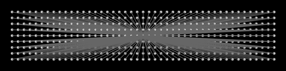
size(480,120)background(0)fill(255)stroke(102)foryinrange(20,height-15,10):forxinrange(20,width-15,10):ellipse(x,y,4,4)# Draw a line to the center of the displayline(x,y,240,60)
Example 4-13: Halftone Dots

size(480,120)background(0)foryinrange(32,height,8):forxinrange(12,width,15):ellipse(x+y,y,16-y/10.0,16-y/10.0)
Robot 2: Variables

The variables introduced in this program make the code look more difficult than Robot 1 (see “Robot 1: Draw”), but now it’s much easier to modify, because numbers that depend on one another are in a single location. For instance, the neck can be drawn based on the bodyHeight variable. The group of variables at the top of the code control the aspects of the robot that we want to change: location, body height, and neck height. You can see some of the range of possible variations in the figure. From left to right, here are the values that correspond to them:
y = 390 bodyHeight = 180 neckHeight = 40 |
y = 460 bodyHeight = 260 neckHeight = 95 |
y = 310 bodyHeight = 80 neckHeight = 10 |
y = 420 bodyHeight = 110 neckHeight = 140 |
When altering your own code to use variables instead of numbers, plan the changes carefully, then make the modifications in short steps. For instance, when this program was written, each variable was created one at a time to minimize the complexity of the transition. After a variable was added and the code was run to ensure it was working, the next variable was added:
x=60# x coordinatey=420# y coordinatebodyHeight=110# Body heightneckHeight=140# Neck heightradius=45# Head radiusny=y-bodyHeight-neckHeight-radius# Neck Ysize(170,480)strokeWeight(2)background(0,153,204)ellipseMode(RADIUS)# Neckstroke(102)line(x+2,y-bodyHeight,x+2,ny)line(x+12,y-bodyHeight,x+12,ny)line(x+22,y-bodyHeight,x+22,ny)# Antennaeline(x+12,ny,x-18,ny-43)line(x+12,ny,x+42,ny-99)line(x+12,ny,x+78,ny+15)# BodynoStroke()fill(255,204,0)ellipse(x,y-33,33,33)fill(0)rect(x-45,y-bodyHeight,90,bodyHeight-33)fill(102)rect(x-45,y-bodyHeight+17,90,6)# Headfill(0)ellipse(x+12,ny,radius,radius)fill(255)ellipse(x+24,ny-6,14,14)fill(0)ellipse(x+24,ny-6,3,3)fill(153)ellipse(x,ny-8,5,5)ellipse(x+30,ny-26,4,4)ellipse(x+41,ny+6,3,3)