2

Maximum Power Point Tracking

2.1    The Dynamic Optimization Problem

Chapter 1 was extensively dedicated to the discussion of the main aspects concerning the current vs. voltage characteristics of a PV generator and its dependency on the exogenous uncontrollable temperature and sun irradiance variables. The in-depth analysis has shown evidence that the joint variation of temperature and irradiance, as well as the occurrence of drift phenomena that arise along the PV system lifetime, about 25 years, makes the position of the maximum power point (MPP) varying in a wide area. As a consequence, a direct connection of the PV generator to the input port of a power processing system imposing a constant voltage level would be a simple but poor choice from the energy productivity point of view. For instance, a PV battery charger obtained by connecting merely the PV array terminals to the battery would force the PV generator to work at a constant voltage. If this voltage is higher than the PV array open-circuit voltage, then the PV system does not deliver any electric power. Otherwise, the closer the battery voltage to the actual V_MPP, the higher the electrical power generated by the PV array. Unfortunately, due to the inherent time variability of V_MPP caused by the changes in the operating conditions, the probability that the PV array delivers the maximum power at any time of the day is almost near zero.

The same conclusion holds if the PV array feeds a resistive load, because the intersection between the resistor characteristic and the I-V curve of the PV array cannot always occur in the MPP for the whole day, so that a power lower than the maximum one is delivered to the load. Figures 2.1 and 2.2 show that the operating point resulting from a straightforward connection of a PV generator with a battery or a resistive load cannot be the MPP in any irradiance or temperature condition.

As a consequence, it is mandatory to adopt an intermediate conversion stage, interfacing the PV array and the power system that processes or uses the electrical power produced thereof, which must be capable of adapting its input voltage and current levels to the instantaneous PV source MPP, while keeping its output voltage and current levels compliant with the load requirement. Such a stage must be a dynamical optimizator, which means that it must be able to perform this adaptation in the presence of time-varying operating conditions affecting the PV generator. The adoption of a linear regulator would be ineffective from the efficiency point of view, so that a switching converter is almost always employed. Because of the reduced cost of power devices, the adoption of a switching converter is now in use from very low power levels, e.g., energy scavenging, up to high power applications, e.g., in large solar power plants. Nevertheless, because the additional electronic device increases the system cost, a trade-off between power maximization and system cost must be reached. Indeed, very high-energy efficiency, above 95%, is required to fully exploit the benefits of power electronics in maximizing the energy productivity of PV plants. A careful selection of power converters architecture and power devices is needed to achieve such results. This point is discussed in depth in Chapter 5.

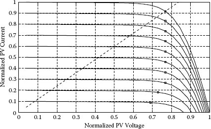
FIGURE 2.1
Operating conditions resulting from a straight connection of a PV generator with a resistive load at varying irradiance levels. Squares are the MPPs.

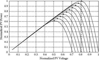
FIGURE 2.2
Operating conditions resulting from a straight connection of a PV generator with a battery at varying temperatures. Squares are the MPPs.

In order to ensure the maximization of the power extracted from the PV source, the interface power converter must be capable of self-adjusting its own parameters at run time, thus changing its input voltage/current levels based on the PV source MPP position. In this book it is assumed, unless specified differently, that the dynamical optimizator is a DC/DC converter and that the control parameter is the duty cycle d of the main switch, as shown in Figure 2.3.

Supposing that the DC/DC voltage conversion ratio of the converter is M(d) = V_o/V_i, the equivalent resistance and voltage seen at the PV source terminals can be expressed by (2.1):

$R_{in}\left(d\right)=\frac{R_{Load}}{M{\left(d\right)}^2};V_i\left(d\right)=\frac{V_0}{M\left(d\right)}$

(2.1)

Figure 2.4 shows the effect of the duty cycle modification in the PV operating point when it is connected to a DC/DC converter and supplies a resistive load (Figure 2.4a) or a constant voltage load like a battery (Figure 2.4b).

The duty cycle value d must be changed continuously by a controller to ensure that the PV generator always operates at its MPP for whatever irradiance and temperature operating conditions: For this reason it is called maximum power point tracking (MPPT) controller. Based on the instantaneous values of the current and voltage sensed at the PV generator terminals, the MPPT controller dynamically adjusts the converter duty cycle to follow the MPP, as shown in Figure 2.5.

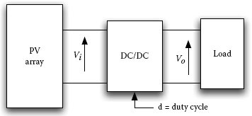
FIGURE 2.3
Connection scheme of a DC/DC converter dedicated to the dynamical optimization of a PV generator.

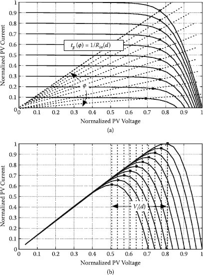
FIGURE 2.4
Operating conditions resulting from a PV generator interfaced to a DC/DC converter. In (a) the PV source has been characterized for different irradiance levels, and in (b) the PV source has been characterized for different temperature levels.

In most applications, the MPPT controller is conceived to maximize the power extracted from the PV generator. Nevertheless, it might be more convenient to employ the MPPT controller for maximizing the power extracted from the switching converter output terminals, thus transferred to the end user. The difference between the maximization of the input power and that of the output power of the switching converter is in the intrinsic variation of the converter efficiency, which is conditioned by the change of the operating point during the day. In fact, it should be considered that the irradiation variations cause a significant change of operating current stress on power devices, whose losses are related, in turn, to physical parameters that are heavily conditioned by the temperature. Moreover, in nonuniform irradiance conditions, additional voltage stress is imposed to power devices, as shown in Chapters 4 and 5. All these factors sum up negatively in causing the efficiency of the converter to lower. As a consequence, an increase in the PV power may determine operating conditions for the converter that lead to a lower efficiency, thus potentially resulting in a lower power at the converter output. In literature, the maximization of the power extracted from the PV source is mostly considered the main problem, because the efficiency vs. power rate profile of the power converter is supposed to be designed so that the higher the PV power, the higher the efficiency. However, this point must be carefully considered when a power converter is designed for PV applications, as the power devices must be selected trying to trade off the cost limitations with the need to guarantee a proper shape of the efficiency vs. the power rate according to the power conversion architecture and to the control strategy adopted for the entire system. For this reason, the PV power maximization problem is considered in this book under the perspective of global energy productivity. Chapter 5 provides a detailed discussion of this point.

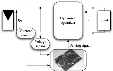
FIGURE 2.5
MPPT implementation.

The MPPT techniques presented in literature and used in most commercial products usually measure both the PV current and voltage values. Direct sensing of the temperature and irradiance is normally avoided, as their measurement requires expensive devices that have to be placed throughout the PV generator, in order to get the values of such variables for each panel or group of them, thus making the measurement quite expensive, especially for large PV plants.

The MPPT controller can be realized based on different methods and algorithms. The most popular methods are known as perturb and observe (P&O) and incremental conductance (INC). The former is widely used in commercial products and is the basis of the largest part of the most sophisticated algorithms presented in literature. Due to the fact that, as explained in the sequel, the INC approach can be seen as an improved version of the P&O one, this chapter devotes most of its space to the P&O approach.

The practical implementation of MPPT controllers is mostly realized in digital form. The speed of analog-to-digital converters needed to realize MPPT based on digital control is not a critical matter because of the relatively slow variation of the temperature and irradiance to be followed. The computations required by MPPT algorithms allow the designer to use cheap microcontrollers, for basic P&O and INC approaches, or much more expensive devices, like digital signal processing (DSP) and field-programmable gate array (FPGA) systems, when the MPPT approach is based on much more involved and burdensome computations, as those required by neural networks and fuzzy logic techniques. A brief overview of the soft computing approaches to the MPPT problem is given in Section 2.3.

The adoption of a digital controller is not strictly necessary for the MPPT implementation. In fact, it is possible to use analog circuitry to realize the MPPT controller as well [1]. Analog control, however, is not much used in PV MPPT applications because of the difficulty encountered in the design of the controller to take into account tolerances and parametric drifts. The flexibility and the possibility to realize self-adaptive controllers offered by the digital implementation justify the very limited adoption of analog control. However, better performances together with the possibility of ease and cheap realization of distributed MPPT applications are prerogatives of analog MPPT controllers. Brief descriptions of the few techniques that can be implemented by means of analog circuitry only are given in Sections 2.2, 2.6.2, and 2.7.1.

In this chapter, the MPPT problem is discussed with reference to a PV array working in uniform irradiance and temperature operating conditions. Specific distributed MPPT architectures and control algorithms needed for applications where PV generators are subjected to shadowing and other mismatching effects, discussed in the first chapter and for which the P-V curve can exhibit more than one maximum power point, are treated in Chapter 4.

2.2    Fractional Open-Circuit Voltage and Short-Circuit Current

In this section, some typical approaches in which the MPP is estimated by using information extracted by the models of the PV generator are discussed. In some cases, they greatly depend on the system behavior in a particular operating condition, in which some electrical variables can be easily measured.

Such methods are usually defined as indirect MPPT techniques because they do not measure the power extracted by the PV source, so that the maximum power point can be only approximately tracked. The main drawback of such techniques is that when the real conditions deviate too much with respect to those supposed in the modeled adopted, e.g., for the effect of parametric drifts, the energy losses are significant.

Alternatively, if the MPPT capability must be assured with high precision and in every environmental condition the PV source is operating in, then direct MPPT methods are more appropriate. In such techniques the PV current and voltage are measured continuously, and such measurements are used to realize a proper adjustment of the system operating conditions in order to catch the MPP.

Indirect MPPT methods are based on the estimation or on occasional measurement of one current or one voltage. In [2] it is shown that the MPP is typically located at a voltage close to 76% of the open-circuit voltage of the PV panel. In a more recent study [3], a more reasonable range of 70–82% has been indicated for the percent ratio between V_MPP and V_OC. A method for tracking the MPP without using an involved algorithm was deduced from this observation based on experimental evaluation on a number of PV panels available on the market. Such a method is quite simple and cheap. A switch connected in series with the PV module is used to disconnect the PV source periodically to allow measurement of its open-circuit voltage and, afterwards, to force the PV system to work at a voltage level that is 76% of the measured voltage. In any case, this method also requires a decoupling unit (e.g., a switching converter) between the source and the load, so that the desired voltage can be settled at the PV source terminals.

This is the weak point of such an approach, which also has a heavy limitation in the fact that the magic number 76% does not hold for any operating condition and for any PV panel. Moreover, it is easy to understand that, during the time interval used for measuring the open-circuit voltage, the PV generator does not feed energy. The higher the irradiation level at which the measure is done, the larger the missed energy.

In [4] it is stated that the I_MPP value is 86% of the short-circuit current; thus the dual approach might be applied by measuring periodically the short-circuit current instead of the open-circuit voltage. The same comments above apply to such a dual approach.

2.3    Soft Computing Methods

Fuzzy and neural network methods can be very useful in affording a hard nonlinear problem, as MPPT is.

Fuzzy logic-based trackers have shown very good performances under varying irradiance conditions without any detailed knowledge of the PV source model. The other side of the coin is that deep knowledge of the system operation and experience are required to choose the relevant computation error and the rule base table. Moreover, neural network strategies require specific training for each type of PV panel or array, and they need new training periods if the long-term parametric drifts are to be accounted for. Such a limitation has been overcome in [5] by using a genetic algorithm to achieve an optimal tuning of the membership functions. Improved performances with respect to the classical MPPT voltage-based approach have also been demonstrated in [6]. The Takagi-Sugeno (T-S) fuzzy approach proposed therein does not require any coordinate transformation, employs simple fuzzy rules, and is able to track rapid irradiance variations.

2.4    The Perturb and Observe Approach

The perturb and observe (P&O) method is the most popular algorithm belonging to the class of the direct MPPT techniques; it is characterized by the injection of a small perturbation into the system, whose effects are used to drive the operating point toward the MPP. Other methods derived by the P&O approach are the incremental conductance (INC), the self-oscillation (SO) method, and the extremum seeking (ES) control. Such methods differ from the P&O approach either for the variable observed or for the type of perturbation. All these algorithms have the advantage of being independent of the knowledge of the PV generator characteristics, so that the MPP is tracked regardless of the irradiance level, temperature, degradation, and aging, thus ensuring high robustness and reliability.

The first use of the P&O technique for tracking the MPP in PV systems goes back to the 1970s, when it was used intensively for aerospace applications [7]. At that time a fully analog implementation was adopted; nowadays, with the progress of the performances of low-cost microcontrollers, the digital implementation is preferred because the implementation of the MPPT algorithm results in a simple code [8].

The P&O method is based on the following concept: The PV operating point is perturbed periodically by changing the voltage at PV source terminals, and after each perturbation, the control algorithm compares the values of the power fed by the PV source before and after the perturbation. If after the perturbation the PV power has increased, this means that the operating point has been moved toward the MPP; consequently, the subsequent perturbation imposed to the voltage will have the same sign as the previous one. If after a voltage perturbation the power drawn from the PV array decreases, this means that the operating point has been moved away from the MPP. Therefore the sign of the subsequent voltage perturbation is reversed. The switching converter is used to drive the perturbation of the operating voltage of the PV generator.

FIGURE 2.6
Basic schemes for implementing the P&O algorithm.

Two basic P&O configurations can be adopted for controlling the switching converter and realizing the PV source voltage perturbation: The first one involves a direct perturbation of the duty ratio of the power converter. In the second one the perturbation is applied to the reference voltage of an error amplifier that generates the signal controlling the duty cycle. Both solutions are shown in Figure 2.6. In the first case, the converter operates in open loop after each duty cycle perturbation, while in the second case the converter is equipped with a feedback voltage loop.

The general equation describing the P&O algorithm is

$x_{\left(\left(k+1\right)T_p\right)}=x_{\left(k{T}_p\right)}\pm \text{Δ}x=x_{\left(k{T}_p\right)}+\left(x_{\left(k{T}_p\right)}-x_{\left(\left(k-1\right)T_p\right)}\right)\cdot sign\left(P_{\left(k{T}_p\right)}-P_{\left(\left(k-1\right)T_p\right)}\right)$

(2.2)

where x represents the variable that is perturbed (e.g., the duty cycle or the feedback voltage reference in the schemes shown in Figure 2.6); T_p is the time interval between two perturbations, in the sequel referred to as perturbation period; Δx is the amplitude of the perturbation imposed to x, in the sequel referred to as perturbation amplitude; and P is the power extracted from the PV array. Figure 2.7 shows the flowchart of the P&O algorithm based on Equation (2.2).

The basic version of the P&O algorithm uses a fixed step amplitude Δx = |x_(kTp) − x_(k−1)Tp| that is selected on the basis of performance trade-off between transient rise time and steady-state conditions.

Figure 2.8 shows the operating points of the PV field imposed step-by-step by the P&O algorithm. When the system approaches the MPP, the perturbing nature of the P&O and other similar MPPT algorithms involves oscillations across the MPP whose characteristics depend on the value of the parameters {Δx, Tp} in (2.2). In [9] it was shown that the minimum number of steps that ensures a periodic and stable oscillation around the MPP is three, corresponding to a 2Δx peak-to-peak amplitude and a periodicity of 4T_p. Such condition is likely the optimal one: Further steps to the left or right side would move the operating point far from the MPP, thus reducing the average power extracted from the PV field. Regardless of the Δx amplitude, a stable three-point behavior is ensured if the time interval T_p is properly selected. If it is settled at a small value, the P&O algorithm can be confused and the operating point can become unstable, entering disordered or chaotic behaviors [10]. On the contrary, a too big value of T_p penalizes the MPPT speed. Guidelines for optimal design of the couple of parameters {Δx, T_p} are given in the following section.

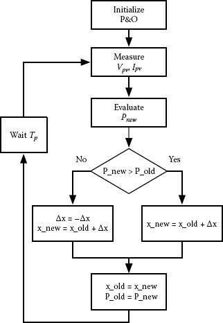
FIGURE 2.7
Basic flowchart for implementing the P&O algorithm.

In literature some variants of the P&O algorithm have been presented. They are especially aimed at reducing the amplitude of the oscillations around the MPP in steady-state irradiance and temperature conditions and at increasing the tracking performances during cloudy days. Although the design guidelines given in the next section refer to the basic P&O algorithm, they can be easily extended to other perturbative approaches.

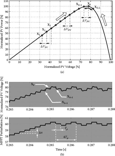
FIGURE 2.8
PV operating points imposed by the P&O algorithm. (a) Power vs. voltage characteristic. (b) Time domain behavior.

2.4.1    Performance Optimization: Steady-State and Dynamic Conditions

Unless sensing input voltage and current of a switching power converter, the MPPT controller works on it as a sampled data feedback system. Due to the nonlinearity of its equation (2.2), it cannot be analyzed/designed by using the classical approaches used for linear regulators, e.g., by analyzing the Bode plots of the loop gain transfer function in the Laplace domain. However, linear open-loop operation between perturbations allows use of time domain analysis. Therefore the design procedure discussed in the following is based on time domain analysis, both in steady-state environmental conditions and in the presence of irradiance variations. Time domain analysis allows optimization of the values of the two P&O parameters {Δx, T_p} separately.

As shown in [10], the results obtained by using the time domain analysis are in agreement with those achievable by means of the describing function method, mostly used for feedback nonlinear system analysis.

By referring to the schemes of Figure 2.6, the intrinsic dynamic nature of the switching converters introduces a propagation delay between the stimulus Δx and the variables measured for estimating the PV power. If the time delay is greater than T_p, the P&O algorithm has no correct information for deciding the sign of the next perturbation. In order to identify the minimum value to assign to T_p, the behavior of the whole system can be analyzed by considering the system small-signal model evaluated around the MPP. Regarding the PV source, if the oscillations of the operating point v_PV, i_PV) are small compared to (V_MPP, I_MPP), then the relationship among i_PV, v_PV, G, and T can be linearized as follows:

${\widehat{i}}_{PV}={\frac{\partial i_{PV}}{\partial v_{PV}}|}_{MPP}\cdot {\widehat{v}}_{PV}+{\frac{\partial i_{PV}}{\partial G}|}_{MPP}\cdot \widehat{G}+{\frac{\partial i_{PV}}{\partial T}|}_{MPP}\cdot \widehat{T}$

(2.3)

where symbols with hats represent small-signal variations around the steady-state values of the corresponding quantities.

At a constant irradiance level it is $\widehat{G}=0$. Moreover, in steady state, due to the relatively high thermal inertia of the PV array [11], the amplitude of variations of the PV array temperature, as a consequence of small oscillations of the operating point, is negligible: Then $\widehat{T}=0$. Therefore (2.3) can be rewritten as

${{\widehat{i}}_{PV}=\frac{\partial i_{PV}}{\partial v_{PV}}|}_{MPP}\cdot {\widehat{v}}_{PV}$

(2.4)

where, based on the models introduced in Chapter 1, the derivative of the PV current with respect to the PV voltage can be expressed as follows:

$\frac{\partial i_{PV}}{\partial v_{PV}}=-{\left[R_s+\frac{1}{\frac{I_{sat}}{\eta \cdot V_t}\cdot e^{\frac{vPV+R_s\cdot iPV}{\eta \cdot V_t}}+\frac{1}{R_p}}\right]}^{-1}$

(2.5)

R_s, R_p, V_t, and I_sat are the values of the parameters of the model of the whole PV field: They have been obtained by scaling the corresponding parameters of a single module for the numbers of modules inside the field (Equations (1.14)–(1.17)).

In any operating point close to the MPP it is

$v_{PV}=V_{MPP}+{\widehat{v}}_{PV}$

(2.6)

$i_{PV}=I_{MPP}+{\widehat{i}}_{PV}$

(2.7)

$p_{PV}=P_{MPP}+{\widehat{p}}_{PV}=V_{MPP}\cdot I_{MPP}+V_{MPP}.{\widehat{i}}_{PV}+I_{MPP\cdot }{\widehat{v}}_{PV}+{\widehat{v}}_{PV}\cdot {\widehat{i}}_{PV}$

(2.8)

Under steady-state conditions in terms of irradiance level and temperature, the MPP occurs where the derivative of the power with respect to the PV voltage is equal to zero:

${\frac{\partial p_{PV}}{\partial v_{PV}}|}_{MPP}=0$

(2.9)

Writing 2.9 as a function of the PV current and voltage yields

${\frac{\partial p_{PV}}{\partial v_{PV}}|}_{MPP}={\frac{\partial \left(v_{PV}\cdot i_{PV}\right)}{\partial v_{PV}}|}_{MPP}={\left(i_{PV}+v_{PV}\cdot \frac{\partial i_{PV}}{\partial v_{PV}}\right)|}_{MPP}=0$

(2.10)

Let us then define the differential resistance R_MPP of the PV array at the MPP:

$\frac{1}{R_{MPP}}={-\frac{\partial i_{PV}}{\partial v_{PV}}|}_{MPP}$

(2.11)

Accordingly, (2.10) can be rewritten as

$\frac{1}{R_{MPP}}={\frac{i_{PV}}{v_{PV}}|}_{MPP}=\frac{I_{MPP}}{V_{MPP}}$

(2.12)

From (2.8), (2.4), and (2.12) it results that

$P_{MPP}=V_{MPP}\cdot I_{MPP}$

(2.13)

${\widehat{p}}_{PV}={\widehat{v}}_{PV}\cdot \left(I_{MPP}-\frac{V_{MPP}}{R_{MPP}}\right)+{\widehat{v}}_{PV}\cdot {\widehat{i}}_{PV}=-\frac{{\widehat{v}}^2{}_{PV}}{R_{MPP}}$

(2.14)

This is a general result that is not dependent on the DC/DC converter topology adopted for MPPT realization.

Equation (2.14) highlights that in order to investigate the performances of any MPPT algorithm, the study of the dynamic behavior of the PV voltage is mandatory. In fact, in order to allow the MPPT algorithm to make a correct interpretation of the effect of Δx perturbation on the corresponding steady-state variation of the PV power p, it is necessary that the time T_p between two consecutive perturbations be long enough to allow p to reach its new steady-state value.

By assuming stationary environmental conditions, if the perturbation Δx introduced by the P&O algorithm is the unique stimulus applied to the system composed of the PV field PV source, the converter, and the load, then it is possible to evaluate the voltage transient of the PV source triggered by the Δx perturbation. As a consequence of (2.14), the transient in the PV power can be obtained by analyzing the step response of the system using the control-to-array voltage transfer function. The block diagram shown in Figure 2.9 provides a simplified representation of the system under study. The dynamic behavior of most switching converters of interest for MPPT applications operating in open loop can be described by means of a second-order model like (2.15).

$G_{vp,x}\left(s\right)={\widehat{v}}_{PV}/\widehat{x}$ is the transfer function obtained by using the small-signal linear model of the PV source, described by (2.4), and the small-signal model of the switching converter. This latter can be obtained by applying the state-space averaging modeling technique to the converter [12], which provides:

$G_{vp,x}\left(s\right)=\frac{{\widehat{v}}_{PV}\left(s\right)}{\widehat{x}\left(s\right)}=\frac{\text{μ}\cdot {\text{ω}}_n^2}{s^2+2\text{ζ}\cdot {\text{ω}}_n\cdot s+{\text{ω}}_n^2}$

(2.15)

where μ is the static gain, ω_n is the natural frequency, and ζ is the damping factor of a canonical second-order system.

FIGURE 2.9
Model for PV dynamic behavior analysis.

The values of μ, ω_n, ζ can be expressed as function of the converter parameters only when the topology of the DC/DC converter has been selected [12, 2]. In the examples proposed in the next sections the explicit formula of such parameters will be given.

The second-order transfer function G_vp,x(s) allows us to obtain design formulas for the P&O parameters Δx and T_p in a closed form. More in general, when the G_vp,x(s) transfer function assumes a more complex expression, the values of the parameters of second-order dominant dynamics can be still evaluated numerically, so that the following discussion always remains valid. According to the transfer function (2.15), the response ${\widehat{v}}_{PV}$ to a small step perturbation of amplitude Δx is

${\widehat{v}}_{PV}\left(t\right)=\text{μ}\text{Δ}x\left(1-\frac{1}{\sqrt{1-{\zeta }^2}}\cdot e^{-{\text{ζω}}_{n}t}sin\left({\text{ω}}_{n}t\sqrt{1-{\zeta }^2}+arccos\left(\zeta \right)\right)\right)$

(2.16)

On the basis of (2.14) and (2.16), the response ${\widehat{p}}_{PV}\left(t\right)$to a small step perturbation of amplitude Δx can be approximated as shown in Equation (2.17):

${\widehat{p}}_{PV}\left(t\right)=-\frac{{\widehat{v}}^2{}_{PV}\left(t\right)}{R_{MPP}}\simeq \frac{{\text{μ}}^2\text{Δ}{x}^2}{R_{MPP}}\left(1-\frac{2}{\sqrt{1-{\zeta }^2}}\cdot e^{-{\text{ζω}}_{n}t}sin\left({\text{ω}}_{n}t\sqrt{1-{\zeta }^2}+arccos\left(\zeta \right)\right)\right)$

(2.17)

where the faster term, whose decay occurs in a very short time, has been neglected.

Figure 2.10 shows the normalized PV power oscillation evaluated numerically (dashed line), the PV power oscillation evaluated by means of (2.17) (black continuous line), and the PV voltage oscillation (gray line). As expected, the figure shows that the power oscillation estimated by using (2.17) is a good approximation of the real power transient only in the final part of the step response where the faster term has extinguished its effect.

The settling time T_ε ensuring that ${\widehat{p}}_{PV}\left(t\right)$ is confined within a band of relative amplitude +/−ε around the steady-state value can be evaluated by imposing the condition

${\widehat{p}}_{PV}\left(t\right)\in \left[\text{Δ}{P}_0\cdot \left(1-\text{ε}\right),\text{Δ}{P}_0\cdot \left(1+\text{ε}\right)\right]\forall t>T_{\text{ε}}$

(2.18)

where ΔP₀ is the final power variation due to the Δx perturbation, given by

$\text{Δ}{P}_0=-\frac{{\text{μ}}^2\cdot \text{Δ}{x}^2}{R_{MPP}}$

(2.19)

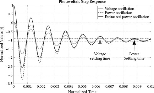
FIGURE 2.10
PV power dynamic behavior.

Evaluating the envelope of (2.17) in the T_ε yields

$\text{Δ}{P}_0\cdot \left(1+\text{ε}\right)\simeq \text{Δ}{P}_0\left(1-\frac{2}{\sqrt{1-{\zeta }^2}}\cdot e^{-{\text{ζω}}_{n}T\text{ε}}\right)$

(2.20)

so that the following expression of the settling time T_ε is obtained:

$T_{\text{ε}}\simeq -\frac{1}{\text{ζ}\cdot {\text{ω}}_n}\cdot ln\left(\text{ε}/2\right)$

(2.21)

It is worth noting that, with the same boundary value ε, the 1/2 factor in (2.21) makes the settling time of the PV power oscillation considerably different with respect to that of the PV voltage oscillation. For the example proposed in Figure 2.10, it is more or less 30% higher than the PV voltage settling time.

Based on the previous modeling results, the MPPT is not affected by mistakes caused by transient oscillations of the PV system caused by its own action if the following condition is fulfilled:

$T_p\ge T_{\int }\simeq -\frac{1}{\text{ζ}{\text{.ω}}_n}\cdot \ln {\left(\int ⁄2\right)|}_{\int =0.1}$

(2.22)

where the value ε = 0.1 is chosen according to the classical control system theory.

2.4.2    Rapidly Changing Irradiance Conditions

As discussed in Section 2.4.1, the perturbation period T_p should be set not much higher than the system settling time, in order to avoid instability of the MPPT algorithm and limit the oscillations across the MPP in steady state. The value to be assigned to the amplitude of the step perturbation Δx also requires a careful setting: A small value reduces the steady-state losses caused by the oscillation of the PV operating point around the MPP, but it makes the algorithm slower and less efficient in the case of rapidly changing irradiance conditions. The latter circumstance can deceive the P&O algorithm in MPP tracking [14]. Indeed, the possible failure of the P&O algorithm in the presence of varying irradiance may occur if the algorithm is not able to distinguish the variations of the PV power caused by the duty cycle modulation from those caused by the irradiance variation. An adequate choice of Δx can overcome this problem, as discussed in detail in this section.

Let us suppose that the system is working at the MPP in the k-th sampling instant (see Figure 2.11), at an irradiance level equal to G, and that the step perturbation Δx moves the operating point leftward, in the direction of lower array voltage, namely, from the MPP to point A in the absence of irradiation change. Let us then suppose that the irradiance level changes between the k-th and the (k + 1)-th sampling instants. In Figure 2.11 it has been assumed that it increases. Then the operating point at the (k + 1)-th sampling instant will be point B instead of point A.

Depending on the amplitude of Δx, two possible situations are possible, as shown in Figure 2.11. In the sequel the PV power variation (at a constant irradiance level G) caused by the perturbation of Δx triggered by the P&O algorithm will be named with ΔP_x, while ΔP_G identifies the PV source output power variation caused by the variation ΔG of the irradiance level. The P&O algorithm works properly if

$\left|\text{Δ}{\text{P}}_{\text{x}}\right|\ge \left|\text{Δ}{\text{P}}_{\text{G}}\right|$

(2.23)

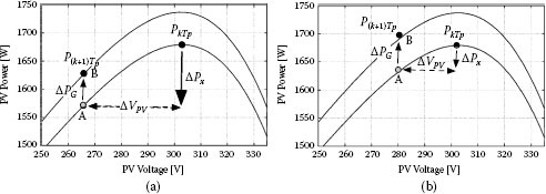
FIGURE 2.11
Operating point of PV field in the presence of an irradiance variation.

Condition 2.23 involves the absolute values because the signs of both power variations are not correlated and cannot be predicted in advance. For the case shown in Figure 2.11a, the inequality (2.23) is satisfied and the algorithm is not confused because it detects P_{(k + 1)Tp} < P_kTp, and consequently it will change the sign of the next perturbation, so that the operating point moves back to the MPP. In the case shown in Figure 2.11b, instead, the algorithm is confused because P_{(k + 1)Tp} > P_kTp, so that the next perturbation will have the same sign as the previous one; thus the operating point further moves in the direction of lower array voltage, away from the MPP.

Equation (2.23) can be made explicit by expressing each term as a function of the system parameters and PV field operating condition, so that the PV power variation is related to the Δx perturbation.

If the current and voltage variations with respect to the MPP are indicated as ΔI_PV and ΔV_PV, respectively, and if ΔP_PV = P_{(k + 1)Tp} − P_kTp is the whole power variation when the system moves from the MPP toward B (see Figure 2.11), then the following equations hold:

$V_B=V_{MPP}+\text{Δ}{V}_{PV}$

(2.24)

$I_B=I_{MPP}+\text{Δ}{I}_{PV}$

(2.25)

$\text{Δ}{P}_{PV}=P_B-P_{MPP}=V_{MPP}\cdot \text{Δ}{I}_{PV}+I_{MPP}\cdot \text{Δ}{V}_{PV}+\text{Δ}{V}_{PV}\cdot \text{Δ}{I}_{PV}$

(2.26)

ΔI_PV can be expressed as a function of ΔV_PV, but not by means of the linear relation (2.3) since ΔV_PV assumes large values. A quadratic expression is much more suitable and allows evaluaton, with an improved accuracy, of whether inequality (2.23) is verified or not.

$\text{Δ}{I}_{PV}\simeq {\frac{\partial i_{PV}}{\partial v_{PV}}|}_{MPP}\text{Δ}{V}_{PV}+\frac{1}{2}{\frac{{\partial }^2{i}_{PV}}{{\partial }^2{v}_{PV}}|}_{MPP}{\text{Δ}{V}_{PV}^2+\frac{\partial i_{PV}}{\partial G}|}_{MPP}{\text{Δ}G+\frac{\partial i_{PV}}{\partial T}|}_{MPP}\text{Δ}{T}_a$

(2.27)

In (2.27) the PV current variation with respect to the irradiance variation ΔG has been considered only with the first derivative term because at the MPP the current variation is almost linear with respect to ΔG, as shown in [11]. Although in (2.27) the effect of the ambient temperature variation is also considered, in the following ΔT_a ≃ 0 will be considered, because in the short time interval between two perturbations (T_p), the PV operating temperature can be assumed constant.

The partial derivative of the PV current can be evaluated as follows:

$\frac{1}{2}{\frac{{\partial }^2{i}_{PV}}{{\partial }^2{v}_{PV}}|}_{MPP}=-H$

(2.28)

$H=\frac{1}{2}\frac{1}{\text{η}{V}_t}{\left(1-\frac{R_s}{R_{MPP}}\right)}^3\left(\frac{I_{sat}}{\text{η}{V}_t}{e}^{\frac{V_{MPP}+R_s{I}_{MPP}}{\text{η}{V}_t}}\right)$

(2.29)

where R_s, V_t, and I_sat are the values of the parameters of the model describing the whole PV generator. The term related to the irradiance variation is given by

$\frac{\partial i_{PV}}{\partial G}\simeq \frac{\partial i_{ph}}{\partial G}=K_{ph}$

(2.30)

where K_ph is a PV material constant [11] that can be evaluated by using Equation (1.2).

By means of (2.11), the PV current variation is expressed as follows:

$\text{Δ}{I}_{PV}\simeq -\frac{\text{Δ}{V}_{PV}}{R_{MPP}}-H\cdot \text{Δ}{V}_{PV}^2+K_{ph}\cdot \text{Δ}G$

(2.31)

On the basis of (2.26), (2.31), and (2.12), the PV power variation can be rewritten:

$\text{Δ}{P}_{PV}\simeq -\left(H\cdot V_{MPP}+\frac{1}{R_{MPP}}\right)\cdot \text{Δ}{V}_{PV}^2+V_{MPP}\cdot K_{ph}\text{Δ}G$

(2.32)

where in (2.32) the higher-order terms have been neglected.

The effect of the Δx step perturbation on the corresponding steady-state variation ΔV_PV of the array voltage is evaluated by using the transfer function G_vp,x(s) introduced in section 2.4.1:

$\text{Δ}{V}_{PV}=G_0\cdot \text{Δ}x$

(2.33)

where G₀ is the DC gain of G_vp,x(s).

If Δx is the only stimulus that triggers the PV voltage variation, then

$\left|\text{Δ}{P}_x\right|=\left(H\cdot V_{MPP}+\frac{1}{R_{MPP}}\right)\cdot G_0^2\cdot \text{Δ}{x}^2$

(2.34)

$\left|\text{Δ}{P}_G\right|=V_{MPP}\cdot K_{ph}\cdot \left|\text{Δ}G\right|=V_{MPP}\cdot K_{ph}\cdot \left|\dot{G}\right|\cdot T_p$

(2.35)

where $\dot{G}$ is the average rate of change of the irradiance level inside the period of the MPPT perturbation T_p occurring between the k-th and the (k + 1)-th sampling instants.

Under the hypotheses adopted above, the inequality (2.23) is fulfilled if the following condition is fulfilled by the Δx amplitude:

$\text{Δ}x>\frac{1}{G_0}\sqrt{\frac{V_{MPP}\cdot K_{ph}\cdot \left|\dot{G}\right|\cdot T_p}{\left(H\cdot V_{MPP}+\frac{1}{R_{MPP}}\right)}}=\text{Δ}{x}_{min}$

(2.36)

Setting the values of T_p and Δx on the basis of Equations (2.21) and (2.36), respectively, ensures that the P&O algorithm is able to track, without errors, irradiance variations characterized by an average rate of change (within T_p) not higher than $\dot{G}$.

It is worth noting that the parameters H, V_MPP, and R_MPP depend on the irradiance level. Thus when using the (2.21) and (2.36) design equations, the combination of parameters (H, V_MPP, R_MPP) leading to the highest value of the T_p and Δx parameters must be used. In the next section a design example is proposed in order to show how to apply the proposed MPPT design procedure.

2.4.3    P&O Design Example: A PV Battery Charger

Guidelines for designing the P&O algorithm based on the duty cycle perturbation are analyzed in this section. Figure 2.12 shows the basic scheme of a PV battery charger based on a boost DC/DC converter. An additional control circuitry, providing battery over voltage and over current protections, which must be considered in the practical application, has no effect on the MPPT design procedure.

As explained in Section 2.4.1, the first step is to identify the control-to-PV voltage transfer function: In the case under study the MPPT acts on the duty cycle directly so that $G_{vp,x}\left(s\right)={\widehat{v}}_{PV}/\widehat{x}$ corresponds to $G_{vp,d}\left(s\right)={\widehat{v}}_{PV}/\widehat{d}$. The scheme of Figure 2.13 shows the whole small-signal model of the PV battery charger that can be used to evaluate G_vp,d(s).

As steady-state environmental conditions are supposed, the small-signal model of the PV field is given by its differential resistance obtained by using (2.5) in the MPP. The DC/DC converter, instead, is decoupled in its linear parts and in a linearized small-signal part [12] modeled by the following equations:

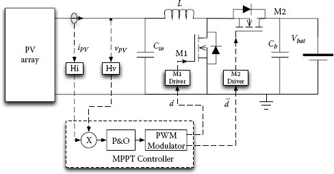
FIGURE 2.12
PV battery charger with a boost converter.

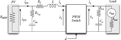
FIGURE 2.13
Small-signal model of PV battery charger.

$\{\begin{array}{l}{\widehat{i}}_2=\left(1-D\right)\cdot {\widehat{i}}_1-I_1\cdot \widehat{d}\\ {\widehat{v}}_1=\left(1-D\right)\cdot {\widehat{v}}_2-V_2\cdot \widehat{d}\end{array}$

(2.37)

which completely describe the block PWM SWITCH shown in the scheme of Figure 2.13 and deeply analyzed in [12]. The additional small-signal source ${\widehat{v}}_{bat}$ is used to model the low-frequency variations at the converter’s output caused by load changes.

The oscillations ${\widehat{v}}_{bat}$ can propagate up to the PV terminals, thus causing a possible deceiving effect on the operation of the MPPT algorithm, because it might be unable to distinguish the PV voltage oscillations caused by ${\widehat{v}}_{bat}$ with respect to the PV voltage oscillations introduced by the perturbation of the duty cycle $\widehat{d}$. In this example the battery is considered an ideal voltage source; thus ${\widehat{v}}_{bat}=0$, R_bat = 0. The problems related to the disturbances coming from the converter output will be investigated in depth in Chapter 3.

In this example the main parasitic parameters of the DC/DC converter have been also accounted for; nevertheless, G_vp,d(s) assumes an expression similar to (2.15):

$G_{vp,d}\left(s\right)=\frac{\text{μ}\cdot {\text{ω}}_n^2\cdot \left(1+\frac{s}{{\text{ω}}_z}\right)}{s^2+2\text{ζ}\cdot {\text{ω}}_n\cdot s+{\text{ω}}_n^2}$

(2.38)

where

$\text{μ}=-V_{bat}{\text{ω}}_n=\frac{1}{\sqrt{L\cdot C_{in}}}{\text{ω}}_z=\frac{1}{R_{C_{in}}\cdot C_{in}}$

(2.39)

$\text{ζ}=\frac{1}{2\cdot R_{MPP}}\sqrt{\frac{L}{C_{in}}}+\frac{R_{C_{in}}+R_L}{2}\sqrt{\frac{C_{in}}{L}}$

(2.40)

FIGURE 2.14
Settling time evaluation for the PV battery charger.

The high-frequency zero appearing in the G_vp,d(s) transfer function, which has been introduced by the resistance R_Cin, does not affect significantly the transient; thus the MPPT analysis can be carried out by using (2.22). If the transfer function assumes a more complex form, it is always possible to estimate the settling time T_ε numerically or graphically by evaluating the time response of the PV voltage for a step duty cycle perturbation. Typical waveforms of the PV voltage oscillation for different irradiance conditions have been shown in Figure 2.14.

The values of the parameters of the boost converter are reported in Table 2.1, and those concerning the PV module have been reported in Table 1.3, where more realistic outdoor environmental conditions have been considered. The damping factor ζ depends on the PV differential resistance R_MPP, which is strongly related to the irradiance level; thus in the evaluation of the parameters of the MPPT controller, the worst-case conditions must be considered.

The continuous line in Figure 2.14 has been obtained by considering an irradiance level of G = 1000 W/m², and the corresponding differential resistance is given by R_MPP|G=1000≃ 11Ω. The dashed line is the PV voltage transient for an irradiance level of G = 100 W/m², which corresponds to R_MPP|G=100≃ 11Ω. In the analysis and characterization of dynamic systems, ε = 0.1 is usually assumed as a reasonable threshold to consider the transient over; thus the PV power settling times, evaluated by means of (2.21), are, respectively, T_ε|_G=1000≃ 0.5ms and T_ε|_G=100≃ 2.3ms. Such values are approximately the same marked on the plots of Figure 2.14, where the settling time has been evaluated by analyzing the PV voltage oscillations.

According to (2.22), in order to ensure the right behavior for the P&O algorithm, the minimum value of T_p must be chosen higher than 2.3 ms.

TABLE 2.1

Parameters and Nominal Operating Conditions for the PV Battery Charger

Boost Parameters	Nominal Values
Input capacitance Cin	110 μF
Equivalent series resistance of Cin	5 mΩ
Output capacitance Cout	2 × 22 μF
Inductance L	13.8 μH
Equivalent series resistance of L	20 mΩ
Operating Conditions	Nominal Values
Switching frequency fs	200 kHz
PWM gain modulator (Vm)	1 V
Battery voltage Vbat	12 V
Voltage sensor gain Hv	1
Current sensor gain Hi	1 V/A

The behaviors of the PV array voltage and of the duty cycle for different P&O parameters values have been shown in Figure 2.15. Figure 2.15a refers to a simulation of the circuit in Figure 2.12 by using an MPPT perturbation period T_p = 1 ms, while results shown in Figure 2.15b have been obtained with T_p = 2.5 ms. In order to test different environmental conditions, for both simulations, at the time instant t = 30 ms the irradiance changes from 1000 W/m² to 100 W/m².

For an ideal system operating in steady-state environmental conditions, the P&O step amplitude, which corresponds to Δx = Δd for the MPPT algorithm acting on the duty cycle, does not affect the behavior of the MPPT algorithm. More in general, as the switching converter intrinsically generates the noise due to the switching ripple on the sensed variable, a minimum value for Δd must be selected in order to overcome such disturbances*:

$\text{Δ}{V}_{P{V}_{\text{Δ}d}}=Go\cdot \text{Δ}d>\text{Δ}{V}_{P{V}_{ripple}}$

(2.41)

where ΔV_PVΔd is the PV voltage variation due to the perturbation Δd and ΔV_PVripple is the amplitude of the switching ripple on the PV voltage.

In the boost-based battery charger configuration, if no additional filter is used for removing the switching ripple noise, the minimum Δd can be estimated by using the following condition:

$\text{Δ}d>\frac{\left(V_{bat}-V_{MPP}\right)\cdot V_{MPP}}{16\cdot L\cdot C_{in}\cdot f_s^2\cdot V_{bat}^2}$

(2.42)

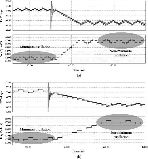
FIGURE 2.15
P&O behavior in steady-state environmental conditions.

For the operating conditions considered in the case under study, applying (2.42) provides Δd > 0.001. A P&O step amplitude Δd = 0.005 has been used for the tests whose results are shown in Figure 2.15.

As shown in the two plots, for t < 30 ms, the MPPT works correctly because T_p is greater than T_ɛ|G=1000 = 0.5ms: In this case, the P&O algorithm is not confused by the transient behavior of the system and the duty cycle oscillates assuming only three different values: [d_MPP − Δd,d_MPP,d_MPP + Δd]

For t > 30 ms, the first simulation highlights that the P&O algorithm is not able to work with only three steps; in fact, in this case T_p = 1ms < T_ɛ|G=100 = 2.3ms and the operating point has a wider swing across the MPP, and then the system is characterized by a lower efficiency with respect to the corresponding case (T_p = 2.5 ms) shown in Figure 2.15b. In this second case, after a transient necessary to adapt the system to the new environmental conditions, the P&O continues to work correctly because T_p fulfills the constraint (2.22) for all operating conditions tested in the example.

As discussed in Section 2.4.2, once given the maximum $\dot{G}$ to be tracked without error, the optimal value of Δd can be settled. This is an important aspect conditioning the MPPT performances, especially on a cloudy day, when the PV field is subject to continuous irradiance change and a wrong MPPT configuration can significantly reduce the energy efficiency of the system.

It is very important to adopt a realistic characterization of the performances together with the analysis of the balance of the system related to power components adopted, for a reliable estimation of PV systems energy productivity and economic convenience. Some interesting considerations about such aspects are reported in [15], where an overview of the EN 50530, which is the European standard for measuring the overall efficiency of PV inverters, is provided. The document explains in depth the approach and methodology introduced in the standard for a combined assessment of the conversion as well as the maximum power point tracking efficiency. In particular, the dynamic MPPT efficiency under varying irradiance conditions is identified by using a ramp sequence consisting of irradiance ramps with different gradients as well as irradiance levels.

In detail, ramp gradients ranging from $\dot{G}=0\cdot 5W/m^2/s$ to $\dot{G}=100W/m^2/s$ are used for the tests with two different irradiance levels, from 100 W/m²/s to 500 W/m² (low to medium irradiance) as well as from 300 W/m²/s to 1000 W/m² (medium to high irradiance). On the basis of the indication given in the standard, for the example under study, a constant rate of change for the irradiance variation $\dot{G}=100W/m^2/s$ is considered. The worst-case conditions of G = 100 W/m² will be considered for estimating the parameters that are used in Equation (2.36) for evaluating the right Δd step amplitude.

By means of (2.29), with the data reported in Tables 1.2 and 1.3, the parameter H|_{G = 100} = 0.0836 A/V2 has been obtained. Finally, applying (2.36) for the step amplitude Δd provides

$\text{Δ}d>\frac{1}{V_{bat}}\sqrt{\frac{V_{MPP}\cdot K_{ph}\cdot \left|\dot{G}\right|\cdot T_p}{\left(H\cdot V_{MPP}+\frac{1}{R_{MPP}}\right)}}\simeq 0.0118$

(2.43)

where the K_ph variable assumes the following value: K_ph = 0.008 A·m²/W.

Figure 2.16 shows the behavior of the PV system in the presence of irradiance variations. The irradiance profile characterized by a positive and negative ramp with a slope of ± 100 W/m²/s, as shown in Figure 2.16a, has been used in the simulation. The P&O algorithm with the optimal values of T_p = 2.5 ms and Δd = 0.012, selected according to Equation (2.43), has been compared with another case in which Δd = 0.0012 has been used. In Figure 2.16b the duty cycle waveforms of the two cases have been superimposed. The simulation shows that if the amplitude of the duty cycle perturbation is well designed, also in the presence of irradiance variation, the duty cycle oscillates assuming only three different values.

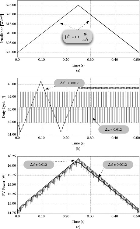
FIGURE 2.16
P&O behavior in dynamic environmental conditions. (a) Irradiance profile. (b) Duty cycle variations. (c) Instantaneous PV power.

In Figure 2.16c the instantaneous power, delivered by the PV source, has been plotted for the two MPPT controllers. The simulation highlights that the optimal Δd, which is one order of magnitude greater than the minimum values required for the steady-state conditions, ensures highest efficiency because the MPPT is not deceived in the tracking process.

For the proposed example, the design setup has also been experimentally validated. In Figure 2.17 the simulation waveforms of the PV battery charger (Figure 2.17a) and the oscilloscope waveforms (Figure 2.17b) of the photovoltaic voltage and current have been shown. The comparison is totally satisfactory and the MPPT P&O algorithm works as predicted by moving the operating point in only three positions around the MPP.

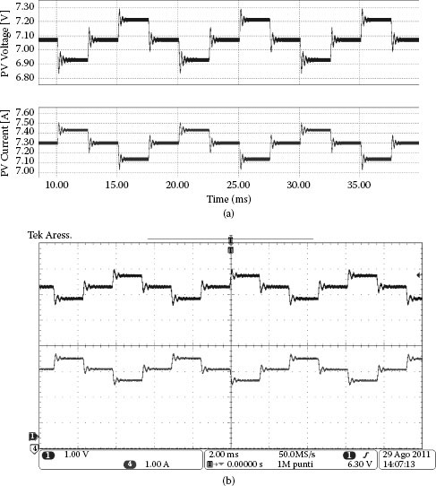
FIGURE 2.17
Experimental test of the MPPT for battery charger. (a) Simulation results. (b) Experimental results.

2.5    Improvements of the P&O Algorithm

2.5.1    P&O with Adaptive Step Size

The P&O algorithm is widely used in PV systems due to its simplified control structures and easiness of implementation. In the MPPT algorithm with fixed {Δx, Tp} parameters a trade-off condition must be achieved in order to choose the controller values for balancing the losses in steady state due to large perturbations around the MPP and the MPPT speed in situations involving quickly changing irradiation conditions or load.

In the previous paragraphs, benefits deriving from the optimization of both the perturbation amplitude Δx and the sampling period T_p have been shown. Nevertheless, overall MPPT performances can be further improved by modifying the basic version of the Hill climbing and P&O algorithms.

For example, in [16], a method in which the duty cycle step size is automatically adjusted according to the derivative of power with respect to the PV voltage (dP/dV) is proposed. The step size becomes tiny as dP/dV becomes very small around the MPP, thus ensuring a very good accuracy at steady state. In such a cases the general equation (2.2) is modified as follows:

$d_{\left(\left(k+1\right)T_p\right)}=d_{\left(k{T}_p\right)}\pm \text{Δ}d=d_{\left(k{T}_p\right)}\pm N\cdot \frac{\left|P_{\left(k{T}_p\right)}-P_{\left(\left(k-1\right)T_p\right)}\right|}{\left|V_{P{V}_{\left(k{T}_p\right)}}-V_{P{V}_{\left(\left(k-1\right)T_p\right)}}\right|}$

(2.44)

where N is the scaling factor adjusted at the sampling period to regulate the step size. In [17], the variable step size algorithm is implemented according to the slope of the PV power vs. the duty cycle curve on the basis of the following relation:

$d_{\left(\left(k+1\right)T_p\right)}=d_{\left(k{T}_p\right)}\pm \text{Δ}d=d_{\left(k{T}_p\right)}\pm N\cdot \frac{\left|P_{\left(k{T}_p\right)}-P_{\left(\left(k-1\right)T_p\right)}\right|}{\left|d_{\left(k{T}_p\right)}-d_{\left(\left(k-1\right)T_p\right)}\right|}$

(2.45)

The performance of the algorithm (2.44) and Equation (2.45) is essentially conditioned by the scaling factor N. The manual adjustment of the value of this parameter is often based on a trial-and-error approach, and the value resulting from this process is just suitable for a given system and specific operating conditions.

In order to ensure the convergence of the MPPT algorithm, the parameter N must meet the following inequality [17]:

$N\cdot \frac{\left|\text{Δ}{P}_{max}\right|}{\left|\text{Δ}{V}_{max}\right|}<\text{Δ}{d}_{max}$

(2.46)

where Δd_max is the maximum desired step change. In [17] an experimental procedure aimed at identifying the best value for N is proposed. At the startup, the duty cycle d_start is initialized at a low value. Power p_start and voltage v_start are evaluated with such duty cycle value. Afterwards, the duty cycle value is modified by the maximum desired step change Δd_max and corresponding values of ΔP_max and ΔV_max are evaluated. Equation (2.46), which provides a guide to determine the value of the scaling factor N, can be used in conjunction with (2.36), so that the largest step size of an equivalent fixed step size MPPT algorithm is evaluated by assuming the worst-case operating conditions.

The value of the perturbation period T_p must be designed according to (2.22). The algorithm is explained by means of Figure 2.18: The initial operating point is assumed to be x₁ and the perturbation step size is assumed to be step 1. The sequence x₁–x₇ is obtained by imposing an amplitude of the perturbation proportional to the variation of the PV power.

2.5.2    P&O with Parabolic Approximation

In [18] it is shown that a parabolic interpolation based on the last three sampled voltage-power couples allows us to balance the position of the three operating points across the MPP. The unbalanced position of the operating points across the MPP, which can occur if any perturbative MPPT approach is used, has a detrimental effect on the MPPT efficiency, and thus it must be corrected properly.

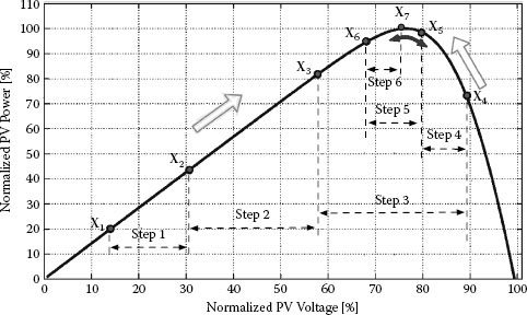
FIGURE 2.18
Variable step MPPT.

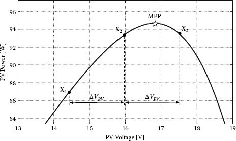
FIGURE 2.19
Operating points location on PV characteristic.

In a fixed step size P&O algorithm, the discretized value of Δx usually does not allow us to have a three-point steady-state behavior with a central point close to the MPP and the other two equally balanced at its sides. A very common situation is that shown in Figure 2.19, where the operating points x₁, x₂, and x₃ are equally spaced in terms of PV voltage, but they are not well balanced with respect to the MPP.

The lower Δx, the lower the distance between x₂ and the MPP. The non-symmetrical position of the three operating points is less efficient than the balanced condition, occurring when x₂ is centered in MPP with x₁ and x₃ equally spaced in terms of PV voltage, and it might also trigger a four-point oscillation, with a further increase of the power loss. A four-point oscillation obtained in an experimental case is shown in Figure 2.20. A sequence of seven operating points around the MPP of the P&O algorithm is plotted. If the position of the operating points is asymmetric with respect to the MPP, the points that are closer to the MPP (x₂ and x₃ in Figure 2.19) have more or less the same power level. In the presence of noise and rounding errors introduced by the measurement system, the action of the MPPT algorithm might be wrong. For instance, when the operating point jumps from position 5 to 6, due to noise or slight variations of the irradiance level, the measured value of the PV power might be different from that evaluated in point 2. As a consequence, ΔP has a sign that causes an additional step in the wrong direction (1 = 7). By comparing the real sequence (1-2-3-4) with respect to the optimal three-point oscillation (1-2-3) or (2-3-4), the difference in terms of power losses is almost evident. It will be quantified in Section 2.8.

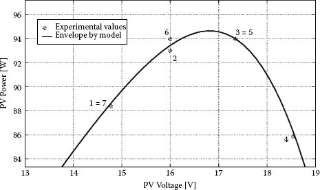
FIGURE 2.20
Steady-state oscillations in a noisy environment.

If one of the points 2 or 3 is moved much closer to the MPP, the errors are less significant than the power variation due to the jump from one operating point to the following one. This aspect is explained with the support of Figure 2.21 and by considering the relative position of the operating point with respect to the power variation.

In Figure 2.21a the power variation (ΔP) between two possible operating points across the MPP has been put into evidence. In the presence of an uncertainty u_ΔP due to the measurement process, the result can be affected by an error higher than the nominal value, so that u_ΔP > ΔP. Due to the concavity of the curve at the MPP, regardless of the step amplitude, the case ΔP ≃ 0 can occur, with a consequent wrong decision of the MPPT algorithm.

Figure 2.21b shows the case of a balanced configuration, obtained by moving forward the operating points without changing the Δx value. After this shift, the system works correctly because it is ΔP > uΔP for any operating condition.

Some tricks have been proposed in literature for addressing the problem described above. In [19], a memory buffer containing the last three PV voltage-power couples is employed for detecting if the MPP has been reached and if a rapid irradiation variation occurs. The importance of freezing the value of the converter duty cycle when the MPP is reached is also put into evidence: This allows us to draw the maximum power in steady-state conditions without missing any part of it due to the oscillations around the MPP. In [20], and in some other papers reported in the list of references cited therein, the basic P&O MPPT technique is compared with some improved versions. Some of them suggest the use of a waiting function aimed at freezing the duty cycle perturbation value if the sign of Δd is reversed several times in a row. This trick reduces the hill climbing of the operating point across the MPP under stationary irradiance conditions, but it deteriorates the system response under changing atmospheric conditions. This emphasizes the P&O erratic behavior under rapidly changing irradiance conditions typical of cloudy days.

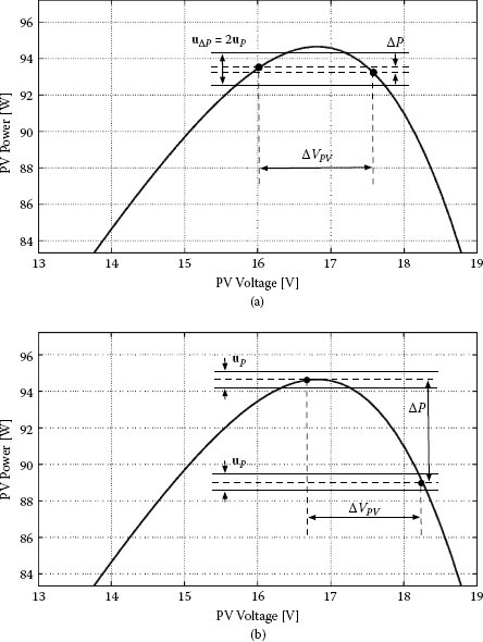
FIGURE 2.21
Balancing the steady-state oscillations for error compensation. (a) Two points with similar power. (b) Two points well displaced on the PV curve.

Among the techniques proposed in literature, the balancing of the steady-state operating points across the MPP by employing a parabolic interpolation is very effective and relatively simple. Indeed, near the MPP, the parabola is a good approximation of the P-V curve; thus it can be used for estimating the position of the MPP by using the information coming from the last three operating points [18, 21].

A parabola is described in the P-V plane by the following equation:

$p_{PV}=\text{α}\cdot v_{PV}^2+\text{β}\cdot v_{PV}+\text{γ}$

(2.47)

with α < 0 and the vertex at v_peak = − β / (2α), with p_peak = γ − β²/(4α)

If the P-V curve and the interpolating parabola have at least three points in common, the coefficients α, β, and γ can be determined by solving the following system of equations:

$\{\begin{array}{l}{p}_1=\text{α}\cdot v_1^2+\text{β}\cdot v_1+\text{γ}\\ p_2=\text{α}\cdot v_2^2+\text{β}\cdot v_2+\text{γ}\\ p_3=\text{α}\cdot v_3^2+\text{β}\cdot v_3+\text{γ}\end{array}$

(2.48)

A first-in/first-out array containing the actual operating point and the preceding two, corresponding to the couple of values [(p₁,v₁) − (p₂,v₂) − (p₃,v₃)], is used to find the interpolating parabola. Once such an approximation is obtained, the vertex of the parabola is used as a prediction of the new operating point, as shown in Figure 2.22.

The interpolating parabola is considered misleading in the MPPT process if it exhibits an upward-turned concavity, or if it has a vertex at a voltage higher than the open-circuit voltage, as in Figure 2.23. In such cases, as well as if it cannot be found by means of the three points given (e.g., when two of them are superimposed), the perturbation used by the P&O algorithm is that one determined by means of (2.36).

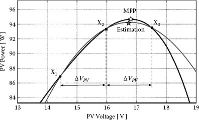
FIGURE 2.22
MPP estimation by means of parabolic (red curve) interpolation.

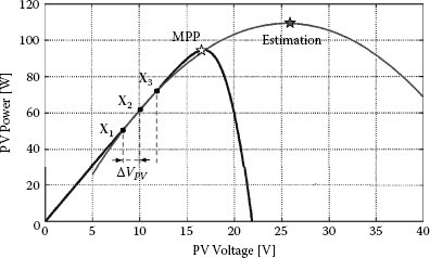
FIGURE 2.23
Wrong estimation of parabolic interpolation.

The promptness of the MPPT controller is also improved by exploiting the geometrical properties of the parabolic function. A sequence of the PV operating points is shown in Figure 2.24: By assuming that the MPPT controller starts to work with a fixed step size ΔV_PV, after two steps the values x₁, x₂, and x₃ are available for reconstructing the interpolating parabola. If the estimated step amplitude ΔV_parabolic is higher than ΔV_PV, the MPPT algorithm can reach the MPP in a few steps. In [18] details concerning the performance in the presence of irradiance variations and more information related to the practical implementation of the parabolic approach are provided.

2.6    Evolution of the Perturbative Method

2.6.1    Particle Swarm Optimization (PSO)

Particle swarm optimization (PSO) has also been proposed as an MPPT approach, especially because it is not computationally burdensome. PSO allows implementation by means of low-cost digital controllers and is characterized by good performance under extreme irradiation conditions. In [22] the authors propose a modification of a classical perturbative approach, directly applied to the duty cycle of a DC/DC converter, based on a PSO method. The main objective of the study is to achieve a strong reduction, or even the absence, of the steady-state oscillations around the MPP that are a drawback of any perturbative MPPT technique. The PSO algorithm is seen as a perturbative method with an adaptive amplitude of the applied perturbation. The particle velocity has been designed so that its value is close to zero when the system operation approaches the MPP and the value of the DC/DC converter duty cycle is approaching a constant. The application of the method requires a tuning of some parameters that strongly affect performances, some of them being dependent on the specific application. In [22] it has also been demonstrated that PSO is effective in tracking the MPP when the PV generator is affected by partial shadowing phenomena.

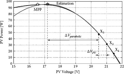
FIGURE 2.24
Promptness MPPT improvement by means of parabolic interpolation.

In [23] the authors apply a PSO algorithm to the problem of PV arrays working in mismatched conditions. The approach proposed by the authors is not based on the assumption that the mismatched PV panels are still connected in series so that the power vs. voltage curve of the string exhibits more than one maximum power point. In particular, the authors adopt a centralized MPPT controller, running the PSO, acting on the duty cycle of as many DC/DC converters as the PV panels in the string. Such an approach is also proposed in [24], where the authors use the same architecture with a different control algorithm. The multivariable optimization algorithm proposed in [23] adjusts the converter’s duty cycle values with the aim of maximizing the total power delivered at the output. Only three agents allow tracking of the absolute MPP; however, some parameters (e.g., the one defining the convergence criterion and the one introduced for detecting an irradiation change) must be designed carefully, according to the real case under analysis, if high tracking performances are required.

2.6.2    Extremum Seeking and Ripple Correlation Techniques

Extremum seeking (ES) control is always confused with the ripple correlation control (RCC) technique. Their applications to the MPPT problem are very similar, the true difference being the source of perturbation used to detect whether the PV array is operating on its MPP or is on the right or left side of the MPP itself. As clearly explained in [25], ES adopts a signal having a low-frequency oscillating component and RCC employs the ripple at the switching frequency generated by the power electronic circuit, so that this is able to fasten the RCC convergence.

In PV MPPT single-phase AC applications, ES can use the oscillating component at 100 or 120 Hz, depending on the frequency of the AC voltage, which can be 50 or 60 Hz, for tracking the MPP. As will be shown in Chapter 3, such an oscillation appears at the DC bus connecting the DC/AC inverter with the DC/DC converter performing the MPPT function in double-stage topologies. Such an oscillation back propagates through the DC/DC converter and, as will be shown in Chapter 3, worsens the performances of the MPPT algorithm. Nevertheless, it can be used for tracking the maximum power point. Alternatively, e.g., in DC applications, a sinusoidal low-frequency disturbance can be even injected for accomplishing the same work, but at the price of additional circuitry. The operating principle is explained in Figure 2.25.

The sinusoidal disturbance affects the PV voltage and has an effect on the PV power. This effect is almost negligible if the operating point voltage is the MPP. If the PV array is working at a voltage lower than the MPP one, the oscillation affecting the PV power is in phase with that imposed on the PV voltage. On the contrary, at any voltage higher than MPP one, the PV power oscillation is displaced by half a period with respect of the voltage oscillation. Figure 2.26 shows that a sinusoidal external dither is superimposed on the PV voltage. The PV power frequency component at the same frequency of the injected signal is multiplied by the latter one, and the average value of the product has a sign that can drive the MPPT toward the peak of the P-V function [26].

Figure 2.27 shows that once the sinusoidal disturbance takes place at the PV terminals due to the DC/AC stage, the demodulated signal to be processed by the low-pass filter is obtained by multiplying the oscillations affecting both the PV power and the PV current [27]. The employment of the inherent oscillations of the instantaneous power in single-phase systems is also proposed in [28], where the authors propose a suitable filtering of the PV current and voltage signals allowing an estimation of the PV power derivative. A suitable control of the DC link voltage allows us to perform the MPPT operation.

Also, in the case of ripple correlation control (RCC), the time derivative of the power is related to the time derivative of the current or of the voltage, but no external oscillation is required. The power gradient is driven to zero by using the natural ripple that occurs due to converter high switching frequency [29]. In this way, the RCC method can also be used in PV applications with DC loads or battery chargers as well as three-phase loads or grid connection.

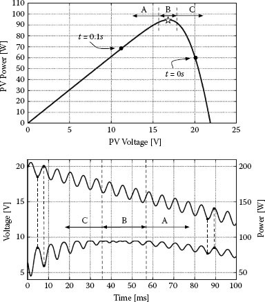
FIGURE 2.25
Principle of operation of the ES control algorithm.

In [30] the RCC technique is improved furthermore, because the study of the wave shapes of the electrical variables in the switching converter has allowed us to reduce the requirements in terms of sampling. In fact, only two samples per switching period, one taken at the minimum value of the PV current, that is, the maximum for the PV voltage, and the second taken at its maximum, which is the minimum for the PV voltage, are needed.

2.6.3    The Incremental Conductance Method

This method was first presented in [31], and it is based on the observation that in the MPP, the following condition occurs:

$\frac{dP}{dV}=\frac{d\left(V\cdot I\right)}{dV}=0$

(2.49)

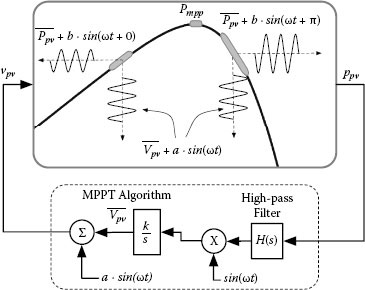
FIGURE 2.26
ES MPPT by an external dither.

By accounting for the dependence of the PV current on the voltage, it is possible to express such a condition as follows:

$I+V\cdot \frac{dI}{dV}=0$

(2.50)

so that the validity of condition (2.49) is equivalent to

$\frac{I}{V}=-\frac{dI}{dV}$

(2.51)

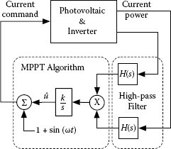
FIGURE 2.27
ES MPPT using the low-frequency oscillation produced by an inverter stage.

which means that, at the MPP, the absolute value of the conductance must be equal to the absolute value of the incremental conductance. Such a condition is the basis of the incremental conductance (INC) MPPT method. Condition (2.51) is verified through a repeated measure of the conductance at two different, yet close enough, values of the PV voltage. As a consequence, the method requires the application of a repeated perturbation of the voltage value, until the following condition occurs:

$\frac{I_k}{V_k}=-\frac{I_k-I_{k-1}}{V_k-V_{k-1}}$

(2.52)

where the indices k and k − 1 refer to two consecutive samples of the PV voltage and current values. In [31] an 8.4% increase in the PV power produced by a PV system equipped with the INC MPPT method is claimed with respect to the P&O method. The reason for this improvement has been mainly ascribed to the fact that the INC method is able to avoid any further oscillation of the operating point when condition (2.52) has been fulfilled. Consequently, the INC method behaves in a way that is similar to P&O during transients, but it is able to avoid any power loss in steady-state conditions because it remains in the MPP unless any exogenous variable makes (2.52) no more fulfilled.

Unfortunately, condition (2.52) holds only for an ideal system, because it is almost never verified because of noises and quantization effects, related to the microcontroller by means of which the INC method is implemented. As a consequence, the method continues to check the validity of (2.52) also in stationary irradiance conditions, so that the theoretical advantage of INC over P&O vanishes.

The evaluation of (2.52) can be useful in order to understand on which side of the P-V curve with respect to the MPP the actual operating point lies. Indeed, by means of (2.49) and (2.50) we get

$\frac{1}{V}\cdot \frac{dP}{dV}=\frac{I}{V}+\frac{dI}{dV}=G+dG$

(2.53)

where G is the conductance and dG the incremental conductance. It results that, on the left side of the P-V curve with respect to the MPP, dP/dV > 0: This means, according to (2.53), that G + dG > 0. As a consequence, if the conductance is greater than the absolute value of the incremental conductance, than the operating point is on the left side of the MPP, so that the voltage must be increased in order to move closer to the MPP. Similarly, if G + dG < 0, the actual operating point is at a voltage higher than that of the MPP, so that the voltage must be reduced if the MPP has to be approached. Such information is not available if the P&O technique is used, so this is a real advantage ensured by the INC method. The new voltage at which condition (2.51) must be tested is evaluated according to the following iterative formula:

$V_{PV}^{k+1}=V_{PV}^k+sign\left(G+dG\right)\cdot \text{Δ}V$

(2.54)

where ΔV is the voltage step chosen for the perturbative phase during which the MPP is searched. The flowchart shown in Figure 2.28 puts into evidence the perturbative nature of the INC algorithm and the use of the information deriving from the comparison between the values of the conductance and the incremental conductance.

Due to fact that the INC method is inherently based on a perturbative approach, the amplitude of the perturbation step needs to be optimized as for the P&O, regardless of whether it acts on the duty cycle or on the reference voltage. In [32] a direct dependency of the step amplitude on the power derivative has been used. The formula proposed therein is referred to as direct control of the converter’s duty cycle.

$\text{Δ}D=\pm N\cdot \left|\frac{dP}{dV}\right|$

(2.55)

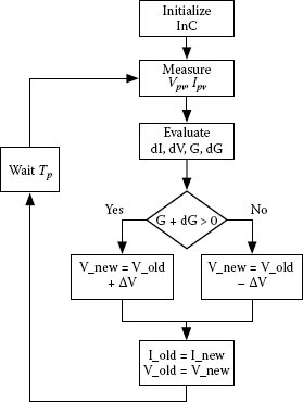
FIGURE 2.28
Flowchart of the incremental conductance algorithm.

In this way, the lower the power derivative, the closer is the MPP and the smaller the duty cycle perturbation that can be settled. The authors also propose an upper bound for the value of the coefficient N, which affects the tracking performances dramatically. The inequality involves the power derivative obtained at the larger ΔD to be used, and the value thereof and its meaning are the same as in (2.46).

$N<\frac{\text{Δ}{D}_{max}}{{\left|\frac{dP}{dV}\right|}_{fixedstep=\text{Δ}{D}_{max}}}$

(2.56)

Dynamic performances under very fast irradiation variation are claimed to be improved in [33], where a suitable function used for the MPP bounding is introduced. The algorithm step size modes are switched by the extreme values of a threshold function that is the product of the n-th power of the PV array output power and the derivative of the same power:

$C=P^n\cdot \left|\frac{dP}{dI}\right|$

(2.57)

the parameter n being used for a closer MPP bounding. The function C has two maximum values, for two different current values, one on the left side and one on the right side of the MPP. The proposed MPPT algorithm uses a variable step size mode if the PV array current falls between these two current values. Otherwise a fixed step size mode is used. This method improves both the steady state and the dynamic MPPT response.

2.7    PV MPPT via Output Parameters

The MPPT operation can be achieved by using the DC/DC converter output voltage and current rather than the input ones. The adoption of the output variables simplifies the MPPT algorithm. Moreover, regardless of the power stage and the way the control algorithm is implemented, this approach needs the sensing of only one of the two output variables. Indeed, it has been demonstrated that the MPPT using one output control parameter applies to almost any practical load type, regardless of its nature. Tracking the maximum value of the load current or voltage implies operation of the PV system at its MPP [34]. The controller simplicity translates into a reduction in the hardware involved, in terms of sensors, and in a MPPT algorithm that does not require the multiplication needed for the calculation of the PV power. It should be noted that in the majority of practical PV systems with battery backup, the DC/DC converter output voltage and current are monitored anyway, for the sake of charge control and battery protection. Thus the sensing of the PV array output voltage and current is avoided with benefits in terms of cost, system efficiency, and reliability. In [35] the design guidelines proposed in the previous paragraphs have been applied to the scheme of Figure 2.29.

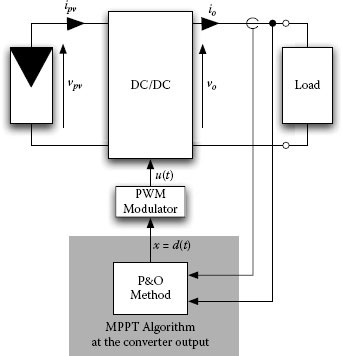
FIGURE 2.29
MPPT scheme via output parameters.

2.7.1    The TEODI Approach

A new MPPT technique based on the converter output parameters has been recently presented in the literature: It is named TEODI [36,37,38]. TEODI is the acronym used to synthesize the following concept: technique based on the equalization of the output operating points in correspondence of the forced displacement of the input operating points of two identical PV systems.

The main advantage offered by this technique is its simplicity because it does not require measurement of the PV power, and this means that it does not require multiplications. Thus its analog implementation is very effective and cheap. Moreover, TEODI is less sensitive than the perturbative MPPT methods to the irradiance variations and noises coming from the converter output and back propagating toward the PV source. As a drawback, in its basic version, it does not work properly in the presence of mismatching between the two PV sections it needs for working.

Even if, in principle, the proposed method is applicable to two arbitrarily large identical subsections of a PV field, due to its intrinsic limitation, TEODI is suitable in the controlling of subsections of the same PV module where the uniform conditions among the PV cells can be ensured with high probability. In such a case the use of TEODI allows us to realize, at a reduced cost, a PV module with its own integrated MPPT controller, which is required in distributed MPPT photovoltaic applications [39].

In the system shown in Figure 2.30, sections A and B represent two identical PV units operating under the same levels of irradiance and ambient temperature. By assuming that the two DC/DC converters are perfectly identical, it is possible to demonstrate that the steady-state operating point of the circuit shown in Figure 2.30 is bounded in a narrow region around the MPP.

The operating principle of TEODI is explained by starting from the sensing section at the converter output. The scheme of Figure 2.30 refers to the parallel configuration of TEODI, which leaves both converters working at the same output voltage and requires the sensing of the currents. It is worth noting that in its dual implementation, obtained by connecting the converters’ output ports in series, TEODI only needs the sensing of the output voltages, thus requiring a simpler and cheaper sensing circuitry.

The signal k·(i_A2 − i_B2) is preliminarily filtered by means of a low-pass filter (LPF) in order to remove the high-frequency noise. The signal at the LPF output is processed by the proportional-integral controller and the v_c signal is passed to the two pulse-width modulators (PWM).

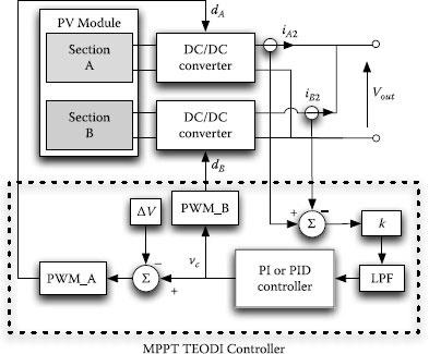
FIGURE 2.30
Block scheme of TEODI for parallel configuration of the power stages.

The duty cycles d_A and d_B of the two DC/DC converters are different because d_A = d_B − Δd, where Δd = ΔV/Vs, Vs is the peak amplitude of the sawtooth carrier waveforms of the two PWM modulators, and ΔV is a constant voltage offset that will be used to settle the TEODI performances. In particular, on the basis of the converter topology, such a parameter defines the voltage displacement (ΔV_pv) between the PV operating points of the two identical PV sections.

By assuming that the sign of the displacement voltage ΔV is chosen in order to obtain V_PV,A > V_PV,B, three conditions are possible for the operating points of the two PV sections.

Figure 2.31 shows the P-V curves of both PV sections, the square markers highlighting the operating points of PV section A and the circle markers putting into evidence the operating points of PV section B. In the case shown in Figure 2.31a, the PV power of section A is higher than that delivered by section B, thus corresponding to the condition i_A2 > i_B2 at the converter output. In the case shown in Figure 2.31b, the PV power delivered by section A is lower than that produced by section B, thus corresponding to the condition i_A2 < i_B2. The signal k· (i_A2 − i_B2) is at the input of the proportional-integral (PI) controller. The integral action forces the change of the duty cycles d_A and d_B, thus pushing the operating points of the PV sections in the direction that minimizes the difference of the output currents. The sign of the coefficient k must be properly selected in order to associate the right direction to the duty cycles for driving the operating points toward the MPP. Only when the system is in the condition shown in Figure 2.31c does the PV power of section A equal the power of section B, thus corresponding to i_A2 = i_B2. In such a case, the input of the PI controller is zero, and consequently the converters’ duty cycles remain at a constant value.

As for Δd, in equilibrium conditions, the smaller the value of Δd, the smaller the distance between the operating point of each of the PV modules and the MPP, and thus the higher the MPPT efficiency. In practice, because of the effect of tolerances of the physical components of the two sections and of small, nonetheless unavoidable, effects (due to temperature, humidity, and so on) making the two subsystems not perfectly equal, too small values of Δd could lead to the failure of the TEODI technique. The value of Δd affects both the MPPT efficiency in steady state environmental conditions and the speed of the whole tracking process under environmental dynamic conditions. Indeed, the higher the value of Δd, the higher the MPPT promptness. If Δd = 0, in the case of two perfectly equal sections, in all three cases shown in Figure 2.31 the operating point of PV section A collapses in the same position of PV section B. The speed would be equal to zero because the error at the input of the PI controller is always zero, and the system would not be able to perform the tracking process. Therefore Δd must settle on the basis of a reasonable compromise between the steady-state MPPT efficiency and required dynamic performances of the system. Considerations similar to those referred to the P&O technique, and discussed in the previous sections, do apply.

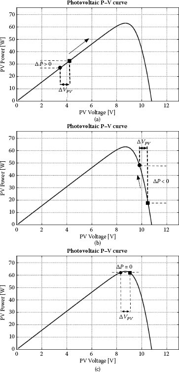
FIGURE 2.31
Power vs. voltage characteristic of photovoltaic modules A and B and the corresponding operating points.

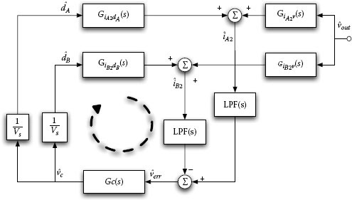
FIGURE 2.32
Equivalent block diagram of the TEODI architecture.

One of the main advantages of TEODI is in the simple design of the MPPT parameters because it consists of the right selection of the compensation network; such design can be performed directly in the Laplace’s domain by using the system transfer functions.

Given the TEODI architecture shown in Figure 2.30, the corresponding small-signal model can be obtained by averaging and linearizing the state equations of the whole system made of the converters, the load, and the PV sources.

In the equivalent block diagram shown in Figure 2.32 symbols with hats represent small-signal variations around the quiescent values of the corresponding quantities. The objective of the analysis in the Laplace domain is to identify conditions permitting the design of the transfer function W (s) = LPF(s)·G_c(s) leading to a stable closed-loop system, with an adequate phase margin and a sufficiently high crossover frequency.

By looking at the scheme in Figure 2.32, it results that the equilibrium point is reached when ${\widehat{i}}_{A2}={\widehat{i}}_{B2}$ and the system loop gain T_c(s) is given by

$T_c\left(s\right)=W\left(s\right)\cdot \left(G_{iA2dA}\left(s\right)-G_{iB2dB}\left(s\right)\right)$

(2.58)

The Bode diagram of the T_c(s) loop gain transfer function can be used to evaluate the system stability and dynamic performances of the TEODI algorithm. A particular aspect of the proposed architecture is in the fact that the T_c(s) transfer function has a double loop. The TEODI capability to reject the output voltage oscillations on the PV terminals can be evaluated by means of the $W_{v_{pv,A},v_o}\left(s\right)$ and $W_{v_{pv,B},v_o}\left(s\right)$ transfer functions:

$W_{vpv,A,v_o\left(s\right)}=\frac{{\widehat{v}}_{pv,A}}{{\widehat{v}}_{out}}=\frac{G_{vpv,A{v}_o\left(s\right)}}{1+T_c\left(s\right)}$

(2.59)

$W_{vpv,B,v_o\left(s\right)}=\frac{{\widehat{v}}_{pv,B}}{{\widehat{v}}_{out}}=\frac{G_{vpv,B{v}_o\left(s\right)}}{1+T_c\left(s\right)}$

(2.60)

where $G_{v_{pv,A}{v}_o}\left(s\right)$ and $G_{v_{pv,B}{v}_o}\left(s\right)$ are the output-to-input open-loop transfer functions of the converters used in the corresponding PV sections. Finally the effect of the output voltage oscillation on the TEODI control signal is given by

$W_{verr,vout\left(s\right)}=\frac{{\widehat{v}}_{err}}{{\widehat{v}}_{out}}=LPF\left(s\right)\cdot \frac{G_{iA2v\left(s\right)}-G_{iB2v\left(s\right)}}{1+T_c\left(s\right)}$

(2.61)

In the frequency range where the condition T_c(s) >> 1 holds, the system rejection capability is improved with respect to the open-loop system.

The reader can find further details and numerical examples of the TEODI approach in [36,37,38].

2.8    MPPT Efficiency

Up to few years ago no guidelines about the benchmarking of different MPPT techniques were available, but only some indication about the reasonable speed of variation of the irradiance to be used in testing an MPPT technique was given. For example, in [40], the slope 30 W/m²/s is considered a reference value. More recently, a standard for testing DC/AC inverters’ efficiency, the EN 50530, has been introduced, and a part of it is devoted to fix the conditions the MPPT algorithm must be subjected to for testing its performances. Steady-state and time-varying irradiation values and slopes are given, and some authors have published the results of their experimental analyses aimed at comparing the most famous MPPT approaches. For instance, in [41], the author assesses that the performances that can be obtained by the two most used algorithms, the P&O and the INC, are approximately the same. The fundamental role of the MPPT efficiency has not been recognized as the conversion efficiency is. In fact, many efforts are usually done by power electronics designers in order to increase the conversion efficiency of the power processing system. In addition to the classical peak efficiency value, the European efficiency (η_ev) has been proposed as a measure of the performances of the conversion system at different power levels, which means at different irradiation levels along the day. The European efficiency is defined in (2.62) in order to give a weight to the conversion efficiencies in the beginning of the day and approaching sunset, so that a power processing system having a flat and high-efficiency profile has a high η_EU.

${\text{η}}_{Eu}=0.03\cdot {\text{η}}_{5\%}+0.06\cdot {\text{η}}_{10\%}+0.13\cdot {\text{η}}_{20\%}+0.10\cdot {\text{η}}_{30\%}+0.48\cdot {\text{η}}_{50\%}+0.20\cdot {\text{η}}_{100\%}$

(2.62)

A similar formula has been also proposed by the Californian Energy Commission: The weights are different but the idea is the same.

${\text{η}}_{CEC}=0.00\cdot {\text{η}}_{5\%}+0.04\cdot {\text{η}}_{10\%}+\mathrm{0.0.05}\cdot {\text{η}}_{20\%}+0.12\cdot {\text{η}}_{30\%}+0.21\cdot {\text{η}}_{50\%}+0.53\cdot {\text{η}}_{75\%}+0.5\cdot {\text{η}}_{100\%}$

(2.63)

Nevertheless, the in-depth studies concerning the MPPT efficiency and the factors affecting its value are very few in literature, essentially because of the difficulty in understanding that the efficiency of the PV system is almost the product of the MPPT efficiency and the conversion efficiency.

The MPPT efficiency is defined as follows:

${\text{η}}_{MPPT}=\frac{{\displaystyle {\int }_{t1}^{t2}P\left(t\right)dt}}{{\displaystyle {\int }_{t1}^{t2}{P}_{MPP}\left(t\right)dt}}$

(2.64)

so that its value is unitary if the operating point remains in the MPP during the whole time interval going from t₁ to t₂. An approximation of the MPPT efficiency can be easily obtained by assuming that the P-V curve of the PV array behaves like a parabola across the MPP (see Figure 2.33). This analysis allows us to show what is the best steady-state condition that can be obtained by any perturbative MPPT approach. The first analysis is performed by supposing that there are operating points, with the one in the middle placed in the MPP and the side ones at the same power level, because of the parabolic approximation, on the ascending and descending sides of the P-V curve, respectively.

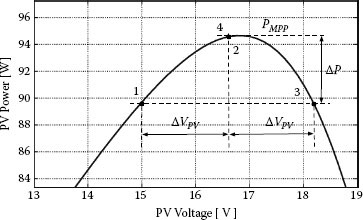
FIGURE 2.33
Three-point behavior in steady state.

If the MPPT controller leaves the system working in each one of these points for T_p seconds, then the waveform of the power looks as depicted in Figure 2.34.

The period of this waveform is 4·T_p, and due to the piecewise constant waveform of the PV power, it is easy to determine the numerator of (2.64), so that the MPPT efficiency is

${\text{η}}_{MPPT}=1-\frac{\text{Δ}P}{2\cdot P_{MPP}}$

(2.65)

where ΔP depends on the amplitude of the perturbation applied to implement the perturbative MPPT method and on the PV array parameters and operating conditions.

If the steady-state operation consists of four points, two on one side and two on the other side of the MPP, under the same assumption of a parabolic P-V curve with the vertex in the MPP, it results that

${\text{η}}_{MPPT}=\frac{<P\left(t\right){>}_{6\cdot T_p}}{P_{MPP}}=1-\frac{\text{Δ}{P}_1+\text{Δ}{P}_2}{2\cdot P_{MPP}}$

(2.66)

where the condition under analysis is shown in Figures 2.35 and 2.36.

Equations (2.65) and (2.66) reveal that the best condition in terms of MPPT efficiency is achieved when the steady state consists of three points, one in the MPP and two on its sides. The condition consisting of four points, and of course of more than four points, leads to a reduction of the MPPT efficiency and must be avoided as much as possible. In Section 2.4.2 the value of the power drops ΔP used in the expressions above has been calculated as a function of the amplitude of the perturbation signal used in the perturbative MPPT approach and of the PV array parameters.

FIGURE 2.34
Power waveform in steady state.

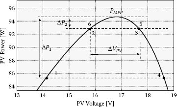
FIGURE 2.35
Four-point behavior in steady state.

FIGURE 2.36
Power waveform in four points in steady state.

References

1.  S.-K. Ji, D.-H. Jang, S.-K. Han, C.-W. Roh, and S.-S. Hong. Analog control algorithm for maximum power tracker employed in photovoltaic applications. In 2010 Conference Proceedings of IPEC, October 2010, pp. 99–103.

2.  J.H.R. Enslin, M.S. Wolf, D.B. Snyman, and W. Swiegers. Integrated photovoltaic maximum power point tracking converter. IEEE Transactions on Industrial Electronics, 44(6):769–773, 1997.

3.  W. Xiao, W.G. Dunford, P.R. Palmer, and A. Capel. Application of centered differentiation and steepest descent to maximum power point tracking. IEEE Transactions on Industrial Electronics, 54(5):2539–2549, 2007.

4.  M.A.S. Masoum, H. Dehbonei, and E.F. Fuchs. Theoretical and experimental analyses of photovoltaic systems with voltage and current-based maximum power-point tracking. IEEE Transactions on Energy Conversion, 17(4):514–522, 2002.

5.  C. Larbes, S.M. Aït Cheikh, T. Obeidi, and A. Zerguerras. Genetic algorithms optimized fuzzy logic control for the maximum power point tracking in photo-voltaic system. Renewable Energy, 34(10):2093–2100, 2009.

6.  C.-S. Chiu and Y.-L. Ouyang. Robust maximum power tracking control of uncertain photovoltaic systems: A unified t-s fuzzy model-based approach. IEEE Transactions on Control Systems Technology, 19(6):1516–1526, 2011.

7.  V. Salas, E. Olìas, A. Barrado, and A. Làzaro. Review of the maximum power point tracking algorithms for stand-alone photovoltaic systems. Solar Energy Materials and Solar Cells, 90:1555–1576, 2006.

8.  E. Koutroulis, K. Kalaitzakis, and N.C. Voulgaris. Development of a microcontroller-based, photovoltaic maximum power point tracking control system. IEEE Transactions on Power Electronics, 16(1):46–54, 2001.

9.  N. Femia, G. Petrone, G. Spagnuolo, and M. Vitelli. Optimization of perturb and observe maximum power point tracking method. IEEE Transactions on Power Electronics, 20(4):963–973, 2005.

10.  R.P. Venturini, V.V.R. Scarpa, G. Spiazzi, and S. Buso. Analysis of limit cycle oscillations in maximum power point tracking algorithms. In IEEE Power Electronics Specialists Conference 2008 (PESC 2008), June 2008, pp. 378–384.

11.  S. Liu and R.A. Dougal. Dynamic multiphysics model for solar array. IEEE Transactions on Energy Conversion, 17(2):285–294, 2002.

12.  R.W. Erikson and D. Maksimovic. Fundamentals of power electronics. 2nd ed. Kluwer Academic Publishers, Norwell, MA.

13.  F.L. Luo and H. Ye. Small signal analysis of energy factor and mathematical modeling for power dc-dc converters. IEEE Transactions on Power Electronics, 22(1):69–79, 2007.

14.  K.H. Hussein, I. Muta, T. Hoshino, and M. Osakada. Maximum photovoltaic power tracking: An algorithm for rapidly changing atmospheric conditions. IEE Proceedings on Generation, Transmission and Distribution, 142(1):59–64, 1995.

15.  R. Bründlinger, N. Henze, H. Häberlin, B. Burger, A. Bergmann, and F. Baumgartner. prEN50530—The new European standard for performance characterisation of pv inverters. In 24th European Photovoltaic Solar Energy Conference, Hamburg, Germany, September 2009, vol. 1, pp. 3105–3109.

16.  W. Xiao and W.G. Dunford. A modified adaptive hill climbing MPPT method for photovoltaic power systems. In 2004 IEEE 35th Annual Power Electronics Specialists Conference (PESC 04), June 2004. vol. 3, pp. 1957–1963.

17.  A. Pandey, N. Dasgupta, and A.K. Mukerjee. Design issues in implementing MPPT for improved tracking and dynamic performance. In 32nd Annual Conference on IEEE Industrial Electronics, IECON 2006, November 2006, pp. 4387–4391.

18.  N. Fermia, D. Granozio, G. Petrone, and M. Vitelli. Predictive adaptive MPPT perturb and observe method. IEEE Transactions on Aerospace and Electronic Systems, 43(3):934–950, 2007.

19.  Y.-T. Hsiao and C.-H. Chen. Maximum power tracking for photovoltaic power system. In 37th IAS Annual Meeting of Industry Applications Conference, 2002, vol. 2, pp. 1035–1040.

20.  D.P. Hohm and M.E. Ropp. Comparative study of maximum power point tracking algorithms. Progress in Photovoltaics: Research and Applications, 11(1):47–62, 2003.

21.  F.-S. Pai, R.-M. Chao, S.H. Ko, and T.-S. Lee. Performance evaluation of parabolic prediction to maximum power point tracking for PV array. IEEE Transactions on Sustainable Energy, 2(1):60–68, 2011.

22.  K. Ishaque, Z. Salam, M. Amjad, and S. Mekhilef. An improved particle swarm optimization (PSO)-based MPPT for PV with reduced steady state oscillation. IEEE Transactions on Power Electronics, PP(99):1, 2012.

23.  M. Miyatake, M. Veerachary, F. Toriumi, N. Fujii, and H. Ko. Maximum power point tracking of multiple photovoltaic arrays: A PSO approach. IEEE Transactions on Aerospace and Electronic Systems, 47(1):367–380, 2011.

24.  G. Petrone, G. Spagnuolo, and M. Vitelli. A multivariable perturb-and-observe maximum power point tracking technique applied to a single-stage photovoltaic inverter. IEEE Transactions on Industrial Electronics, 58(1):76–84, 2011.

25.  A.M. Bazzi and P.T. Krein. Concerning “Maximum power point tracking for photovoltaic optimization using ripple-based extremum seeking control.” IEEE Transactions on Power Electronics, 26(6):1611–1612, 2011.

26.  A.I. Bratcu, I. Munteanu, S. Bacha, D. Picault, and B. Raison. Cascaded DC-DC converter photovoltaic systems: Power optimization issues. IEEE Transactions on Industrial Electronics, 58(2):403–411, 2011.

27.  S.L. Brunton, C.W. Rowley, S.R. Kulkarni, and C. Clarkson. Maximum power point tracking for photovoltaic optimization using ripple-based extremum seeking control. IEEE Transactions on Power Electronics, 25(10):2531–2540, 2010.

28.  D. Casadei, G. Grandi, and C. Rossi. Single-phase single-stage photovoltaic generation system based on a ripple correlation control maximum power point tracking. IEEE Transactions on Energy Conversion, 21(2):562–568, 2006.

29.  T. Esram, J.W. Kimball, P.T. Krein, P.L. Chapman, and P. Midya. Dynamic maximum power point tracking of photovoltaic arrays using ripple correlation control. IEEE Transactions on Power Electronics, 21(5):1282–1291, 2006.

30.  J.W. Kimball and P.T. Krein. Discrete-time ripple correlation control for maximum power point tracking. IEEE Transactions on Power Electronics, 23(5):2353–2362, 2008.

31.  K.H. Hussein, I. Muta, T. Hoshino, and M. Osakada. Maximum photovoltaic power tracking: An algorithm for rapidly changing atmospheric conditions. IEE Proceedings of Generation, Transmission and Distribution, 142(1):59–64, 1995.

32.  F. Liu, S. Duan, F. Liu, B. Liu, and Y. Kang. A variable step size INC MPPT method for PV systems. IEEE Transactions on Industrial Electronics, 55(7):2622–2628, 2008.

33.  Q. Mei, M. Shan, L. Liu, and J.M. Guerrero. A novel improved variable step-size incremental-resistance MPPT method for PV systems. IEEE Transactions on Industrial Electronics, 58(6):2427–2434, 2011.

34.  D. Shmilovitz. On the control of photovoltaic maximum power point tracker via output parameters. IEE Proceedings of Electric Power Applications, 152(2):239–248, 2005.

35.  L. Egiziano, N. Femia, G. Lisi, G. Petrone, G. Spagnuolo, and M. Vitelli. Design and optimization of a maximum power point tracking controller for a PV battery charger. In IEEE International Symposium on Industrial Electronics, 2007 (ISIE 2007), June 2007, pp. 2426–2431.

36.  N. Femia, G. Petrone, G. Spagnuolo, and M. Vitelli. A new analog MPPT technique: TEODI. Progress in Photovoltaics: Research and Applications, 18(1):28–41, 2010.

37.  G. Petrone, G. Spagnuolo, and M. Vitelli. TEODI: A new technique for distributed maximum power point tracking PV applications. In 2010 IEEE International Conference on Industrial Technology (ICIT), March 2010, pp. 982–987.

38.  G. Petrone, G. Spagnuolo, and M. Vitelli. TEODI: PV MPPT based on the equalization of the output operating points in correspondence of the forced displacement of the input operating points. In 2010 IEEE International Symposium on Industrial Electronics (ISIE), July 2010, pp. 3463–3468.

39.  N. Femia, G. Lisi, G. Petrone, G. Spagnuolo, and M. Vitelli. Distributed maximum power point tracking of photovoltaic arrays: Novel approach and system analysis. IEEE Transactions on Industrial Electronics, 55(7):2610–2621, 2008.

40.  B. Bletterie, R. Bruendlinger, and S. Spielauer. Quantifying dynamic MPPT performance under realistic conditions first test results—The way forward. In Proceedings of 21st European Photovoltaic Solar Energy Conference and Exhibition, 2006, pp. 2347–2351.

41.  T. Andrejasic, M. Jankovec, and M. Topic. Comparison of direct maximum power point tracking algorithms using en 50530 dynamic test procedure. IET Renewable Power Generation, 5(4):281–286, 2011.

*  The reader can find additional information on the switching ripple attenuation in Section 3.4.