1

PV Modeling

1.1    From the Photovoltaic Cell to the Field

Photovoltaic (PV) generators are made of a number of PV cells connected in series and in parallel. The type of connection depends on the voltage and current levels at which it is desired that the power processing system dedicated to the PV generator works. The right choice of the values of such electrical variables is of fundamental importance in determining the efficiency of the switching converters that condition the power produced by the PV generator in order to feed the AC mains or recharge a battery. Unfortunately, in usual applications the voltage and current levels of the PV generator cannot be referred to a single PV cell. In fact, cells are arranged into PV panels, which contain some tens of them connected in series. The choice of connecting the cells in series comes from the fact that their operating voltage is few hundreds of millivolts, while the current they generate at high irradiation levels is of some amperes. As a consequence, the cells series connection leads to PV panels working at few tens of volts and some amperes.

In PV power plants, panels are connected in series to form strings in order to reach a voltage level that meets the input requirements of the power processing system. The desired power level of the PV plant is reached by connecting a number of strings, each one composed of the same number of panels, in parallel, thus leading to an increase of the current level of the PV field.

The nominal current vs. voltage (I-V) characteristic of the whole PV field is obtained by stretching that of the single cell, namely by multiplying the voltage values by the number of cells in series into each panel and then by the number of panels of each string, and by multiplying the cell current values by the number of strings of panels connected in parallel.

Such a voltage and current scaling up holds only under the hypotheses that all the cells are exactly equal and that they work in exactly the same operating conditions, especially in terms of irradiance and temperature. Unfortunately such conditions do not occur in practice because of manufacturing tolerances and aging, so that physical parameters of the cells are different, and because of shadowing, of the different orientation of the cells with respect to the sun rays, due to leaves, bird droppings, and so on.

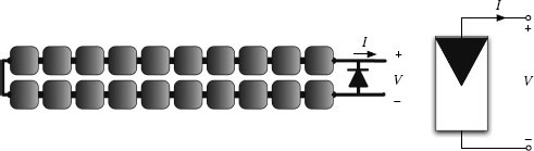
FIGURE 1.1
PV module made of some cells and the bypass diode.

Nonuniform operating conditions are usually referred to as mismatching, and they can lead to significant drops in the energy produced by the PV field. This mechanism will be explained in much more detail in this chapter, but a simple example can be instructive now. If, due to an accident, one cell is broken or simply disconnected from the contiguous ones, then the current of all the cells in series in the string is interrupted and the power contribution of the whole string is missed.

To reduce the effect of such events, PV panel manufacturers connect a bypass diode in parallel to short strings of series connected cells, usually two or three depending on the power rating forming the PV panels. In this way, a PV panel is made of two or three PV modules, structured as shown in Figure 1.1. In the sequel, if the modules the PV panel is made of join the same operating conditions and are perfectly equal, the terms module and panel will be assumed as synonyms.

The diodes are physically mounted into a junction box on the rear side of the panel and are normally inactive. Each of them fires as soon as the group of cells it is dedicated to generates a current lower than the one of the other subpanels in the string, so that it bypasses the exceeding current. Such a mechanism will be described in this chapter, showing the effects the bypass diode may have on the electrical characteristics of the whole string and field, as well as on the cells, owing to the bypassed group. The electrical structure of the PV panel just described changes the level of granularity at which the PV generator is considered in this book. Indeed, the PV generator becomes a parallel connection of strings, each one made of a series connection of PV modules, as shown in Figure 1.2.

In order to understand the way in which current and voltages are shared among the PV modules, especially in mismatched conditions, a model of the generator is required. The model is as very useful, as its level of complexity allows embedding it into circuits and systems simulation and computing programs of general use, like PSIM^®, SPICE^®, and MATLAB^®/Simulink^®.*

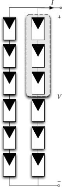
FIGURE 1.2
From module to field.

This chapter is devoted to the description of the PV generator operation, in both uniform and mismatched conditions, by means of nonlinear models. The models and the conclusions they lead to will be useful for the full comprehension of the concepts described in the following chapters of the book.

1.2    The Electrical Characteristic of a PV Module

The electrical characteristics of a PV panel working in uniform conditions are plotted in Figures 1.3 to 1.6 in normalized units. T_max and G_max can be assumed as the values used for testing the panel in standard conditions. Such curves are a qualitative example because, as will be much more clear in the sequel, their characteristics depend on the type of cells, materials, and technical solutions adopted for manufacturing the panel.

The plots put into evidence the presence of a maximum power point (MPP). Figures 1.5 and 1.6 show that the curves exhibit three particular points:

•  The short-circuit (SC) condition, characterized by a zero voltage at the PV module terminals and by a short-circuit current I_SC

FIGURE 1.3
Current vs. voltage characteristic of a PV panel: effect of temperature T.

•  The open-circuit (OC) condition, characterized by a zero current in the PV panel terminals and by an open-circuit voltage V_OC

•  The MPP, at which the current value is I_MPP, the voltage value is V_MPP, and the power P_MPP = V_MPP · I_MPP is the maximum the PV panel is able to deliver in the temporary operating conditions

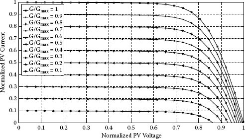
FIGURE 1.4
Current vs. voltage characteristic of a PV panel: effect of irradiation G.

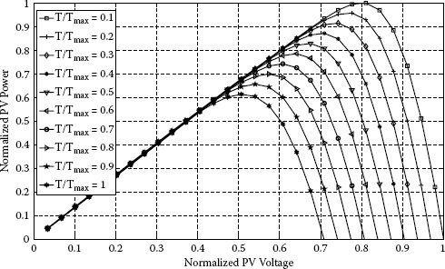
FIGURE 1.5
Power vs. voltage characteristic of a PV panel: effect of temperature T.

Figures 1.3 to 1.6 put into evidence the strong dependence of the panel performances on the temperature and the irradiance level. The temperature has a significant effect on the open-circuit voltage value, as shown in Figures 1.3 and 1.5. On the contrary, the temperature has a negligible effect on the short-circuit current value. The cell temperature, here indicated as T, is calculated from the ambient temperature T_a by using the nominal operating cell temperature (NOCT)*:

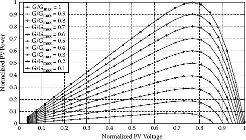
FIGURE 1.6
Power vs. voltage characteristic of a PV panel: effect of irradiation G.

$T=T_a+\frac{NOCT-20}{800}\cdot G$

(1.1)

It is worth noting that the temperature usually changes quite slowly, so that the temperature value is often considered a constant with respect to the variation the irradiation level can be subjected to during the day. This simplifying assumption will be also adopted in this book.

The irradiance variation has dual effects on the electrical characteristics with respect to the temperature. The PV module open-circuit voltage is almost independent of the irradiation: in literature it is stated that such a dependence is logarithmic. On the contrary, the short-circuit current is linearly dependent on the irradiance.

Electrical characteristics of PV modules are given by manufacturers in specific operating conditions, which are worldwide defined as standard test conditions (STC). Such conditions are defined by the cell temperature T_STC = 25°C, irradiation level G_STC = 1000 W/m², and the air mass value AM = 1.5. The latter gives a measure of the effect of the air mass between a surface and the sun on the spectral distribution and intensity of sunlight. In fact, the path length of the solar radiation through the atmosphere affects the light deviation and absorption [1, 2].

The irradiance variation is considered the main perturbing factor to be faced, because of its unpredictability: its effects will be widely discussed in this book. The irradiation rate of change is another unpredictable variable that must be taken into account: According to [3], the usual irradiance slope is $\dot{G}=30W/m^2/s$. Such value is referred to classical stationary PV applications; more recent applications of PV systems, e.g. sustainable mobility, require performing the analysis with much more critical values of $\dot{G}$. For this reason, in this book higher values will also be considered.

The best way to analyze the behavior of the PV generator in a simulation environment is to adopt an equivalent circuit model and relevant equations describing it. In the sequel, such models are introduced and a special emphasis is devoted to the identification of the parameters either on the basis of the data obtained from experimental measurements or starting from data sheet information.

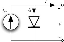
FIGURE 1.7
Ideal equivalent circuit of a PV generator.

1.3    The Double-Diode and Single-Diode Models

Looking at the figures shown in the previous section reveals that the I-V curve of a PV generator is obtained by subtracting a diode current, which is nonlinearly dependent on its voltage, from a constant current value. As a consequence, the ideal equivalent circuit shown in Figure 1.7 is made of a current generator in parallel with a diode.

The diode takes into account the physical effects taking place at the silicon p-n junction of the cell. The current generator represents the photo-induced current, which is dependent on the characteristics of the semiconductor material used for the cell, and especially, it is linearly dependent on the cell area, irradiation level, and temperature. Equation (1.2) gives the dependency on the two latter exogenous variables:

$I_{ph}=I_{ph,STC}\cdot \frac{G}{G_{STC}}\cdot \left[1+{\text{α}}_I\cdot \left(T-T_{STC}\right)\right]$

(1.2)

where α_I is the temperature coefficient of the current, defined in STC as follows:

${\text{α}}_I={\frac{dI}{dT}|}_{STC}$

(1.3)

As a consequence, the I-V characteristic takes the form shown in (1.4).

$I=I_{ph}-I_{sat}\cdot \left(e^{\frac{V}{{\text{η}V}_t}}-1\right)$

(1.4)

where, as usual, V_t is the thermal voltage (1.5):

$V_t=\frac{k\cdot T}{q}$

(1.5)

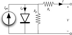
FIGURE 1.8
Single-diode model accounting for ohmic losses.

k = 1.3806503·10−23 J/K is the Boltzmann constant, q = 1.60217646 · 10−19 C is the electron charge, and η is the ideality factor. The saturation current is expressed as follows:

$I_{sat}=C\cdot T^3\cdot e^{\left(-\frac{E_{gap}}{kT}\right)}$

(1.6)

where E_gap is the band gap of the semiconductor material* and C is the temperature coefficient [2].

Such a model does not take into account either the loss mechanisms taking place in the cell due to the metallic ribbon ensuring the current continuity between each cell and the two cells before and after it in the sequence or the diffusion and recombination characteristics of the charge carriers in the semiconductor. Such losses are introduced in the model by adding a series R_s and a parallel R_p resistance in order to take into account internal cell resistances and contact resistances, as well as the effect of leakage currents, respectively. As a consequence, the model becomes the one shown in Figure 1.8.

The series resistance R_s mainly affects the slope of the I-V curves in Figures 1.3 and 1.4 at high voltage levels, namely, approaching the open-circuit voltage: the worse the cell quality, the lower the curve slope, because of a high voltage drop across the series resistance. As a consequence, the approximated definition (1.7) can be adopted:

$R_s\approx -{\frac{dV}{dI}|}_{V=V_{OC}}$

(1.7)

On the other hand, R_p affects the curve slope at current levels close to the short-circuit one: the lower the R_p value, the higher the current drawn by the parallel resistance, which is subtracted from the net output current, witnessed by a smaller slope of the curve at low voltage values, where it is

$R_p\approx -{\frac{dV}{dI}|}_{I=I_{SC}}$

(1.8)

The values of these two resistances have an immediate effect on the cell energy productivity expressed through the index called fill factor, which is defined as the ratio between the product of the voltage and current values at the MPP and the product of the short-circuit current and open-circuit voltage values:

$FF=\frac{V_{MPP}\cdot I_{MPP}}{V_{OC}\cdot I_{SC}}$

(1.9)

In order to account for the ohmic losses, Equation (1.4) must be modified. According to Kirchhoff’s laws, Equation (1.10) is obtained.

$I=I_{ph}-I_{sat}\cdot \left(e^{\frac{V+I\cdot R_s}{{\text{η}V}_t}}-1\right)-\frac{V+I\cdot R_s}{R_p}$

(1.10)

It is worth noting that both (1.4) and (1.10) are nonlinear, but the latter is also in implicit form, because neither the current nor the voltage can be explicitly expressed as functions of the other electrical variable. As will be pointed out in Section 1.6, this represents a strong limitation for many theoretical and numerical analyses.

According to the Shockley theory, the equivalent circuit shown in Figure 1.8 describes diffusion and recombination characteristics of the charge carriers in the semiconductor, but it neglects the recombination in the space-charge zone. If such effect must to be taken into account, a two-diode model must be used.

The consequent I-V characteristic, expressed by Equation (1.11) and describing the equivalent circuit shown in Figure 1.9, is more involved:

$I=I_{ph}-I_{sat}\cdot \left(e^{\frac{V+I\cdot R_s}{{\text{η}V}_t}}-1\right)-I_{sat,2}\cdot \left(e^{\frac{V+I\cdot R_s}{{\text{η}}_2{V}_t}}-1\right)-\frac{V+I\cdot R_s}{R_p}$

(1.11)

where the second saturation current shows the following nonlinear dependence on temperature:

$I_{sat,2}=C_2\cdot T^{\frac{5}{2}}\cdot e^{\left(-\frac{E_{gap}}{2kT}\right)}$

(1.12)

In this book, the single-diode model shown in Figure 1.8 and described by the implicit equation (1.10) is used. Such a model holds for a single PV crystalline cell, and it can be scaled up suitably in order to also be used for a PV module, panel, string, or for the whole PV field.

Under the assumption that all the cells are equal and that they work in the same operating conditions, all the voltages will be multiplied by n_s, if this is the number of the series connected cells, and all the currents will be multiplied by n_p, if this is the number of parallel connected strings. Consequently, the series resistance R_s and the parallel resistance R_p increase by a factor n_s and are divided by a factor n_p. In symbols:

$I_{ph,field}=n_p\cdot I_{ph,cell}$

(1.13)

$I_{sat,field}=n_p\cdot I_{sat,cell}$

(1.14)

$V_{t,field}=n_s\cdot V_{t,cell}$

(1.15)

$R_{s,field}=\frac{n_s}{n_p}\cdot R_{s,cell}$

(1.16)

$R_{p,field}=\frac{n_s}{n_p}\cdot R_{p,cell}$

(1.17)

It is worth noting that according to the active sign convention chosen for the current and voltage in Figure 1.8, the first quadrant of the plots shown in Figures 1.3 and 1.4 refers to an operating condition in which the PV system generates electrical power. Nevertheless, as will be demonstrated in Section 1.6, in some conditions the PV generator can be polarized with a reverse voltage, which is negative with respect to the reference used in Figure 1.8. In this case, if the PV system is illuminated, the current keeps its direction; thus it is positive with respect to the reference used in Figure 1.8, and the system absorbs, rather than generates, electrical power. In this case, the operating point moves in the second quadrant of the Cartesian plot shown in Figures 1.3 and 1.4, and a suitable model of the physical effects taking place in such conditions is needed.

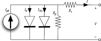
FIGURE 1.9
Two-diode equivalent circuit for a solar cell.

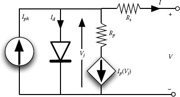
FIGURE 1.10
Bishop equivalent circuit for a counterpolarized solar cell.

According to [4], the shunt branch in Figure 1.8 must include a voltage-controlled current generator, so that the equivalent circuit becomes the one shown in Figure 1.10.

In this way, the current through the shunting branch is expressed as

$I_p=\frac{V_j}{R_p}\cdot \left[1+\text{α}\cdot {\left(1-\frac{V+I\cdot R_s}{V_{br}}\right)}^{-m}\right]$

(1.18)

where V_br is the junction breakdown voltage, α is the fraction of the ohmic current involved in avalanche breakdown, and m is the avalanche breakdown exponent. In some conditions, which will be discussed in Section 1.6, the voltage can assume large negative values, up to some tens of volts: Under a reverse voltage condition the cell can even dissipate a significant amount of electrical power, with a consequent increment in temperature and occurrence of hot spots. This may lead to an irreversible damaging of the cell, with a consequent interruption of the current flux into the whole string it belongs to. It is commonly believed that the bypass diode helps in reducing the probability that the reverse polarization of a cell determines hot spots and power losses, simply because it limits the reverse voltage to its direct polarization voltage, which is usually less than 1 V. This would be true if a bypass diode was used for each PV cell; however, due to the high number of diodes that such a solution would require for a PV panel realization, in practice a bypass diode is dedicated to a string of few tens of cells forming a PV module. In this case, the total reverse voltage of the cells in the PV module is limited by the forward voltage of the bypass diode, so that they are protected from hot spot occurrence, provided that they work in the same operating conditions. A different, and also more involved, study is required whenever mismatched conditions affect the cells of the PV module.

As a result of the discussion above, in Sections 1.4 and 1.6 the model in Equation (1.10) and the equivalent circuit in Figure 1.8 will be assumed to represent the string of PV cells into a PV module or panel, a string or the whole field, provided that the voltage, current, and resistance values are suitably scaled. Until no bypass diode conducts, the PV characteristic of a PV panel is obtained by scaling up that of a single module, so that the words module and panel have the same meaning.

1.4    From Data Sheet Values to Model Parameters

The circuit shown in Figure 1.8 and the corresponding equation (1.10) give the desired compromise between complexity and accuracy. The next task is the tuning of the model parameters to the PV module of interest. Two approaches are proposed in literature to solve this problem. The first is based on the best fitting of the I-V or P-V curves obtained by means of the model with the experimental measurement data obtained from the PV module testing. The data resulting from the experimental measurements correspond to points acquired at different voltage/current levels and for different irradiation/temperature values. When such data are available, some approaches presented in literature can be applied: For example, the mean square error fitting approach might be an option.

The most puzzling problem is the I-V and P-V curves reconstruction on the unique basis of the data available on the PV module data sheet. The difficulty arises from the fact that only the following information in STC is given therein:

•  Operation in open-circuit conditions: V_OC,STC

•  Open-circuit voltage/temperature coefficient: ${\alpha }_v={\frac{d{V}_{OC}}{dT}|}_{STC}$

•  Operation in short-circuit conditions: I_SC,STC

•  Short-circuit current/temperature coefficient: ${\alpha }_i={\frac{d{I}_{SC}}{dT}|}_{STC}$

•  Operation at the maximum power point: I_MPP,STC and V_MPP,STC

The availability of the set of the parameters listed above allows determining the values of five unknowns. If the single-diode model (1.10) is adopted, the values taken from the data sheet find their counterparts in the unknowns {I_ph, I_sat, η, R_s, R_p}.

1.4.1    Parameters Identification Assuming R_p → ∞

The problem is afforded in literature by using two approaches: A simplified one considers the value of the parallel resistance R_p so high that it can be neglected. In this case, the equation whose parameters need to be identified is (1.19).

$I=I_{ph}-I_{sat}\cdot \left[e^{\frac{\left(V+I\cdot R_s\right)}{{\text{η}V}_t}}-1\right]$

(1.19)

In [2], the procedure for parameters identification is divided into steps. The data sheet voltage values are preliminarily divided by the number n_s of series connected cells forming the PV panel. Then the photo-induced current is calculated straightforwardly, because it is significantly higher than the diode current, so that it is assumed to be equal to the short-circuit current in STC:

$I_{ph,STC}=I_{SC,STC}$

(1.20)

The second step starts by applying (1.19) in the open-circuit condition:

$0=I_{ph,STC}-I_{sat,STC}\cdot \left(e^{\frac{V_{OC,STC}/n_s}{{\text{η}V}_{t,STC}}}-1\right)\approx I_{ph,STC}-I_{sat,STC}\cdot e^{\frac{V_{OC,STC}/n_s}{{\text{η}V}_{t,STC}}}$

(1.21)

where the second equivalence has been obtained by neglecting the unitary term with respect to the exponential one. Consequently, it is

$V_{OC,STC}\approx -\text{η}\cdot n_s\cdot V_{t,STC}\cdot \ln \left(\frac{I_{sat,STC}}{I_{ph,STC}}\right)$

(1.22)

The open-circuit voltage temperature coefficient can be calculated as follows:

${\text{α}}_v=\frac{d{V}_{OC,STC}}{dT}=\frac{d}{dT}\left[n_s\cdot \text{η}\cdot V_{t,STC}\cdot \ln I_{ph,STC}-n_s\cdot \text{η}\cdot V_{t,STC}\cdot \ln I_{sat,STC}\right]$

(1.23)

Accounting for the temperature dependence of the thermal voltage (1.5) yields

${\text{α}}_v=\frac{n_s\cdot \text{η}\cdot V_{t,STC}}{T_{STC}}\cdot \ln \left(\frac{I_{ph,STC}}{I_{sat,STC}}\right)+n_s\cdot \text{η}\cdot V_{t,STC}\cdot \left[\frac{1}{I_{ph,STC}}\cdot \frac{d{I}_{ph,STC}}{dT}-\frac{1}{I_{sat,STC}}\cdot \frac{d{I}_{sat,STC}}{dT}\right]$

(1.24)

The second term in the parentheses can be calculated by means of (1.6)

$\frac{1}{I_{sat,STC}}\cdot \frac{d{I}_{sat,STC}}{T_{STC}}=\frac{3}{T_{STC}}+\frac{E_{gap}}{k\cdot T_{STC}^2}$

(1.25)

while the first term is related to the current temperature coefficient α_i, so that

${\text{α}}_v=\frac{n_s\cdot \text{η}\cdot V_{t,STC}}{T_{STC}}\cdot \ln \left(\frac{I_{ph,STC}}{I_{sat,STC}}\right)+n_s\cdot \text{η}\cdot V_{t,STC}\cdot \left(\frac{{\text{α}}_i}{I_{ph,STC}}-\frac{3}{T_{STC}}-\frac{E_{gap}}{k\cdot T_{STC}^2}\right)$

(1.26)

From (1.22) it is

${\text{α}}_v=\frac{V_{OC,STC}}{T_{STC}}+n_s\cdot \text{η}\cdot V_{t,STC}\cdot \left(\frac{{\text{α}}_i}{I_{ph,STC}}-\frac{3}{T_{STC}}-\frac{E_{gap}}{k\cdot T_{STC}^2}\right)$

(1.27)

thus the diode ideality factor is calculated by means of (1.28):

$\text{η}=\frac{{\text{α}}_v-\frac{V_{OC,STC}}{T_{STC}}}{n_s\cdot V_{t,STC}\cdot \left(\frac{{\text{α}}_i}{I_{ph,STC}}-\frac{3}{T_{STC}}-\frac{E_{gap}}{k\cdot T_{STC}^2}\right)}$

(1.28)

In order to calculate I_sat, the open-circuit conditions can be used as well, so that from (1.21) it is

$I_{sat,STC}\approx I_{ph,STC}\cdot e^{-\frac{V_{OC,STC}}{\text{η}\cdot n_s\cdot V_{t,STC}}}$

(1.29)

so that the temperature coefficient C in (1.6) can be evaluated and I_sat can be calculated at the desired value of temperature T.

$C=\frac{I_{sat,STC}}{T_{STC}3.e^{-\frac{E_{gap}}{k\cdot T_{STC}}}}$

(1.30)

The series resistance can be determined by using the MPP data:

$I_{MPP,STC}=I_{ph,STC}-I_{sat,STC}\cdot \left[e^{\frac{V_{MPP,STC}+I_{MPP,STC}\cdot R_s}{\text{η}{n}_s\cdot V_{t,STC}}}-1\right]\approx I_{ph,STC}-I_{sat,STC}\cdot e^{{}^{\frac{V_{MPP,STC}+I_{MPP,STC}\cdot R_s}{\text{η}{n}_s\cdot V_{t,STC}}}}$

(1.31)

Substituting (1.29) into (1.31) yields

$I_{MPP,STC}=I_{ph,STC}-I_{ph,STC}\cdot \left[e^{\frac{\left(-V_{OC,STC}+V_{MPP,STC}+R_s\cdot I_{MPP,STC}\right)}{\text{η}{n}_s\cdot V_{t,STC}}}\right]$

(1.32)

thus the series resistance can be calculated by means of (1.33).

$R_s=\frac{n_s\cdot \text{η}\cdot V_{t,STC}\cdot \ln \left(1-\frac{I_{MPP,STC}}{I_{ph,STC}}\right)+V_{OC,STC}-V_{MPP,STC}}{I_{MPP,STC}}$

(1.33)

Equations (1.20), (1.30), (1.28), and (1.33) allow calculation of the four values of the unknown parameters in (1.19) starting from the data {V_oc, I_sc, α_i, α_v, V_MPP, I_MPP} in the STC available in the PV panel data sheets provided by the manufacturers.

As shown in Section 1.4.2, if the R_p value is accounted for, the procedure becomes much more involved and not straightforward, as it requires the solution of a nonlinear system of equations. An approximate solution might be obtained if some simplification of small terms with respect to larger ones is done. This result will be shown in Section 1.4.3.

1.4.2    Parameters Identification Including R_p

The approach proposed in the previous section can be extended by accounting for the presence of the parallel resistance. Equation (1.10), applied at the MPP, can be used to express the parallel resistance as a function of the series one:

$R_p=\frac{V_{MPP,STC}+I_{MPP,STC}\cdot R_s}{I_{ph}-I_{MPP,STC}-I_{sat,STC}\cdot \left(e^{\frac{V_{MPP,STC}+I_{MPP,STC}\cdot R_s}{\text{η}{V}_{t,STC}}}-1\right)}$

(1.34)

where the module thermal voltage V_t is related to the thermal voltage of the single cell V_T multiplied by the number of cell in series: V_t = n_sV_T.

The second equation, which completes the nonlinear system allowing calculation of both R_s and R_p, is obtained by observing that at the MPP the following condition holds:

${\frac{\partial \left(V\cdot I\right)}{\partial V}|}_{MPP,STC}=0\to I_{MPP,STC}+V_{MPP,STC}\cdot {\frac{\partial I}{\partial V}|}_{MPP,STC}=0$

(1.35)

thus using (1.10) yields:

${\frac{\partial I}{\partial V}|}_{MPP,STC}=-\frac{\frac{1}{R_p}+\frac{I_{sat,STC}}{\text{η}\cdot V_{t,STC}}\cdot e^{\frac{V_{MPP,STC}+I_{MPP,STC}\cdot R_s}{\text{η}{V}_{t,STC}}}}{1+\frac{R_s}{R_p}+\frac{Rs\cdot I_{sat,STC}}{\text{η}\cdot V_{t,STC}}\cdot e^{\frac{V_{MPP,STC}+I_{MPP,STC}\cdot R_s}{\text{η}{V}_{t,STC}}}}$

(1.36)

The second equation is obtained by substituting the above result in (1.35), so that

$I_{MPP,STC}-V_{MPP,STC}\cdot \frac{\frac{1}{R_p}+\frac{I_{sat,STC}}{\text{η}\cdot V_{t,STC}}\cdot e^{\frac{V_{MPP,STC}+I_{MPP,STC}\cdot R_s}{\text{η}{V}_{t,STC}}}}{1+\frac{R_s}{R_p}+\frac{Rs\cdot I_{sat,STC}}{\text{η}\cdot V_{t,STC}}\cdot e^{\frac{V_{MPP,STC}+I_{MPP,STC}\cdot R_s}{\text{η}{V}_{t,STC}}}}=0$

(1.37)

The joint solution of the nonlinear equations (1.34) and (1.37) provides the values or the series and parallel resistances.

1.4.3    Parameters Identification Including R_p: Explicit Solution

Based on the change of variable

$x=\frac{V_{MPP,STC}+R_s\cdot I_{MPP,STC}}{\text{η}{V}_{t,STC}}$

(1.38)

the series and parallel resistances can be written, using (1.38) and (1.34), as follows:

$R_s=\frac{x\text{η}{V}_{t,STC}-V_{MPP,STC}}{I_{MPP,STC}}\text{;}{R}_p=\frac{x\text{η}{V}_{t,STC}}{I_{ph}-I_{MPP,STC}-I_{sat,STC}\cdot \left(e^x-1\right)}$

(1.39)

After substituting such expressions in (1.37), the term ηV_τ, _STCx² appears. A few algebra steps, neglecting the small quantity term $R_s^2$, lead to

$\text{η}{V}_{t,STC}{x}^2\approx -\frac{V_{MPP,STC}^2}{\text{η}{V}_{t,STC}}+2\cdot V_{MPP,STC}\cdot x$

(1.40)

Consequently, it results that solving (1.37) means solving (1.41) with respect to x:

$2V_{MPP,STC}\cdot \left(I_{MPP,STC}-I_{ph}-I_{sat,STC}\right)+\left(I_{ph}+I_{sat,STC}\right)\text{η}{V}_{t,STC}\cdot x+I_{sat,STC}\cdot e^x\left[-\text{η}{V}_{t,STC}x+V_{MPP,STC}\cdot \left(2-\frac{V_{MPP,STC}}{\text{η}{V}_{t,STC}}\right)\right]=0$

(1.41)

The first two terms in (1.41) can be simplified, by accounting for (1.39), as follows:

$\begin{array}{l}2V_{MPP,STC}\cdot \left(I_{MPP,STC}-I_{ph}-I_{sat,STC}\right)+\left(I_{ph}+I_{sat,STC}\right)\text{η}{V}_{t,STC}x\\ =V_{MPP,STC}\cdot \left(2\cdot I_{MPP,STC}+I_{ph}+I_{sat,STC}\right)+\left(I_{ph}+I_{sat,STC}\right)\cdot \left(R_s\cdot I_{MPP,STC}-2\cdot V_{MPP,STC}\right)\\ \approx V_{MPP,STC}\cdot \left(2I_{MPP,STC}+I_{ph}+I_{sat,STC}\right)-2\cdot \left(I_{ph}+I_{sat,STC}\right)\cdot V_{MPP,STC}\\ =V_{MPP,STC}\cdot \left(2\cdot I_{MPP,STC}-I_{ph}-I_{sat,STC}\right)\end{array}$

(1.42)

The approximation adopted in (1.42) is justified by the fact that, for a PV panel, the quantity R_s· I _MPP,STC is almost two orders of magnitude smaller than 2·V_MPP,STC.

In this way, the nonlinear equation (1.41) can be written as follows:

$V_{MPP,STC}\cdot \left(2\cdot I_{MPP,STC}-I_{ph}-I_{sat,STC}\right)+I_{sat,STC}{e}^x\left[-\text{η}{V}_{t,STC}x+V_{MPP,STC}\cdot \left(2-\frac{V_{MPP,STC}}{\text{η}{V}_{t,STC}}\right)\right]=0$

(1.43)

This equation admits an analytical solution based on the use of the Lambert W function, which is the solution of the equation

$f\left(x\right)=x\cdot e^x$

(1.44)

Finally, it is

$x=lambert\text{W}\left[\frac{V_{MPP,STC}\left(2I_{MPP,STC}-I_{ph}-I_{sat,STC}\right)e^{\frac{V_{MPP,STC}\left(V_{MPP,STC}-2\text{η}{V}_{t,STC}\right)}{{\text{η}}^2{V}_{t,STC}^2}}}{\text{η}{I}_{sat,STC}{V}_{t,STC}}\right]+2\frac{V_{MPP,STC}}{\text{η}{V}_{t,STC}}-\frac{V_{MPP,STC}^2}{{\text{η}}^2{V}_{t,STC}^2}$

(1.45)

The value obtained by (1.45) is substituted in (1.39) so that the values of the parallel and series resistances result.

Another approach, also based on the adoption of the Lambert W function but not giving an explicit expression for the two resistances, is presented in [11].

1.4.4    Other Approaches Proposed in Literature

Some other approaches have been proposed in literature to solve the problem of finding the parameters of the equivalent circuit model of PV modules. The one presented in [5] uses Equation (1.10) applied in the open-circuit, short-circuit, and MPP operating points. The results are

$0=I_{ph}-I_{sat,STC}\cdot \left[e^{\frac{V_{OC,STC}}{\text{η}{V}_{t,STC}}}-1\right]-\frac{V_{OC,STC}}{R_p}$

(1.46)

$I_{SC,STC}=I_{ph}-I_{sat,STC}\cdot \left[e^{\frac{I_{SC,STC}\cdot R_s}{\text{η}{V}_{t,STC}}}-1\right]-\frac{I_{SC,STC}\cdot R_s}{R_p}$

(1.47)

$I_{MPP,STC}=I_{ph}-I_{sat,STC}\cdot \left[e^{\frac{V_{MPP,STC}+I_{MPP,STC}\cdot R_s}{\text{η}{V}_{t,STC}}}-1\right]-\frac{V_{MPP,STC}+I_{MPP,STC}\cdot R_s}{R_p}$

(1.48)

In order to evaluate the five unknown parameters {I_ph, I_sat, η, R_s, R_p}, two additional equations are needed. The first one (1.49) expresses the condition occurring at the MPP, where the derivative of the power with respect to the voltage is equal to zero.

$\begin{array}{l}{\frac{dP}{dV}|}_{V=V_{MPP,STC},I=I_{MPP,STC}}={\frac{d\left(V\cdot I\right)}{dV}|}_{V=V_{MPP,STC},I=I_{MPP,STC}}\\ =I_{MPP,STC}+V_{MPP,STC}\cdot {\frac{dI}{dV}|}_{V=V_{MPP,STC},I=I_{MPP,STC}}=0\end{array}$

(1.49)

Unfortunately, the derivative of the current with respect to the voltage in (1.49) cannot be calculated easily, because of the inherent nonexplicit form of Equation (1.10).

The fifth, and last, condition needed for having the same number of unknowns and equations is equivalent to (1.8):

${\frac{dI}{dV}|}_{I=I_{SC,STC}}\approx -\frac{1}{R_p}$

(1.50)

By means of simple calculations, (1.46) and (1.47) allow expression of the saturation current and the photo-induced current as functions of the short-circuit current.

$I_{sat,STC}=\left(I_{SC,STC}-\frac{V_{OC,STC}-R_s\cdot I_{SC,STC}}{R_p}\right)\cdot e^{-\frac{V_{OC,STC}}{\text{η}{V}_{t,STC}}}$

(1.51)

$I_{ph}=I_{SC,STC}\left(1+\frac{R_s}{R_p}\right)$

(1.52)

Substituting the results of (1.51) and (1.52) in (1.48) provides

$\begin{array}{ccccc}{I}_{MPP,STC}& =& I_{SC,STC}& -& \frac{V_{MPP,STC}+R_s\cdot \left(I_{MPP,STC}-I_{SC,STC}\right)}{R_p}+\\ & & & -& \left(I_{SC,STC}-\frac{V_{OC,STC}-R_s\cdot I_{SC,STC}}{R_p}\right)\cdot e^{\frac{V_{MPP,STC}+R_s\cdot I_{MPP,STC}-V_{OC,STC}}{\text{η}{V}_{t,STC}}}\end{array}$

(1.53)

Equation (1.49) requires the evaluation of the derivative of the current with respect to the voltage. By writing the right term of (1.53) as f(I,V), it is

$\frac{dP}{dV}=I_{MPP}+V_{MPP}\frac{\frac{\partial }{\partial V}f\left(I,V\right)}{1-\frac{\partial }{\partial I}f\left(I,V\right)}$

(1.54)

Thus it results that

$I_{MPP,STC}+V_{MPP,STC}\cdot \frac{-\frac{1}{R_p}-\frac{\left(I_{SC,STC}-\frac{V_{OC,STC}-R_s\cdot I_{SC,STC}}{R_p}\right)\cdot e^{\frac{V_{MPP,STC}+R_s\cdot I_{MPP,STC}-V_{OC,STC}}{\text{η}{V}_{t,STC}}}}{\text{η}{V}_{t,STC}}}{1+\frac{\left(I_{SC,STC}-\frac{V_{OC,STC}-R_s\cdot I_{SC,STC}}{R_p}\right)\cdot e^{\frac{V_{MPP,STC}+R_s\cdot I_{MPP,STC}-V_{OC,STC}}{\text{η}{V}_{t,STC}}}}{\text{η}{V}_{t,STC}}+\frac{R_s}{R_p}}=0$

(1.55)

Finally, condition (1.50) can be rewritten as follows:

$-\frac{1}{R_p}=\frac{-\frac{1}{R_p}-\frac{\left(I_{SC,STC}-\frac{V_{OC,STC}-R_s\cdot I_{SC,STC}}{R_p}\right)\cdot e^{\frac{V_{MPP,STC}+R_s\cdot I_{MPP,STC}-V_{OC,STC}}{\text{η}{V}_{t,STC}}}}{\text{η}{V}_{t,STC}}}{1+\frac{\left(I_{SC,STC}-\frac{V_{OC,STC}-R_s\cdot I_{SC,STC}}{R_p}\right)\cdot e^{\frac{V_{MPP,STC}+R_s\cdot I_{MPP,STC}-V_{OC,STC}}{\text{η}{V}_{t,STC}}}}{\text{η}{V}_{t,STC}}+\frac{R_s}{R_p}}$

(1.56)

The system of nonlinear equations made of (1.53), (1.55), and (1.56) must be solved numerically in order to determine R_s, R_h, and η.

Similar approaches have also been proposed by other authors, e.g., [1, 6,7,8,9]. As an example, in [1] the optimal tuning of the two resistance values is obtained by means of an iterative procedure that determines the values of R_s and R_p, ensuring that the I-V curve has the desired open-circuit voltage and short-circuit current and that the MPP occurs at the current and voltage values indicated by the PV panel data sheet. The determination of both resistances require in any case the numerical solution of a nonlinear system of equations. This is due to the fact that the single-diode model is described by a nonlinear, but also not explicit, equation, in which neither the voltage nor the current can be expressed as an explicit function of the other variable. Such a limitation can be somehow avoided by using the Lambert W function, which allows us to give an explicit solution to (1.10). This aspect will be discussed in the final part of this chapter.

1.5    Example: PV Module Equivalent Circuit Parameters Calculation

In this section the identification of the PV model parameters for a string of PV cells and a commercial module is proposed. The first one is a string whose nominal characteristics are shown in Table 1.1. The application of the procedure described in Section 1.4.2 allows determination of the values of the five parameters reported in Table 1.2. The thermal voltage assumes the value V_t = K · T/q = 0.474 V at T_STC.

Table 1.3 shows the main points of the current vs. voltage characteristic referred to operating conditions for the PV module that are different from the STC ones. Figure 1.11 shows the corresponding PV curves in which the voltage and power deratings due to the temperature are evident.

TABLE 1.1

Nominal Operating Conditions for a PV String

PV Array	Values in STC Conditions
Short-circuit current ISTC	7.7 A
Open-circuit voltage VOC	10.8 V
MPP current IMPP	7.2 A
MPP voltage VMPP	8.6 V
Temperature coefficient of ISC (αI)	0.07%/°C
Temperature coefficient of VOC (αV)	−0.35%/°C
NOCT	46°C
Number of cells in series	18

TABLE 1.2

Parameters of the PV Circuital Model

Parameters	Values
Iph	7.7 A
Rs	0.1166 Ω
Rp	148.9151 Ω
C	373.0739 A/K3
η	1.0255

A second example concerns the Suntech STP245S-20/Wd PV module, whose parameters are listed in Table 1.4.

The model parameters obtained applying the procedure described in Section 1.4.2 are listed in Table 1.5.

With such values, the model discussed in Section 1.3 allows us to reconstruct the current vs. voltage and the power vs. voltage curves with discrepancies limited to few percents with respect to the experimental data provided by the manufacturer in the data sheet and referred to different operating irradiance and temperature values. Figure 1.12 shows the behavior of the PV panel at high, medium, and low irradiance values.

The approach introduced in Section 1.4.3 has been applied to the Suntech module. The results are practically coincident with those obtained by the implicit method described in Section 1.4.2, so that a good reconstruction of the I-V and P-V curves at different irradiation levels has been obtained, as shown in Figures 1.13 and 1.14.

TABLE 1.3

Outdoor Operating Conditions for a Commercial PV Module at the Ambient Temperature T_a = 35°C

Parameter Name and Symbol	Values at G = 1000 W/m2
Short-circuit current ISC	7.92 A
Open-circuit voltage VOC	9.18 V
MPP current IMPP	7.24 A
MPP voltage VMPP	6.97 V
—	Values at G = 100 W/m2
Short-circuit current ISC	0.76 A
Open-circuit voltage VOC	9.12 V
MPP current IMPP	0.68 A
MPP voltage VMPP	7.63 V

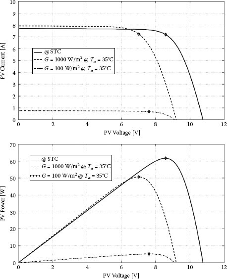
FIGURE 1.11
Current vs. voltage and power vs. voltage curves of a string of PV cells in STC and outdoor environmental conditions.

1.6    The Lambert W Function for Modeling a PV Field

1.6.1    PV Generator Working in Uniform Conditions

The fact that Equation (1.10) does not admit an explicit solution represents a significant limitation, not only in the identification of the model parameters but also in the simulation of PV systems, as the operating point of the PV unit can be obtained only at the price of the solution of the nonlinear equation (1.10). Such limitation can be overcome by using the Lambert W function. In [10] many details and useful references about the Lambert W function can be found. The use of the Lambert W function leads to the following expression:

TABLE 1.4

Suntech STP245S-20/Wd: Data Sheet Values

PV Array	Values in STC Conditions
Short-circuit current ISTC	8.52 A
Open-circuit voltage VOC	37.3 V
MPP current IMPP	8.04 A
MPP voltage VMPP	30.5 V
Temperature coefficient of ISC (αI)	0.05%/°C
Temperature coefficient of VOC (αV)	−0.34%/°C
NOCT	45°C
Number of cells in series	60

TABLE 1.5

Parameters of the PV Circuital Model

Parameters	Values
Iph	8.52 A
Rs	0.2584 Ω
R	1278.1 Ω
C0	286.0364 A/K3
η	1.0457

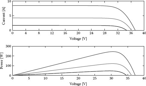
FIGURE 1.12
Current vs. voltage and power vs. voltage curves of the Suntech PV panel: effect of irradiation.

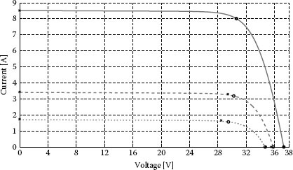
FIGURE 1.13
Current vs. voltage curves of the Suntech PV panel. Continuous line G = 1000 W/m², dashed line G = 400 W/m², dash-dotted line G = 200 W/m². Crosses are experimental points and dots are estimated points.

$I=\frac{R_p\cdot \left(I_{ph}+I_{sat}\right)-V}{R_s+R_p}-\frac{\text{η}\cdot V_t}{R_s}\cdot LambertW\left(\text{θ}\right)$

(1.57)

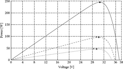
FIGURE 1.14
Power vs. voltage curves of the Suntech PV panel. Continuous line G = 1000 W/m², dashed line G = 400 W/m², dash-dotted line G = 200 W/m². Crosses are experimental points and dots are estimated points.

where

$\text{θ}=\frac{\left(R_p//R_s\right)\cdot I_{sat}\cdot e^{\frac{R_p\cdot R_s\cdot \left(I_{ph}+I_{sat}\right)+R_p\cdot V}{\text{η}\cdot V_t\cdot \left(R_p+R_s\right)}}}{\text{η}\cdot V_t}$

(1.58)

It is easy to see that the expression is now explicit, so that for any value of the PV voltage V the corresponding value of the PV current I can be calculated straightforwardly, the Lambert W function being calculated by means of a series expansion [10]. Similarly, the voltage can be explicitly expressed as a function of the current as well.

Needless to say, such a model can be applied to any level of the PV field because, provided that all the cells in all the modules in all the strings of the PV field operate in exactly the same conditions, the parameters appearing in (1.57) and (1.58) can be scaled accordingly.

Unfortunately, in nonuniform operating conditions, the model and the explicit expression (1.57) are not so simple and scalable, so that a different analysis approach must be adopted.

1.6.2    Modeling a Mismatched PV Generator

As discussed in the preceding sections, mismatching conditions occur when a part of the PV generator works in conditions that are different from those of the remaining part of the generator itself. The occurrence of this situation is due to shadowing or to a significant difference in the physical parameters characterizing the cells. Some approaches have been presented in literature, e.g., in [7, 12, 13], to analyze such situations.

The analysis approach discussed in this section refers to a single PV string made of a number of PV modules connected in series. Each PV module is supposed to be a number of equal cells connected in series and working in the same temperature and irradiance conditions. The cells in the PV module are supposed to be protected by a bypass diode connected in antiparallel, as in Figure 1.1. The approach can be applied to any number of strings connected in parallel.

The group of cells in each module, working in homogeneous conditions, is represented by the equivalent circuit in Figure 1.8 and modeled by the corresponding equation (1.10). Nevertheless, the modules in the string are characterized by different sets of parameters, accounting for nonuniformities in terms of irradiance, temperature, or manufacturing tolerances. In order to have a compact model, it is useful to embed the bypass diode model in a complete model describing the whole PV module, including the cells and the bypass diode, as shown in Figure 1.15.

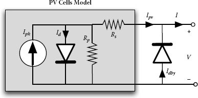
FIGURE 1.15
Equivalent circuit of a PV module with its own bypass diode.

The nonlinear characteristic equation of the bypass diode is given by the Shockley equation:

$I_{dby}=I_{sat,dby}\cdot \left(e^{-\frac{V}{\text{η}dby{V}_{t,dby}}}-1\right)$

(1.59)

Merging (1.10) and (1.59) provides the following nonlinear and implicit equation:

$I=I_{ph}-I_{sat}\cdot \left[e^{\frac{V+I\cdot R_s}{\text{η}{V}_t}}-1\right]-\frac{V+I\cdot R_s}{R_p}+I_{sat,dby}\cdot \left(e^{-\frac{V}{\text{η}dby{V}_{t,dby}}}-1\right)$

(1.60)

Once again, the Lambert W function is useful to put (1.60) into explicit form. The whole module, including the group of cells and the bypass diode, is then described by the following explicit equation, which gives the value of the current of the building block shown in Figure 1.15 as a function of the voltage at its terminals:

$I=\frac{\left[R_p\cdot \left(I_{ph}+I_{sat}\right)-V\right]}{R_s+R_p}+I_{sat,dby}\cdot \left(e^{-\frac{V}{\text{η}dby{V}_{t,dby}}}-1\right)-\frac{\text{η}{V}_t}{R_s}\cdot lambertW\left(\text{θ}\right)$

(1.61)

where θ is given in (1.58).

The mismatched string is made of a series of elements depicted as in Figure 1.15, each one working in certain irradiation and temperature conditions and characterized by given physical parameters that are different from those of the other elements of the string. The string is sketched in Figure 1.16, where each block contains one module depicted in Figure 1.15 and described by Equation (1.61). A blocking diode terminates the string, to avoid the current flowing back from the other strings connected in parallel or, especially in stand-alone applications, from the storage element (e.g., battery).

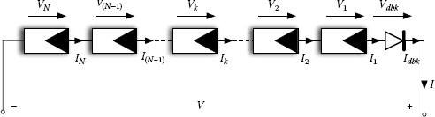
FIGURE 1.16
String of PV modules with blocking diode.

Applying Kirchhoff’s laws, the nonlinear system of Equation (1.62) results:

$\{\begin{array}{l}{V}_1+V_2+\cdot \cdot \cdot +V_k+\cdot \cdot \cdot +V_{N-1}+V_N+V_{dbk}-V=0\\ I_1\left(V_1\right)-I_2\left(V_2\right)=0\\ I_1\left(V_1\right)-I_3\left(V_3\right)=0\\ \cdot \cdot \cdot \\ I_1\left(V_1\right)-I_k\left(V_k\right)=0\\ \cdot \cdot \cdot \\ I_1\left(V_1\right)-I_{N-1}\left(V_{N-1}\right)=0\\ I_1\left(V_1\right)-I_N\left(V_N\right)=0\\ I_1\left(V_1\right)-I_{dbk}\left(V_{dbk}\right)=0\end{array}$

(1.62)

As the model is based on a voltage-driven approach, given any value of the voltage V of the string, the corresponding current has to be calculated through the solution of the system in (1.62). The (N + 1) unknowns {V₁, V₂, …, V_k, …, V_N−1, V_N, V_dbk} are the voltages across the modules and the blocking diode. The N currents appearing in (1.62) are given by (1.61) for the PV modules and by (1.63) for the blocking diode:

$I_{dbk}=I_{sat,dbk}\cdot \left(e^{\frac{V_{dbk}}{V_{t,dbk}}}-1\right)$

(1.63)

All the parameters appearing in the system in (1.62), from the second up to the (N + 1)-th equation, are different for each PV panel. The nonlinear system (1.62) can be solved by using the Newton-Raphson method. It is shown below that the way the system has been written brings significant advantages for its numerical solution. In fact, the equations from the second to the (N + 1)-th have been all referred to the first module. Such a choice simplifies the expression of the Jacobian matrix of the system of equations (1.62).

Thanks to Lambert W function properties, the first derivative of the panel current with respect to the terminal voltage can be calculated in explicit form starting from Equation (1.61). In particular, Equation (1.64) provides the derivative of the lambertW(θ) function with respect to θ,

$\frac{dlambertW\left(\text{θ}\right)}{d\text{θ}}=\frac{1}{\left[1+lambertW\left(\text{θ}\right)\right]\cdot e^{lambertW\left(\text{θ}\right)}}=\frac{lambertW\left(\text{θ}\right)}{\left[1+lambertW\left(\text{θ}\right)\right]\cdot \text{θ}}$

(1.64)

whereas Equation (1.65) provides the expression of the derivative of I with respect to V at the panel terminals.

$\frac{\partial I}{\partial V}=-\frac{1}{R_s+R_p}-\frac{I_{sat,dby}}{V_{t,dby}}\cdot e^{-\frac{V}{V_{t,dby}}}-\frac{R_p}{R_s\cdot \left(R_s+R_p\right)}\cdot lambertW\left(\text{θ}\right)$

(1.65)

In this way, both the PV current and its derivative with respect to the PV voltage have been expressed in closed form as functions of the sole voltage V at the terminals.

Thanks to (1.10) it is possible to obtain each term of the Jacobian matrix J, to be inverted at each iteration of the Newton-Raphson-based algorithm, as a function of the unknowns. The Jacobian matrix structure reported in (1.66) puts in evidence that it is sparse and shows a pattern that is characteristic of doubly bordered and diagonal square matrices, also known as arrow-up matrix. It is

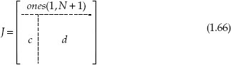
where ones(1, N + 1) is a (N + 1) columns row vector with all the elements equal to 1, c is a column vector of N rows equal to

$c=\frac{\partial I_1}{\partial V_1}\cdot ones\left(N,1\right)$

(1.67)

ones(N, 1) is a N rows column vector with all the elements equal to 1, and

$d=diag\left(\frac{\partial I_1}{\partial V_1},\frac{\partial I_2}{\partial V_2},\cdot \cdot \cdot ,\frac{\partial I_k}{\partial V_k},\cdot \cdot \cdot ,\frac{\partial I_{N-1}}{\partial V_{N-1}},\frac{\partial I_N}{\partial V_N},\frac{\partial I_{dbk}}{\partial V_{dbk}}\right)$

(1.68)

is a diagonal matrix of size N.

The first row is composed by (N + 1) constants, while all the other rows require the evaluation of ∂I₁/∂V₁ and the calculation of another derivative. As a whole, the evaluation of the system (1.62) requires N times the use of Equation (1.61) and 1 times Equation (1.63); the calculation of the Jacobian matrix requires N evaluations of Equation (1.65) and one evaluation of Equation (1.69).

$\frac{\partial I_{dbk}}{\partial V_{dbk}}=\frac{I_{sat,dbk}}{V_{t,dbk}}\cdot e^{-\frac{V_{dbk}}{V_{t,dbk}}}$

(1.69)

Such features are useful in terms of both memory requirements during the simulation and computation time.

Finally, it must be pointed out that Equation (1.65) allows to express in a closed form, and without neglecting any parameter appearing in the model, the differential conductance of the PV generator, which is the slope of the tangent to the I-V curve in the desired operating point. It is a negative value that is of fundamental importance for the best design of the power processing system that takes the PV power at its input and delivers it to the load or the grid. The main role of the differential conductance will be in the determination of the small signal model of the whole system, including the PV generator and the switching converter performing the maximum power point tracking function. This model allows us to design the best dynamic performances for the tracking function. It is also worth noting that the differential conductance (1.65) has a time-varying value, because of its dependence on the irradiance and temperature values.

1.7    Example

In this example the analysis of a PV generator structure is analyzed in presence of nonuniform irradiation conditions. Two identical modules connected in series have been considered, one subjected to a normalized irradiation level equal to G₁/G_max = 1 and the other to a normalized irradiation level G₂/G_max = 0.1. If the two modules were subjected to the same G = 1, the P-V characteristic would be that shown in Figure 1.17. The plot has been obtained by multiplying by 2 the voltage values of the characteristic curve of one of the two identical modules.

In the presence of a significant difference in the irradiance value, the method described in Section 1.6 has been used. The same analysis has been repeated many times, thus assigning a number of samples to the total array voltage V in (1.62) in the range of normalized voltage between 0 and 1. Figure 1.18 shows how dramatically the P-V curve has changed, with the presence of two maximum power points, the absolute MPP occurring at a low voltage level and the relative MPP being placed at a voltage quite close to that one at which the unique MPP occurred in the uniform case shown in Figure 1.17.

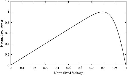
FIGURE 1.17
PV characteristic in uniform conditions.

The presence of the two peaks can be explained in a simple way by looking at the I-V characteristic reported in Figure 1.19. At a low voltage level, the current I₁ produced by the string of PV cells receiving the highest irradiation is larger than the I₂ the other string is able to produce, so that the bypass diode of the second module starts to conduct the difference current I_{1 −} I₂. The diode, during its conduction, inverts the voltage at the terminals of the second PV string, which generates a nonzero current. As a consequence, the second string absorbs an electrical power that is the product of the current it generates by the conduction voltage of the bypass diode. Due to the few hundreds of millivolts of the latter, the dissipated power is limited to a low value. In uniform, yet reduced, irradiation conditions over the cells of the module, the less irradiated string is not subjected to hot spot phenomena. In such conditions, the whole system produces an electrical power that is the power produced by the first string from which the power absorbed by the second string and the power dissipated by the second bypass diode must be subtracted.

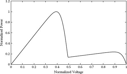
FIGURE 1.18
P-V characteristic in mismatched conditions.

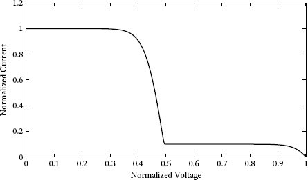
FIGURE 1.19
I-V characteristic in mismatched conditions.

Truly speaking, the bypass diode is helpful if the whole second string is subjected to G₂, but unfortunately, if some cells of this string receive a very low irradiation level, due to a shadowing body lying on its surface, disruptive phenomena can occur. Indeed, as pointed out in literature (e.g., in [2]), if few cells in a module are affected by a deep shadowing effect with respect to many others fully illuminated, hot spot phenomena can take place. The shadowed cells are forced to work at a very negative voltage, but they conduct a significant forward current, imposed by the other cells that receive a high irradiation. The bypass diode does not go into conduction because the large forward voltage of the illuminated cells is partially compensated by the deep negative voltage of the shadowed ones. In such conditions the risk of a permanent damage of the shadowed cells is very high.

As shown in Figures 1.19 and 1.20, at a value of the normalized voltage approximately equal to 0.5, in the example considered herein, the current I₁ drops and reaches the value I₂, so that the current in the second bypass diode becomes zero and in the two PV strings the same current flows. This condition holds up to the total voltage V being equal to the sum of the open-circuit voltages of the two PV strings.

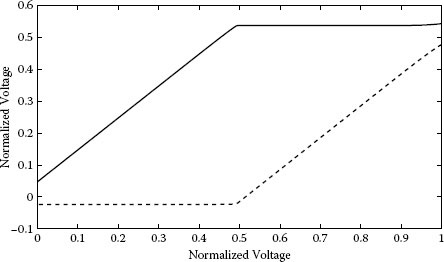
FIGURE 1.20
Voltage across the two modules vs. total voltage. Horizontal axis: voltage on the series connection of the two modules. Vertical axis: voltage on each module. Continuous line: fully irradiated module. Dashed line: shadowed module.

References

1.  M.G. Villalva, J.R. Gazoli, and E.R. Filho. Comprehensive approach to modeling and simulation of photovoltaic arrays. IEEE Transactions on Power Electronics, 24(5):1198–1208, 2009.

2.  U. Eicker. Solar technologies for buildings. Wiley, West Sussex, UK, 2003.

3.  B. Bletterie, R. Bruendlinger, and S. Spielauer. Quantifying dynamic MPPT performance under realistic conditions first test results—The way forward. In Proceedings of 21st European Photovoltaic Solar Energy Conference and Exhibition, 2006, pp. 2347–2351.

4.  J.W. Bishop. Computer simulation of the effects of electrical mismatches in photovoltaic cell interconnection circuits. Solar Cells, 25:73–89, 1988.

5.  D. Sera, R. Teodorescu, and P. Rodriguez. PV panel model based on datasheet values. In Proceedings of the IEEE International Symposium on Electronics, June 2007, pp. 2392–2396.

6.  A. Chatterjee, A. Keyhani, and D. Kapoor. Identification of photovoltaic source models. IEEE Transactions on Energy Conversion, 26(3):883–889, 2011.

7  Y.-J. Wang and P.-C. Hsu. Analytical modelling of partial shading and different orientation of photovoltaic modules. IET Renewable Power Generation, 4(3):272–282, 2010.

8.  J.A. Gow and C.D. Manning. Development of a photovoltaic array model for use in power electronics simulation studies. IEE Proceedings-Electric Power Applications, 146(2):193–200, 1999.

9.  E. Saloux, A. Teyssedou, and M. Sorin. Explicit model of photovoltaic panels to determine voltages and currents at the maximum power point. Solar Energy, 85:713–722, 2011.

10.  Weisstein, Eric W. Lambert W-Function. From MathWorld—A Wolfram Web Resource. http://mathworld.wolfram.com/LambertW-Function.html.

11.  F. Ghani and M. Duke. Numerical determination of parasitic resistances of a solar cell using the lambert w-function. Solar Energy, 85(9):2386–2394, 2011.

12.  G. Petrone and C.A. Ramos-Paja. Modeling of photovoltaic fields in mismatched conditions for energy yield evaluations. In Electric Power Systems Research, 2011, pp. 1003–1013.

13.  G. Petrone, G. Spagnuolo, and M. Vitelli. Analytical model of mismatched photovoltaic fields by means of lambert w-function. In Solar Energy Materials and Solar Cells, 2007, pp. 1652–1657.

^*  MATLAB^® is a registered trademark of The MathWorks, Inc.

^*  The nominal operating cell temperature (NOCT) is defined as the temperature reached by open-circuit cells in a module under the following conditions: irradiance on cell surface G = 800 W/m², air temperature T_a = 20°C, wind velocity = 1 m/s, mounting = open back side.

^*  For crystalline silicon: E_gap = 1.124 eV = 1.8·10⁻¹⁹ J.