
Chapter 10
Survival Analysis
Frédéric Planchet
ISFA - Université de Lyon 1, France — Prim'Act
Lyon, France
Pierre-E. Thérond
ISFA - Université de Lyon 1, Galea & Associés
Lyon, France
10.1 Introduction
The purpose of this chapter dedicated to duration models is to provide operational tools with R to implement them effectively in the context of their most common use in insurance. After a brief reminder of the theoretical context, examples that illustrate the practical implementation of the R functions concerned are provided. Each example begins with a reminder of the underlying theory and the associated code is commented. The reader interested in a complete presentation of theoretical concepts may consult for example, Planchet & Thérond (2011) or Martinussen & Scheike (2006).
We will here consider the following framework, which is very often used in actuarial problems:
- From the data, we must compute crude estimators ˆqx of conditional exit (death for example) probabilities qx;
- The crude rates must then be graduated;
- Finally, it is essential to validate that the model and the data are consistent.
These three steps are described later in this chapter.
Let us consider a positive random variable T. In the following, we denote
F(t)=ℙ(T≤t)
its cumulative distribution function. When F is differentiable, we will denote f, the density function of T defined by
f(t)=ddtF(t)
The survival function of T is
S(t)=1−F(t)
We can define the sfd R function in order to plot survival distribution functions:
> sdf <- function (x)
+ {
+ x <— sort(x)
+ n <— length(x)
+ if (n < 1)
+ stop("'x' must have 1 or more non-missing values")
+ vals <- unique(x)
+ rval <- approxfun(vals, 1-cumsum(tabulate(match(x, vals)))/n,
+ method = "constant", yleft = 1, yright = 0,
+ f = 0, ties = "ordered")
+ class(rval) <- c("ecdf", "stepfun", class(rval))
+ assign("nobs", n, envir = environment(rval))
+ attr(rval, "call") <- sys.call()
+ rval
+}
The survival function S is non-increasing such that S(0) = 1 and limt−∞S(t) = 0 . The survival expectation is easily expressed with S by
?(T)=∫∞0tdF(t)=−∫∞0tdS(t)=∫∞0S(t)dt
The variance of T may be expressed as
Var(T)=2∫∞0tS(t)dt−?T2
In the following, we will consider the conditional survival function defined by
Su(t)=ℙ(T>u+t|T>u)=ℙ(T>t+u)ℙ(T>u)=S(u+t)S(u)
If we consider that T is the lifetime of a policyholder, Su(t) represents the probability that he survives until time t + u considering that he is alive at time t.
When F is differentiable, we define the hazard function by
h(t)=f(t)S(t)=−S′(t)S(t)=−ddtlogS(t)
As a consequence of the definition, S can be expressed in h terms as
S(t)=exp−∫t0h(s)ds.
The cumulative hazard function of T is defined by
H(t)=∫t0h(s)ds.
We immediately have S(t) = exp (..H(t)) . We can observe that H(T) is a random variable exponentially distributed with parameter λ=1 because
ℙ(H(T)>x)=ℙ(T>H−1(x))=S(H−1(x))
=exp{−H(H−1(x))}=e−x,x≥0
In this chapter, two sets of data are used:
- Mortality portfolio (Sections 10.2 and 10.3);
- Disability portfolio (Section 10.4).
But before that, let us mention the specificities of incomplete data.
10.2 Working with Incomplete Data
The aim of this section is to examine how to import and which data manipulations to operate in order to build a survival model. The basic data of this kind of model are incomplete data (i.e., truncated or censored observations).
We assume in the remainder of this chapter that we have individual data on a duration phenomenon. Thus, there is statistical material for estimating the different laws of interest: mortality, time in disability, survival of an annuitant, etc. Because of the conditions for collecting data, right-censored observations are available (due to the presence of individuals at risk at the time of extraction) and left-truncated (because tracking individuals starts generally not from the beginning of the modeled state). From a formal point of view, we have a sample of survival times (X1,...,Xn) and a second independent sample of variables of censorship (C1,...,Cn) . Instead of observing directly (X1,..., Xn) , we observe
Y1 = (T1,D1) ,⋯, Yn = (Tn,Dn),
where Ti=Xi∧i and
Di ={1, if xi≤ Ci, 0, if xi ≤ Ci.
Consider, for instance, exponential durations X, and deterministic (and constant) censorship:
> set.seed(1)
> n <- 20; X <- rexp(n); C <- rep(2,n)
> T <- apply(data.frame(X,C),1,min)
> D <- (T==X)*1
> SampleData <- Surv(T,D)
If we plot the empirical distribution function on (censored) survival times, we get the graphic on the left of of Figure 10.1.
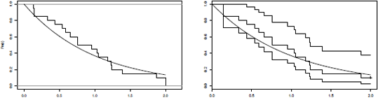
Survival distribution function: empirical distribution from censored survival times, and Kaplan-Meier's correction.
> t <- seq(0,2,by=.01)
> plot(sdf(T),verticals=TRUE,do.points = FALSE,main="")
> lines(t,exp(-t),lwd=2)
The estimation of the survival function is obtained using
> plot(survfit(Surv(T,D)~1))
> lines(t,exp(-t),lwd=2)
See graphic on the right of Figure 10.1
In addition, the data are left-truncated, that is to say, we did observe individuals whose time of entry into the observation is Tj ≥ Ei .
10.2.1 Data Importation and Some Statistics
In this subsection, we consider a .csv file containing the incomplete data. We are going to import it; to build the variables, we will have to use for constructing a survival model, and to identify and delete any anomalies in the database.
A key point here is to define the so-called observation period: we have to know the earliest and the latest dates for which the information is complete.
At first we import the data:
> data=read.table("data\DataMortality.csv",header=TRUE,sep=";")
Then we convert the dates that are in the database.
> data$BirthDate <- as.Date(data$BirthDate,"%d/%m/%Y")
> data$BegDate <- as.Date(data$BegDate,"%d/%m/%Y")
> data$EndDate <- as.Date(data$EndDate,"%d/%m/%Y")
Let us observe some preliminary statistics using the summary function:
> summary(data)
Id BirthDate Sex BegDate
Min. : 1 Min. :1911-10-13 F: 43755 Min. :1935-05-01
1st Qu.: 40238 1st Qu.:1947-05-15 M:117194 1st Qu.:1976-03-01
Median : 80475 Median :1961-03-19 Median :1991-09-01
Mean : 80475 Mean :1960-02-27 Mean :1988-11-15
3rd Qu.:120712 3rd Qu.:1975-08-01 3rd Qu.:2003-02-01
Max. :160949 Max. :1994-12-07 Max. :2012-03-01
EndDate Status GuarCode GuarOption
Min. :1995-05-02 autre : 407 DCC1 :10023 A01:141042
1st Qu.:2007-12-31 encours :152610 DCE1 : 4 B01: 9880
Median :2009-11-30 deceased: 7932 DCP65: 12 C01: 1561
Mean :2011-03-24 DCPA1: 9868 C02: 8462
3rd Qu.:2011-10-31 DCSTA: 85101 E02: 4
Max. :2057-12-31 DCST R:55941
Before building the appropriate database, it is useful to test the consistency of the database with some tests such as
- Number of rows with the birth date posterior to the inception date:
> nrow(subset(data,data$BirthDate>data$BegDate))
[1] 0
- Number of rows with a deceased status and without any exit date:
> nrow(subset(data, data$Status=="deceased" & is.na(data$EndDate)))
[1] 0
10.2.2 Building the Appropriate Database
Let us suppose that we choose the following observation period for the study: from 2009 to 2011. Let us define the following parameters:
> BegObsDate <- as.Date("01/01/2009","%d/%m%Y")
> EndObsDate <- as.Date("31/12/2011","%d/%m/%Y")
We are going to select the data observed during the observation period. In the first time, we define the boundaries of the observation period:
> BegObsDate <- as.Date("01/01/2009","%d/%m/%Y")
> EndObsDate <- as.Date("31/12/2011","%d/%m/%Y")
Then we compute for each observation the beginning and ending dates of observation:
> data$BegObs <- pmax(BegObsDate, data$BegDate)
> data$EndObs <- pmin(EndObsDate, data$EndDate)
The true exits are those for which the death time is within the observation period:
> data$non_censored[(data$Status=="deceased")&
+ (data$EndDate<=EndObsDate)] <- TRUE
> data$non_censored[(data$Status!="deceased")|
+ (data$EndDate>EndObsDate)] <- FALSE
Finally, we do not keep in the database the policyholder with
- An exit date prior to the first observation date, or
- An inception date posterior to the last observation date.
> data_obs <- subset(data,
+ (data$EndObs>=BegObsDate) & (data$BegObs<=EndObsDate))
For each policyholder, we calculate the ages at the observation beginning and ending:
> data_obs$BegAge <- as.double(
+ difftime(data_obs$BegObs,data_obs$BirthDate))/365.25
> data_obs$EndAge <- as.double(
+ difftime(data_obs$EndObs,data_obs$BirthDate))/365.25
Now we are going to build two subsets for male and female observations and determine a (nonweighted) sex-ratio:
> data_obsH=subset(data_obs,(data_obs$Sex=="M"))
> data_obsF=subset(data_obs,(data_obs$Sex=="F"))
> print(paste("Sex-ratio : ",nrow(data_obsH)/nrow(data_obs)))
[1] "Sex-ratio : 0.512871549893843"
Now we have in our hands a dataframe object with all the variables we need to build a survival model.
10.2.3 Some Descriptive Statistics
We are now going to build some variables and compute some statistics we will later use in order to check the survival model.
We begin by computing the number of true exits (e.g., deaths for a mortality risk) by age and year during the observation period:
> BegDateYear <- as.Date(
+ c("01/01/2009","01/01/2010","01/01/2011","01/01/2012"),"%d/%m/%Y")
In order to do that, we create a data.frame with the only observations of true exit (just a matter of computing time):
> data_TrueExit <- subset(data_obs, data_obs$non_censored==TRUE)
Then we build a dataframe TrueExitNumber of size
- Rows: the number of considered ages
- Columns: one for the total on the observation period plus one per year in this period (4 in our example)
> TrueExitNumber <- as.data.frame(matrix(nrow = 121, ncol =5))
> colnames(TrueExitNumber) <-
+ c("Age","Total","2009","2010","2011")
> for (x in 0:120){
+ TrueExitNumber[x+1,1] <- x
+ TrueExitNumber[x+1,2] <- sum(floor(data_TrueExit$EndAge)==x)
+ TrueExitNumber[x+1,3] <- sum((floor(data_TrueExit$EndAge)==x) &
+ (data_TrueExit$EndDate < BegDateYear[2]))
+ TrueExitNumber[x+1,4] <- sum((floor(data_TrueExit$EndAge)==x) &
+ (data_TrueExit$EndDate < BegDateYear[3]))
+ TrueExitNumber[x+1,5] <- sum((floor(data_TrueExit$EndAge)==x) &
+ (data_TrueExit$EndDate < BegDateYear[4]))
+}
> TrueExitNumber[, 5]=TrueExitNumber[,5]-TrueExitNumber[,4]
We control the number of true exits
> sum(TrueExitNumber[,2])
[1] 4458
Now we want to build some exposures for each observation year and each age. We first have to determine the age of each policyholder, both at the beginning and the ending of each observation year (only the code for the first year is disclosed below).
> data_obs$BegDate2009 <- BegDateYear[1]
> data_obs$BegDate2009[
+ (data_obs$BegDate>=BegDateYear[1])&(data_obs$BegDate<BegDateYear[2])] <-
+ data_obs$BegDate[
+ (data_obs$BegDate>=BegDateYear[1])&(data_obs$BegDate<BegDateYear[2])]
> is.na(data_obs$BegDate2009) <-
+ (data_obs$BegDate>=BegDateYear[2])|(data_obs$EndDate<BegDateYear[1])
> data_obs$BegAge2009 <-
+ as.double(data_obs$BegDate2009 - data_obs$BirthDate)/365.25
> summary(data_obs$BegAge2009)
Min. 1st Qu. Median Mean 3rd Qu. Max. NA's
18.17 36.08 56.23 54.14 65.74 96.97 777
We follow the same way for the end age:
> data_obs$EndDate2009 <- BegDateYear[2]-1
> data_obs$EndDate2009[(data_obs$EndDate<BegDateYear[2]) & data_obs$non_censored] <-
+ data_obs$EndDate[(data_obs$EndDate<BegDateYear[2]) & data_obs$non_censored]
> is.na(data_obs$EndDate2009) <-
+ (data_obs$BegDate>=BegDateYear[2])|(data_obs$EndDate<BegDateYear[1])
> data_obs$EndAge2009 <-
+ as.double(data_obs$EndDate2009 - data_obs$BirthDate)/365.25
> summary(data_obs$EndAge2009)
Min. 1st Qu. Median Mean 3rd Qu. Max. NA's
18.52 37.06 57.20 55.09 66.73 97.97 777
Now we have to determine, for each observation year and each age, the observation time of each policyholder. In a first step, we create an ExpoNumber variable and three subsets of data_obs (one for each observation year):
> ExpoNumber <- as.data.frame(matrix(nrow = 121, ncol = 5))
> colnames(ExpoNumber) <- c("Age","Total","2009","2010","2011")
> data_obs2009 <- subset(data_obs,!(is.na(data_obs$BegDate2009)))
> data_obs2010 <- subset(data_obs,!(is.na(data_obs$BegDate2010)))
> data_obs2011 <- subset(data_obs,!(is.na(data_obs$BegDate2011)))
> for (x in 0:120){
+ ExpoNumber[x,1] <- x
+ ExpoNumber[x,3] <- sum(data_obs2009$EndAge2009[
+ (floor(data_obs2009$BegAge2009)==x)&(floor(data_obs2009$EndAge2009)==x)]
+ - data_obs2009$BegAge2009[
+ (floor(data_obs2009$BegAge2009)==x)&(floor(data_obs2009$EndAge2009)==x)])
+ ExpoNumber[x,3] <- ExpoNumber[x,3]
+sum(x+1-data_obs2009$BegAge2009[(floor(data_obs2009$BegAge2009)==x)&
+(floor(data_obs2009$EndAge2009)==x+1)])
+ ExpoNumber[x,3] <- ExpoNumber[x,3] + sum(data_obs2009$EndAge2009[
+ (floor(data_obs2009$BegAge2009)==x-1)&(floor(data_obs2009$EndAge2009)==x)]-x)
+ ExpoNumber[x,4] <-sum(data_obs2010$EndAge2010[
+ (floor(data_obs2010$BegAge2010)==x)&(floor(data_obs2010$EndAge2010)==x)]- + data_obs2010$BegAge2010[
+ (floor(data_obs2010$BegAge2010)==x)&(floor(data_obs2010$EndAge2010)==x)])
+ ExpoNumber[x,4] <- ExpoNumber[x,4] +
+ sum(x+1-data_obs2010$BegAge2010[
+ (floor(data_obs2010$BegAge2010)==x)&(floor(data_obs2010$EndAge2010)==x+1)])
+ ExpoNumber[x,4] <- ExpoNumber[x,4]+ sum(data_obs2010$EndAge2010[
+ (floor(data_obs2010$BegAge2010)==x-1)&(floor(data_obs2010$EndAge2010)==x)]-x)
+ ExpoNumber[x,5] <- sum(data_obs2011$EndAge2011[
+ (floor(data_obs2011$BegAge2011)==x)&(floor(data_obs2011$EndAge2011)==x)] - + data_obs2011$BegAge2011[
+ (floor(data_obs2011$BegAge2011)==x)&(floor(data_obs2011$EndAge2011)==x)])
+ ExpoNumber[x,5] <- ExpoNumber[x,5] +
+ sum(x+1-data_obs2011$BegAge2011[(floor(data_obs2011$BegAge2011)==x)&
+ (floor(data_obs2011$EndAge2011)==x+1)])
+ ExpoNumber[x,5] <- ExpoNumber[x,5]+sum(data_obs2011$EndAge2011[
+ (floor(data_obs2011$BegAge2011)==x-1)&(floor(data_obs2011$EndAge2011)==x)]-x)
+}
> ExpoNumber[,2] <- ExpoNumber[,3]+ExpoNumber[,4]+ExpoNumber[,5]
Now we can create some graphics (see Figures 10.2, 10.3 and 10.4):


> xx <- 18:65
> plot(xx,ExpoNumber[xx+1,2],type="h",lwd=2,xlab="Age",
+ ylab="Exposure")
> grid(NA,8,lwd=1, col="black",lty=2)
> barplot(TrueExitNumber[xx+1,2],names.arg=xx,xlab="Age",
+ ylim=c(0,100), ylab="Number of deaths")
> grid(NA,10,lwd=1, col="black",lty=2)
We can also use some advanced graphic functions such as barplot2 (from the gplots library):
> TH0002 <- readNamedRegionFromFile("data/TH0002.xlsx",
+ "TH_0002" , header = TRUE)
> ci.l <- pmax(TrueExitNumber[xx+1,2]
+ -1.96*sqrt(TrueExitNumber[xx+1,2]),0)
> ci.u <- TrueExitNumber[xx+1,2]
+ +1.96*sqrt(TrueExitNumber[xx+1,2])
> barplot2(3*TH0002[xx+1,2]*ExpoNumber[xx+1,2],
+ names.arg=xx,col="red",xlab="Age",ylim=c(0,120),
+ plot.ci=TRUE,ci.lwd=2,ci.color="blue",
+ ci.l = ci.l, ci.u = ci.u,
+ plot.grid=TRUE)
We can observe that the underlying population has significantly higher mortality rates than the mortality table.
10.3 Survival Distribution Estimation
The aim of this section is to estimate some survival distributions from data. There are numerous estimators of survival distribution, such as Nelson-Aalen and Hoem estimators
(see Planchet & Thérond (2011)). After introducing the Hoem estimator (also known as actuarial estimator), we will mainly focus on the Kaplan-Meier estimator of the survival function.
10.3.1 Hoem Estimator of the Conditional Rates
The Hoem estimator of the conditional mortality rates consists of dividing the number of deaths at age x by a measure of the exposure at the same age (see Planchet & Therond (2011)).
With the previously introduced R code, it consists of
Hoem <- TrueExitNumber[,2]/ExpoNumber[,2]
10.3.2 Kaplan—Meier Estimator of the Survival Function
Let us denote ˆS the Kaplan-Meier estimator of the (unknown) survival function S which is defined by
ˆSt=Π(1−diri),
where
- The time serial represents the time (or ages) at which a true exit (e.g., a death) is observed,
- di represents the number of true exits (e.g., deaths) at time A, and
- ri represents the exposure just before ti.
The properties of the Kaplan-Meier estimator have been well-studied and it is the unique estimator of the survival function which is consistent.
We will use the survfit function of the survival library to proceed to this estimation:
> library(survival)
> data_km <- subset(data_obs, data_obs$BegAge<data_obs$EndAge)
> w <- survfit(Surv(BegAge,EndAge,non_censored,type="counting")~1,
+ data=data_km, type="kaplan-meier")
w is a surv object. Its main characteristics are obtained by
> print(w)
Call: survfit(formula = Surv(BegAge, EndAge, non_censored,
type = "counting")~1, data = data_km, type = "kaplan-meier")
records n.max n.start events median 0.95LCL 0.95UCL
22598.0 1719.0 0.0 4450.0 60.6 58.9 62.4
> summary(w)
The last instruction enables as to get the values of the estimator at each death time. We can make a graphical representation (see Figure 10.5) of w using the plot function:

> plot(w, mark.time=FALSE, lty=1, xlim=c(20,80),
+ xlab = "Age", ylab = "Survival function", conf.int=TRUE)
From the summary instruction, we can obtain the value of the estimator at desired times (or ages). For example, if we want to compute some conditional mortality rates (qx), we are interested in the value of the Kaplan-Meier estimator at each integer age.
> summary(w, times = c(40:60))
Call: survfit(formula = Surv(BegAge, EndAge, non_censored,
type = "counting")~1, data = data_km, type = "kaplan-meier")
time n.risk n.event survival std.err lower 95% CI upper 95% CI
40 349 77 0.866 0.0144 0.839 0.895
41 308 5 0.853 0.0153 0.824 0.884
42 290 8 0.831 0.0169 0.798 0.864
43 266 7 0.810 0.0182 0.775 0.846
44 273 2 0.804 0.0185 0.769 0.841
45 301 8 0.782 0.0196 0.744 0.821
46 331 6 0.767 0.0201 0.729 0.808
47 351 7 0.751 0.0206 0.712 0.793
48 401 7 0.738 0.0209 0.698 0.780
49 454 7 0.725 0.0210 0.685 0.768
50 550 14 0.706 0.0211 0.666 0.748
51 671 11 0.693 0.0211 0.653 0.736
52 822 10 0.684 0.0210 0.644 0.726
53 960 28 0.663 0.0207 0.623 0.705
54 1167 29 0.645 0.0204 0.606 0.686
55 1267 40 0.624 0.0200 0.586 0.665
56 1156 36 0.605 0.0197 0.567 0.644
57 1224 61 0.575 0.0191 0.538 0.613
58 1269 47 0.553 0.0186 0.518 0.591
59 1435 51 0.532 0.0181 0.498 0.569
60 1573 58 0.512 0.0176 0.479 0.548
Now we are able to determine the conditional mortality rates.
> sum_w <- summary(w, times = c(20:66))
> q_x <- data.frame(nrow = max(sum_w$time), ncol = 2)
> colnames(q_x) <- c("Age","Rate")
> for (x in min(sum_w$time):(max(sum_w$time)-1)){
+ q_x[x,1] <- x
+ q_x[x,2] <- 1
+ sum_w$surv[sum_w$time==x+1]/sum_w$surv[sum_w$time==x]
+}
And to plot them (see Figure 10.5):

> plot(q_x, xlim=c(20,65), ylim=c(0,.06), pch=3)#,
+ xlab = "Age", ylab = "Rates")
> grid(nx=0, ny=6)
We may finally compare them with those obtained by the Hoem estimators (see Figure 10.7).
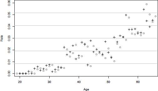
> plot(q_x, xlim=c(20,65), ylim=c(0,.06), pch=3)
> grid(nx=0, ny=6)
> points(Hoem,pch=1)
10.4 Regularization Techniques
When building a table of experience, the first step is the estimation of conditional probabilities of death (exit rate) and this step is essential, both for parametric and nonparametric
approaches. The estimator of the exit rate shows some irregularities, which is legitimate to think that it does not reflect the underlying phenomenon that seeks to measure, but it is the result of imperfect conditions of the experience. The sampling fluctuations thus induce parasite variability in the estimated values. We then want to “adjust” or “smooth” the raw empirical values to represent a more accurate law (unknown) that is to be estimated. The process of revising the original estimate can be conducted in three ways:
- We can fix an a priori form for the underlying law, assuming for example that the hazard function is a Makeham function. This is a fitting approach defined by a parameter distribution.
- We may not find a parametric representation, but simply define a number of treatments to be applied to the original raw data to make them more “smooth.” This is typically the nonparametric methods, for example, Whittaker-Henderson smoothing and its extension in a more general Bayesian framework.
- And we may apply both techniques together, leading to semiparametric models. The Brass model is one of them.
We now assume that we have estimators of the underlying, unknown, conditional exit probabilities (crude rates) and we have to graduate them.
10.4.1 Parametric Adjustment
A very simple approach to address a parametric graduation is to observe that one can often assume that the crude rate estimator at time is normally distributed, that is,
It is then easy to show that when this assumption is true, the optional parameter θ is one that minimizes the function
where Ex denotes the exposure at time x (that is, between x and x +1). The key point is to specify the form of the function .
In the framework of duration models, the most natural way to do that is to make a parametric assumption for the hazard function he and use the link between the hazard function and the conditional exit probabilities
For example, for human mortality, it is well known that the Gompertz-Makeham model
where fits the data relatively well (for not so-aged populations). In this special case, we have
We will now assume that we have the input data for a range . The numerical computation will be done using numerical algorithms like Newton-Raphson or a gradient algorithm. Such an algorithm requires the use of well- chosen initial value for θ, not too far from the optimal one.
In the Gompertz-Makeham case, one can observe that
with
Initial values for and can then be computed using a simple linear regression. The programming of this method with R software is based on the qxAdjust function defined as follows:
> qAdjustH_M <- qxAdjust(Q_H,rowSums(expoVentilesH),xMin,xMax,TRUE,"Makeham")
with
> qxAdjust <- function(qxBrut,expo,xMin,xMax,pond,model){
> pInitial <- getValeursInitiales(qxBrut,xMin,xMax)
> f <- function(p){
+ getEcart(qxBrut,expo,xMin,xMax,p[1],p[2],p[3],pond,model)}
> argmin <- constr0ptim(pInitial,f,ui=rbind(c(1,0,0),c(0,1,0),c(0,0,1)), + ci=c(0,0,0),control=list(maxit=10"3),method="Nelder-Mead")$par
> q <- as.vector(0:120)
> for (x in 0:120){
+ q[x+1]=qxModel(model,argmin[1],argmin[2],argmin[3],x)
+}
> list(argmin,q)
+}
As can be seen, this function uses three auxiliary functions:
> qxModel <- function(model,a,b,c,x){
+ if (model=="Thatcher"){q=qxThatcher(b,log(c),a,x)}
+ else if (model=="Makeham") {q=qxMakeham(a,b,c,x)}
+ else {q=qxLogit(a,b,c,x)}
+ if (is.na(q)){0}
+ else {q}
+}
> getValeurslnitiales <- function(qxBrut,xMin,xMax){
+ q <- pmax(qxBrut,10"-10)
+ x <- as.vector(xMin:xMax)
+ y <- log(pmax(abs(q[(xMin+1):(xMax+1)]
+ -q[(xMin+2):(xMax+2)]),10"-10))
+ t <- data.frame(cbind(x,y))
+ d <- lm(y~x,data=t)
+ p <- as.vector(1:3)
+ p[1] <- 2*10~-4
+ p[3] <- exp(d$coefficients[2])
+ p[2] <- max(10"-10,-log(p[3])*exp(d$coefficients[1])/(p[3]-1)"2)
+ return(p)
+} >getEcart <- function(qxBrut,expo,xMin,xMax,a,b,c,pond,model){
+ w <- pmin(1,as.vector(1:120))
+ if (pond & !(model=="Logit")){
+ expo <- expo[1:120]
+ w <- expo/(qxBrut*(1-qxBrut))
+ }
+ else if (pond & (model=="Logit")){
+ expo <- expo[1:120]
+ w <- expo
+ }
+ w[(is.na(w))|(is.infinite(w))]<-0
+ s <- 0
+ for (x in xMin:xMax){
+ s <- s+w[x+1]*(qxModel(model,a,b,c,x)-qxBrut[x+1])"2
+ }
+ s
+}
At least we need the last simple function:
> qxMakeham <- function(a,b,c,x){
+ 1-exp(-a)*exp(-b/log(c)*(c-1)*c"x)
+}
The above graphics show that the Makeham model may not be the best one. We will now illustrate the use of the Brass relational model.
10.4.2 Semiparametric Adjustment: Brass Relational Model
Modeling the function with asmall number of parameters may be too restrictive. A simple solution is to take a larger parameter. We then have to choose a smart way to choose this less-restrictive parameter. It seems quite natural to use another mortality table (for our sample) and to describe the link between this table and the (unknown) mortality table we want to build. The Brass model relies on the assumption that
where the parameter must be fitted. We use the same criterion as previously, that is, we are looking for the value of the parameter , where we denote
It is sufficient to slightly change the code used in the previous section:
> qxAjusteLogit <- function(qxBrut,expo,xMin,xMax,pond,qxRef){
+ modelLogit <- "Logit"
+ f <- function(p){
+ getEcart(qxBrut,expo,xMin,xMax,p[1],p[2],qxRef,pond,modelLogit)} + argmin <- nlm(f,c(1,0))$estimate
+ q <- as.vector(0:120)
+ for (x in 0:120){
+ q[x+1] <- qxModel(modelLogit,argmin[1],argmin[2],qxRef,x)
+ }
+ list(argmin,q)
+}
with
> qxLogit <- function(a,b,q,x){
+ z=exp(b)*(q[x+1]/(1-q[x+1]))"a
+ z/(1+z)
+}
10.4.3 Nonparametric Techniques: Whittaker—Henderson Smoother
The idea of the method of Whittaker-Henderson is to combine a fidelity criterion and a regularity criterion and find the fitted values that minimize the sum of the two criteria.
We fixed weights and we set the following criteria:
- Fidelity: ,
- Regularity: ,
where z is a parameter of the model. The criterion is to minimize a linear combination of fidelity and regularity functions; the weight of each of the two terms is controlled by a second parameter h:
M = F + h S.
One can show that
with Kz the (p - z,p) matrix whose terms are the binomial coefficients of order z whose sign alternates and began positively to peer z. For example, with p = 5 and z = 2, we have
If p = 3 and z = 1, we have one can easily show that .
This leads to
We then compute
and solve the equation
to get the following result:
.
The method of Whittaker-Henderson is very interesting because its extension in dimension two (or more) is simple. First we distinguish the vertical regularity via the operator (which acts on qi,j, j set seen as a series indexed by i) to calculate an index of vertical regularity:
In the same way, we calculate an index of horizontal regularity Sh , and we denote
which must be minimized. The resolution of the optimization problem is made by rearranging the elements to be reduced to a one-dimensional case. We construct the vector u, of size . Similarly, we construct a weight matrix by copying the diagonal lines of the matrix . We denote . We proceed in the same way to define the matrices and . The smoothed values are then obtained by
10.4.3.1 Application
Here is a simple concrete example that illustrates this method. Crude rates are put in a matrix with p = 3 and q = 4.
> TCrude <- read.table("data/Q_Moment_h.txt", sep=";")
> TCrude <- as.numeric(TCrude)
> TCrude <- as.matrix(TCrude)
> q <- ncol(TCrude)
> p <- nrow(TCrude)
> Weights <- matrix(1,p*q,p*q)
We choose z = 2 (vertical regularity index) and y = l (horizontal regularity index), so that we get matrix and matrix:
> U <- matrix(0,q*p,1)
> v <- matrix(0,VertOrder+1)
> h <- matrix(0,HorOrder+1)
> Kv <- matrix(0,(p-VertOrder)*q,q*p)
> Kh <- matrix(0,p*(q-HorOrder),q*p)
> M <- (matrix(0,q*p,q*p))
> W <- matrix(0,q*p,q*p)
> Qsmooth <- matrix(0,p,q)
> Tsmooth <- matrix(0,p,q)
> for (j in 1:q) {
+ for (i in 1:p) {
+ U[(i-1)*q+j,1] <- as.numeric(TCrude[i,j])
+ W[q*(i-1)+j,q*(i-1)+j] <-Weights[i,j]
+ }
+}
> for (k in 0:VertOrder) {
+ v[(k+1),1]=(-1)~(VertOrder-k)*
+ factorial(VertOrder)/(factorial(k)*factorial(VertOrder-k))
+}
> for (j in 1:q) {
+ for (z in 1:(p-VertOrder)) {
+ for (i in 1:(VertOrder+1)) {
+ Kv[z+(j-1)*(p-VertOrder),j+(q)*(i-1)+(z-1)*(q)]=v[i,1]
+ }
+ }
+}
> for (k in 0:HorOrder) {
+ h[(k+1),1]=(-1)~(HorOrder-k)*factorial(HorOrder)
+ /(factorial(HorOrder-k)*factorial(k))
+}
> M <- W+alpha*(t(Kv))%*%Kv+beta*(t(Kh))%*%Kh
> Qsmooth <- solve(M)%*%W%*%U
> for (j in 1:q) {
+ for (i in 1:p) {
+ Tsmooth[i,j]=Qsmooth[(i-1)*q+j,1]
+ }
+}
With the sample data, we get Figure 10.8.

> q <- ncol(TCrude)
> p <- nrow(TCrude)
> x <- matrix(1:p,p,1)
> y <- matrix(1:q,q,1)
> par(mfrow=c(1,2))
> persp(x,y,TCrude,theta=+100,col=brewer.pal(9,"RdYlGn"),
+ xlab="Age",ylab="Duration",main="Crude rates",adj=0.5,font=2)
> persp(x,y,Tsmooth,theta=+100,col=brewer.pal(9,"RdYlGn"),
+ xlab="Age",ylab="Duration",main="Smooth rates",adj=0.5,font=2)
10.5 Modeling Heterogeneity
Heterogeneity is a mixture of populations with different characteristics. It has a significant impact on the perception of the hazard function of the model. For example, a mixture of exponential population (thus constant hazard) leads to a decreasing aggregate hazard function. This phenomenon is called “heterogeneity bias.”
Many models take into account this mixture of laws: frailty models (Vaupel et al. (1979), combined fragility (Barbi (1999)), common shocks models, Cox model (Cox (1972)), additive hazard decomposition (Aalen (1978)), combinations of both, etc. In the context of actuarial models, the Cox model and, more recently, the Aalens one, are widely used, in particular because of their ease of implementation and interpretation, and also because the presence of censorship (right) and truncation (left) are taken into account.
The reference model for proportional hazard is the model of Cox (1972), specified as follows from the hazard function:
So this is a regression model whose coefficients can be estimated by (partial) maximum likelihood. The link with the discrete exit rate is immediate:
The approximation is valid when the exit rate is low. This framework may actually be declined in several ways, depending on how you consider the baseline hazard function:
- If a parameter is specified, one obtains in practice a complete parametric model that one can try to estimate by maximum likelihood.
- If the baseline hazard function is known, one can use least squares methods.
- If one does not specify a priori any particular form for the baseline hazard function, the model is a semiparametric one, which is the framework chosen by Cox.
The hazard function is then of the form
and we can calculate the log-likelihood in the presence of right censoring and left truncation (see Planchet & Therond (2011)):
with k a constant and . For example, if we choose a hazard function based on a Weibull distribution,
.
This case has, in practice, been discussed above and requires no special comment.
10.5.1 Semiparametric Framework: Cox Model
The idea here is to separate the estimation of the heterogeneity parameter on one hand and the baseline hazard function on the other. Cox showed in 1972 that this could be done using the following partial likelihood:
> cox <- coxph(Surv(AncEntree,AncSortie,
+ non_censored,"counting")~Sexe+CSP,data=t)
> summary(cox)
Call:
coxph(formula = Surv(AncEntree, AncSortie,
non_censored, "counting") ~ Sexe + CSP, data = t)
coef exp(coef) se(coef) z p
SexeH 0.1512 1.163 0.00298 50.83 0.0e+00
CSPENSPER -0.0186 0.982 0.00290 -6.41 1.4e-10
CSPCADRES -0.1868 0.830 0.01005 -18.59 0.0e+00
Likelihood ratio test=2864 on 3 df,
p=0 n= 542619, number of events= 520238
There is a test to validate the proportionality assumption underlying the model, based on the Schoenfeld residuals:
> cox.zph(cox)
rho chisq p
SexeH -0.0765 3031 0
CSPENSPER 0.0488 1238 0
CSPCADRES 0.0302 476 0
GLOBAL NA 4784 0
10.5.2 Additive Models
When the proportional hazard hypothesis is not satisfied, we can turn to the additive models (Aalen (1978)), whose general shape is based on the following specification of the hazard function:
.
So, for an individual i, we have
Depending on the assumptions on the model, coefficients can be parametric, semiparametric, or nonparametric. For example, in the nonparametric framework, by introducing the matrix :
and its generalized inverse (see Ben-Israel & Greville (2003) of size :
we know how to estimate the cumulative regression coefficients by
However, we can observe that the volume of calculations to be performed is important, since it is necessary to calculate at every time we observe an uncensored exit. This involves to calculate the inverse (size ) at every time of an uncensored exit, then the matrix products for and finally .
> aa <- aareg(Surv(AncEntree,AncSortie,non_censored,
+ "counting")~CSP,data=t[1:5000,]) Call:
aareg(formula = Surv(AncEntree, AncSortie, non_censored,
"counting") ~ CSP, data = t[1:5000,]) n= 5000
1434 out of 1440 unique event times used
slope coef se(coef) z p
Intercept 0.06310 0.001440 2.73e-05 52.50 0.00000
CSPENSPER -0.00540 -0.000145 4.46e-05 -3.24 0.00118
CSPCADRES -0.00824 -0.000200 6.99e-05 -2.86 0.00420
Chisq=14.73 on 2 df, p=0.00063; test weights=aalen
10.6 Validation of a Survival Model
To validate a model, the most typical approach is to compare the number of observed exits and the number of exits from the model. This comparison is performed over the period of observation. To determine the number of exits estimated by the model, a one-per-capita calculation is performed. The number of predicted exits at time (resp. age) x is equal to the exposure multiplied by the conditional probability of exiting at this time (resp. age).
The calculation conventions may have a significant effect on the output. They are specified here to avoid ambiguity.
The integer age of death is equal to the integer part of the exact age, the latter being calculated by a difference of days and then divided by 365.25.
The exposures are therefore determined on a daily basis by observing, for each insured, the time spent between two ages. The calculation of the contribution v of the insured age x exposure period 01/01/N-31/12/N is performed as follows:
and
with
- - BirthDate refers to the age in days at the end of the observation year N;
- -BirthDate refers to the age in days at the beginning of the observation year N;
- [x] denotes the integer part of x.
To underestimate the bias associated with the above formulas, the age at the end of observation of a person released uncensored (deceased) is taken as equal to the smallest integer greater than the exit age.
Denote by Nx the exposure at age x, Dx the number of deaths in the year of age x people. qx is estimated by . According to the Central Limit theorem,
The asymptotic confidence interval of level is given by
where denotes the percentile function of the standard normal distribution.