![]()
Numerical Algorithms: Equations, Derivatives, Integrals and Differential Equations
8.1 Solving Non-Linear Equations
MATLAB is able to implement a number of algorithms which provide numerical solutions to certain problems which play a central role in the solution of non-linear equations. Such algorithms are easy to construct in MATLAB and are stored as M-files. From previous chapters we know that an M-file is simply a sequence of MATLAB commands or functions that accept arguments and produces output. The M-files are created using the text editor.
8.1.1 The Fixed Point Method for Solving x = g(x)
The fixed point method solves the equation x = g(x), under certain conditions on the function g, using an iterative method that begins with an initial value p0 (a first approximation to the solution) and defines pk+1 = g(pk). The fixed point theorem ensures that, in certain circumstances, this sequence will converges to a solution of the equation x = g(x). In practice the iterative process will stop when the absolute or relative error corresponding to two consecutive iterations is less than a preset value (tolerance). The smaller this value, the better the approximation to the solution of the equation.
This simple iterative method can be implemented using the M-file shown in Figure 8-1.
As an example we solve the following non-linear equation:

![]()
In order to apply the fixed point algorithm we write the equation in the form x = g(x) as follows:
![]()
We will start by finding an approximate solution which will be the first term p0. To plot the x axis and the curve defined by the given equation on the same graph we use the following syntax (see Figure 8-2):
>> fplot ('[x-2^(-x), 0]',[0, 1])

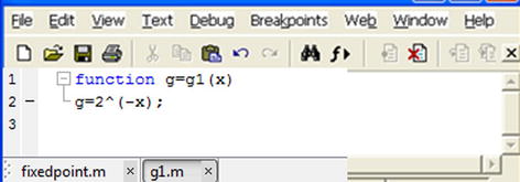
The graph shows that one solution is close to x = 0.6. We can take this value as the initial value. We choose p0 = 0.6. If we consider a tolerance of 0.0001 for a maximum of 1000 iterations, we can solve the problem once we have defined the function g(x) in the M-file g1.m (see Figure 8-3).
We can now solve the equation using the MATLAB syntax:
>> [k, p] = fixedpoint('g1',0.6,0.0001,1000)

k =

    10


p =

    0.6412
We obtain the solution x = 0.6412 at the 1000th iteration. To check if the solution is approximately correct, we must verify that g1(0.6412) is close to 0.6412.
>> g1 (0.6412)

ans =

    0.6412
Thus we observe that the solution is acceptable.
8.1.2 Newton’s Method for Solving the Equation f(x) = 0
Newton’s method (also called the Newton–Raphson method) for solving the equation f(x) = 0, under certain conditions on f, uses the iteration
![]()
for an initial value x0 close to a solution.
The M-file in Figure 8-4 shows a program which solves equations by Newton’s method to a given precision.

As an example we solve the following equation by Newton’s method:
![]()
The function f (x) is defined in the M-file f1.m (see Figure 8-5), and its derivative f'(x) is given in the M-file derf1.m (see Figure 8-6).


We can now solve the equation up to an accuracy of 0.0001 and 0.000001 using the following MATLAB syntax, starting with an initial estimate of 1.5:
>> [x,it]=newton('f1','derf1',1.5,0.0001)

x =

1.6101


it =

2

>> [x,it]=newton('f1','derf1',1.5,0.000001)
x =

1.6100

it =

3
Thus we have obtained the solution x = 1.61 in just 2 iterations for a precision of 0.0001 and in just 3 iterations for a precision of 0.000001.
8.1.3 Schröder’s Method for Solving the Equation f(x)=0
Schröder's method, which is similar to Newton’s method, solves the equation f(x) = 0, under certain conditions on f, via the iteration
![]()
for an initial value x0 close to a solution, and where m is the order of multiplicity of the solution being sought.
The M-file shown in Figure 8-7 gives the function that solves equations by Schröder's method to a given precision.

8.2 Systems of Non-Linear Equations
As for differential equations, it is possible to implement algorithms with MATLAB that solve systems of non-linear equations using classical iterative numerical methods.
Among a diverse collection of existing methods we will consider the Seidel and Newton–Raphson methods.
8.2.1 The Seidel Method
The Seidel method for solving systems of equations is a generalization of the fixed point iterative method for single equations.
In the case of a system of two equations x = g1(x,y) and y = g2(x,y) the terms of the iteration are defined as:
Pk+1= g1(pk,qk) and qk+1= g2(pk,qk).
Similarly, in the case of a system of three equations x=g1(x,y,z),
y = g2(x,y,z) and z = g3(x,y,z) the terms of the iteration are defined as:
pk+1= g1(pk,qk,rk), qk+1= g2(pk,qk,r4) and rk+1= g3(pk,qk,r4).
The M-file shown in Figure 8-8 gives a function which solves systems of equations using Seidel’s method up to a specified accuracy.

8.2.2 The Newton-Raphson Method
The Newton–Raphson method for solving systems of equations is a generalization of Newton’s method for single equations.
The idea behind the algorithm is familiar. The solution of the system of non-linear equations F(X) = 0 is obtained by generating from an initial approximation P0 a sequence of approximations Pk which converges to the solution. Figure 8-9 shows the M-file containing the function which solves systems of equations using the Newton–Raphson method up to a specified degree of accuracy.

As an example we solve the following system of equations by the Newton–Raphson method:

taking as an initial approximation to the solution P = [2 3].
We start by defining the system F(X) = 0 and its Jacobian matrix JF according to the M-files F.m and JF.m shown in Figures 8-10 and 8-11.


Then the system is solved with a tolerance of 0.00001 and with a maximum of 100 iterations using the following MATLAB syntax:
>> [P,it,absoluteerror]=raphson('F','JF',[2 3],0.00001,0.00001,100)

P =

1.9007 0.3112

it =

6

absoluteerror =

8. 8751e-006
The solution obtained in 6 iterations is x = 1.9007, y = 0.3112, with an absolute error of 8.8751e-006.
8.3 Interpolation Methods
There are many different methods available to find an interpolating polynomial that fits a given set of points in the best possible way.
Among the most common methods of interpolation, we have Lagrange polynomial interpolation, Newton polynomial interpolation and Chebyshev approximation.
8.3.1 Lagrange Polynomial Interpolation
The Lagrange interpolating polynomial which passes through the N+1 points (xk yk), k= 0,1,…, N, is defined as follows:

where:

The algorithm for obtaining P and L is easily implemented by the M-file shown in Figure 8-12.

As an example we find the Lagrange interpolating polynomial that passes through the points (2,3), (4,5), (6,5), (7,6), (8,8), (9,7).
We will simply use the following MATLAB syntax:
>> [F, L] = lagrange([2 4 6 7 8 9],[3 5 5 6 8 7])

C =

-0.0185 0.4857 -4.8125 22.2143 -46.6690 38.8000

L =

-0.0006 0.0202 -0.2708 1.7798 -5.7286 7.2000
0.0042 -0.1333 1.6458 -9.6667 26.3500 -25.2000
-0.0208 0.6250 -7.1458 38.3750 -94.8333 84.0000
0.0333 -0.9667 10.6667 -55.3333 132.8000 -115.2000
-0.0208 0.5833 -6.2292 31.4167 -73.7500 63.0000
0.0048 -0.1286 1.3333 -6.5714 15.1619 -12.8000
We can obtain the symbolic form of the polynomial whose coefficients are given by the vector C by using the following MATLAB command:
>> pretty(poly2sym(C))

   31     5    1093731338075689      4   77       3      311     2   19601
- ----   x  + -----------------     x  - ----    x  +    ---    x  - --------    x + 194/5
  1680         2251799813685248          16              14          420
8.3.2 Newton Polynomial Interpolation
The Newton interpolating polynomial that passes through the N+1 points (xk yk) = (xk, f(xk)), k= 0,1,…, N, is defined as follows:
![]()
where:

Obtaining the coefficients C of the interpolating polynomial and the divided difference table D is easily done via the M-file shown in Figure 8-13.

As an example we apply Newton’s method to the same interpolation problem solved by the Lagrange method in the previous section. We will use the following MATLAB syntax:
>> [C, D] = pnewton([2 4 6 7 8 9],[3 5 5 6 8 7])
C =
-0.0185 0.4857 - 4.8125 22.2143 - 46.6690 38.8000
D =
3.0000         0         0         0         0         0
5.0000    1.0000         0         0         0         0
5.0000         0       - 0.2500    0         0         0
6.0000    1.0000         0.3333    0.1167    0         0
8.0000    2.0000         0.5000    0.0417  - 0.0125    0
7.0000  - 1.0000       - 1.5000  - 0.6667  - 0.1417  - 0.0185
The interpolating polynomial in symbolic form is calculated as follows:
>> pretty(poly2sym(C))
    31     5  17   4   77   3   311    2   19601
- ----   x  + --  x  - --  x  + ---   x  - -----    x + 194/5
  1680        35       16       14          420
Observe that the results obtained by both interpolation methods are similar.
8.4 Numerical Derivation Methods
There are various different techniques available for numerical derivation. These are of great importance when developing algorithms to solve problems involving ordinary or partial differential equations.
Among the most common methods for numerical derivation are derivation using limits, derivation using extrapolation and derivation using interpolation on N-1 nodes.
8.4.1 Numerical Derivation via Limits
This method consists in building a sequence of numerical approximations to f' (x) via the generated sequence:

The iterations continue until |Dn+1−Dn|≥|Dn−Dn-1| or |Dn−Dn−1|< tolerance. This approach approximates f'(x) by Dn.
The algorithm to obtain the derivative D is easily implemented by the M-file shown in Figure 8-14.

As an example, we approximate the derivative of the function:


To begin we define the function f in an M-file named funcion (see Figure 8-15). (Note: we use funcion rather than function here since the latter is a protected term in MATLAB.)

The derivative is then given by the following MATLAB command:
>> [L, n] = derivedlim ('funcion', (1-sqrt (5)) / 2,0.01)

L =

1.0000 - 0.7448 0
0.1000 - 2.6045 1.8598
0.0100 - 2.6122 0.0077
0.0010 - 2.6122 0.0000
0.0001 - 2.6122 0.0000

n =
4
Thus we see that the approximate derivative is – 2.6122, which can be checked as follows:
>> f = diff ('sin (cos (x))')

f =

cos (cos (x)) * sin (x) / x ^ 2

>> subs (f, (1-sqrt (5)) / 2).

ans =

   -2.6122
8.4.2 Richardson’s Extrapolation Method
This method involves building numerical approximations to f'(x) via the construction of a table of values D(j, k) with k≤j that yield a final solution to the derivative f' (x) = D(n, n). The values D(j, k) form a lower triangular matrix, the first column of which is defined as:

and the remaining elements are defined by:

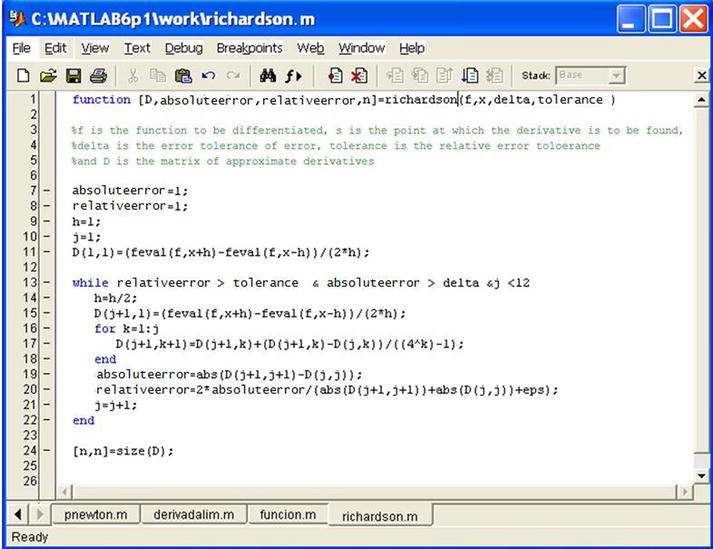
The corresponding algorithm for D is implemented by the M-file shown in Figure 8-16.
As an example, we approximate the derivative of the function:


As the M-file that defines the function f has already been defined in the previous section, we can find the approximate derivative using the MATLAB syntax:
>> [D, relativeerror, absoluteerror, n] = richardson ('funcion', (1-sqrt(5))/2,0.001,0.001)

D =

   -0.7448   0        0        0        0        0
   -1.1335 - 1.2631   0        0        0        0
   -2.3716 - 2.7843 - 2.8857   0        0        0
   -2.5947 - 2.6691 - 2.6614 - 2.6578   0        0
   -2.6107 - 2.6160 - 2.6125 - 2.6117 - 2.6115   0
   -2.6120 - 2.6124 - 2.6122 - 2.6122 - 2.6122 - 2.6122

relativeerror =

  6. 9003e-004

absoluteerror =

  2. 6419e-004

n =
6
Thus we get the same result as before when we used the limit method.
8.4.3 Derivation Using Interpolation (n + 1 Nodes)
This method consists in building the Newton interpolating polynomial of degree N:
![]()
and numerically approximating f'(x0) by P'(x0).
The algorithm for the derivative D is easily implemented by the M-file shown in Figure 8-17.

As an example, we approximate the derivative of the function:


As the M-file that defines the function f has already been constructed in the previous section, we can calculate the approximate derivative using the MATLAB command:
>> [A, df] = nodes([2 4 6 7 8 9],[3 5 5 6 8 7])

A =

3.0000  1.0000  - 0.2500  0.1167  - 0.0125  - 0.0185

df =
-1.4952
8.5 Numerical Integration Methods
Given the difficulty of obtaining an exact primitive for most functions, numerical integration methods are especially important. There are many different ways to numerically approximate definite integrals, among them the trapezium method, Simpson’s method and Romberg’s method (all implemented in MATLAB’s Basic module).
8.5.1 The Trapezium Method
The trapezium method for numerical integration has two variants: the trapezoidal rule and the recursive trapezoidal rule.
The trapezoidal rule approximates the definite integral of the function f(x) between a and b as follows:

calculating f(x) at equidistant points xk = a+kh, k = 0,1,…, M where x0= a and xM = b.
The trapezoidal rule is implemented by the M-file shown in Figure 8-18.

The recursive trapezoidal rule considers the points xk = a+kh, k = 0,1,…, M, where x0 = a and xM = b, dividing the interval [a, b] into 2J = M subintervals of the same size h =(b-a)/2J. We then consider the following recursive formula:


and the integral of the function f(x) between a and b can be calculated as:

using the trapezoidal rule as the number of sub-intervals [a, b] increases, taking at the J-th iteration a set of 2J+ 1 equally spaced points.
The recursive trapezoidal rule is implemented via the M-file shown in Figure 8-19.

As an example, we calculate the following integral using 100 iterations of the recursive trapezoidal rule:

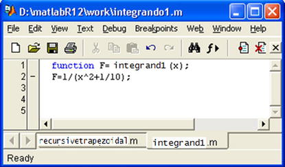
We start by defining the integrand by means of the M-file integrand1.m shown in Figure 8-20.
We then calculate the requested integral as follows:
>> recursivetrapezoidal('integrand1',0,2,14)

ans =

Columns 1 through 4

10.24390243902439   6.03104212860310   4.65685845031979   4.47367657743630

Columns 5 through 8

4.47109102437123 4.47132194954670 4.47138003053334 4.47139455324593

Columns 9 through 12

4.47139818407829 4.47139909179602 4.47139931872606 4.47139937545860

Columns 13 through 15

4.47139938964175 4.47139939318754 4.47139939407398
This shows that after 14 iterations an accurate value for the integral is 4.47139939407398.
We calculate the same integral using the trapezoidal rule, using M = 14, using the following MATLAB command:
>> trapezoidalrule('integrand1',0,2,14)

ans =
4.47100414648074
The result is now the less accurate 4.47100414648074.
8.5.2 Simpson’s Method
Simpson’s method for numerical integration is generally considered in two variants: the simple Simpson’s rule and the composite Simpson's rule.
Simpson’s simple approximation of the definite integral of the function f(x) between the points a and b is the following:

This can be implemented using the M-file shown in Figure 8-21.

The composite Simpson's rule approximates the definite integral of the function f (x) between points a and b as follows:

calculating f(x) at equidistant points xk = a+kh, k = 0, 1,…, 2M, where x0= a and x2M = b.
The composite Simpson's rule is implemented using the M-file shown in Figure 8-22.

As an example, we calculate the following integral by the composite Simpson's rule taking M = 14:

We use the following syntax:
>> compositesimpson('integrand1',0,2,14)

ans =

   4.47139628125498
Next we calculate the same integral using the simple Simpson’s rule:
>> Z=simplesimpson('integrand2',0,2,0.0001)

Z =

Columns 1 through 4

0 2.00000000000000 4.62675535846268 4.62675535846268

Columns 5 through 6

0.00010000000000 0.00010000000000
As we see, the simple Simpson’s rule is less accurate than the composite rule.
In this case, we have previously defined the integrand in the M-file named integrand2.m (see Figure 8-23).

8.6 Ordinary Differential Equations
Obtaining exact solutions of ordinary differential equations is not a simple task. There are a number of different methods for obtaining approximate solutions of ordinary differential equations. These numerical methods include, among others, Euler’s method, Heun’s method, the Taylor series method, the Runge–Kutta method (implemented in MATLAB’s Basic module), the Adams–Bashforth–Moulton method, Milne’s method and Hamming’s method.
8.6.1 Euler’s Method
Suppose we want to solve the differential equation y' = f (t, y), y(a)=y0, on the interval [a, b]. We divide the interval [a, b] into M subintervals of the same size using the partition given by the points tk = a+kh, k = 0,1,…, M, h = (b-a) /M. Euler’s method then finds the solution of the differential equation iteratively by calculating yk+1 = yk+hf(tk, yk), k = 0,1, …, M-1.
Euler’s method is implemented using the M-file shown in Figure 8-24.

8.6.2 Heun’s Method
Suppose we want to solve the differential equation y' = f(t, y), y(a) = y0, on the interval [a, b]. We divide the interval [a, b] into M subintervals of the same size using the partition given by the points tk = a+kh, k = 0,1,…, M, h = (b-a) /M. Heun’s method then finds the solution of the differential equation iteratively by calculating yk + 1 = yk+ h(f(tk, yk) + f(tk + 1, yk+ f(tk, yk))) / 2, k = 0,1,…, M-1.
Heun’s method is implemented using the M-file shown in Figure 8-25.

8.6.3 The Taylor Series Method
Suppose we want to solve the differential equation y' = f (t, y), y(a) = y0, on the interval [a, b]. We divide the interval [a, b] into M subintervals of the same size using the partition given by the points tk = a+kh, k = 0,1,…, M, h = (b-a) /M. The Taylor series method (let us consider here the method to order 4) finds a solution to the differential equation by evaluating y', y", y"' and y"" to give the 4th order Taylor series for y at each partition point.
The Taylor series method is implemented using the M-file shown in Figure 8-26.

As an example we solve the differential equation y'(t) = (t - y) / 2 on the interval [0,3], with y(0) = 1, using Euler’s method, Heun’s method and by the Taylor series method.
We will begin by defining the function f(t, y) via the M-file shown in Figure 8-27.

The solution of the equation using Euler’s method in 100 steps is calculated as follows:
>> E = euler('dif1',0,3,1,100)

E =

0 1.00000000000000
0.03000000000000 0.98500000000000
0.06000000000000 0.97067500000000
0.09000000000000 0.95701487500000
0.12000000000000 0.94400965187500
0.15000000000000 0.93164950709688
0.18000000000000 0.91992476449042
.
.
.
2.85000000000000 1.56377799005910
2.88000000000000 1.58307132020821
2.91000000000000 1.60252525040509
2.94000000000000 1.62213737164901
2.97000000000000 1.64190531107428
3.00000000000000 1.66182673140816
This solution can be graphed as follows (see Figure 8-28):
>> plot (E (:,2))

The solution of the equation by Heun’s method in 100 steps is calculated as follows:
>> H = heun('dif1',0,3,1,100)

H =

0 1.00000000000000
0.03000000000000 0.98533750000000
0.06000000000000 0.97133991296875
0.09000000000000 0.95799734001443
0.12000000000000 0.94530002961496
.
.
.
2.88000000000000 1.59082209379464
2.91000000000000 1.61023972987327
2.94000000000000 1.62981491089478
2.97000000000000 1.64954529140884
3.00000000000000 1.66942856088299
The solution using the Taylor series method requires the previously defined function df = [y' y'' y''' y''''] using the M-file shown in Figure 8-29.

The differential equation is solved by the Taylor series method via the command:
>> T = taylor('df',0,3,1,100)

T =
0 1.00000000000000
0.03000000000000 0.98533581882813
0.06000000000000 0.97133660068283
0.09000000000000 0.95799244555443
0.12000000000000 0.94529360082516
.
.
.
2.88000000000000 1.59078327648360
2.91000000000000 1.61020109213866
2.94000000000000 1.62977645599332
2.97000000000000 1.64950702246046
3.00000000000000 1.66939048087422
EXERCISE 8-1
Solve the following non-linear equation using the fixed point iterative method:
![]()
We will start by finding an approximate solution to the equation, which we will use as the initial value p0. To do this we show the x axis and the curve y = x-cos(sin(x)) on the same graph (Figure 8-30) by using the following command:
>> fplot ([x-cos (sin (x)), 0], [- 2, 2])

The graph indicates that there is a solution close to x = 1, which is the value that we shall take as our initial approximation to the solution, i.e. p0 = 1. If we consider a tolerance of 0.0001 for a maximum number of 100 iterations, we can solve the problem once we have defined the function g(x) = cos(sin(x)) via the M-file g91.m shown in Figure 8-31.

We can now solve the equation using the MATLAB command:
>> [k, p, absoluteerror, P]=fixedpoint('g91',1,0.0001,1000)
k =
13
p =
0.7682
absoluteerror =
6. 3361e-005
P =
1.0000
0.6664
0.8150
0.7467
0.7781
0.7636
0.7703
0.7672
0.7686
0.7680
0.7683
0.7681
0.7682
The solution is x = 0.7682, which has been found in 13 iterations with an absolute error of 6.3361e- 005. Thus, the convergence to the solution is particularly fast.
EXERCISE 8-2
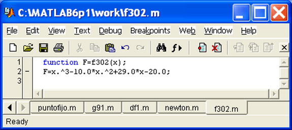
Using Newton’s method calculate the root of the equation x3 – 10x2 + 29x – 20 = 0 close to the point x = 7 with an accuracy of 0.00005. Repeat the same calculation but with an accuracy of 0.0005.
We define the function f(x) =x3 – 10x2 + 29x – 20 and its derivative via the M-files named f302.m and f303.m shown in Figures 8-32 and 8-33.

To run the program that solves the equation, type:
>> [x, it]=newton('f302','f303',7,.00005)
x =
5.0000
it =
6
In 6 iterations and with an accuracy of 0.00005 the solution x = 5 has been obtained. In 5 iterations and with an accuracy of 0.0005 we get the solution x = 5.0002:
>> [x, it] = newton('f302','f303',7,.0005)
x =
5.0002
it =
5
EXERCISE 8-3
Write a program that calculates a root with multiplicity 2 of the equation (e-x -x)2 = 0 close to the point x = -2 to an accuracy of 0.00005.
We define the function f (x)=(ex - x)2 and its derivative via the M-files f304.m and f305.m shown in Figures 8-34 and 8-35:


We solve the equation using Schröder’s method. To run the program we enter the command:
>> [x,it]=schroder('f304','f305',2,-2,.00005)
x =
0.5671
it =
5
In 5 iterations we have found the solution x = 0.56715.
EXERCISE 8-4
Approximate the derivative of the function


To begin we define the function f in the M-file funcion1.m shown in Figure 8-36.

The derivative can be found using the method of numerical derivation with an accuracy of 0.0001 via the following MATLAB command:
>> [L, n] = derivedlim ('funcion1', (1 + sqrt (5)) / 3,0.0001)
L =
1.00000000000000 0.94450896913313 0
0.10000000000000 1.22912035588668 0.28461138675355
0.01000000000000 1.22860294102802 0.00051741485866
0.00100000000000 1.22859747858110 0.00000546244691
0.00010000000000 1.22859742392997 0.00000005465113
n =
4
We see that the value of the derivative is approximated by 1.22859742392997.
Using Richardson’s method, the derivative is calculated as follows:
>> [D, absoluteerror, relativeerror, n] = ('funcion1' richardson,(1+sqrt(5))/3,0.0001,0.0001)
D =
Columns 1 through 4
0.94450896913313 0 0 0
1.22047776163545 1.31246735913623 0 0
1.23085024935646 1.23430774526347 1.22909710433862 0
1.22938849854454 1.22890124827389 1.22854081514126 1.22853198515400
1.22880865382036 1.22861537224563 1.22859631384374 1.22859719477553
Column 5
0
0
0
0
1.22859745049954
absoluteerror =
6. 546534553897310e-005
relativeerror =
5. 328603742973844e-005
n =
5
EXERCISE 8-5
Approximate the following integral:

We can use the composite Simpson’s rule with M=100 using the following command:
>> s = compositesimpson('function1',1,2*pi/3,100)
s =
0.68600990924332
If we use the trapezoidal rule instead, we get the following result:
>> s = trapezoidalrule('function1',1,2*pi/3,100)
s =
0.68600381840334
EXERCISE 8-6
Find an approximate solution of the following differential equation in the interval [0, 0.8]:
![]()
We start by defining the function f(t, y) via the M-file in Figure 8-37.

We then solve the differential equation by Euler’s method, dividing the interval into 20 subintervals using the following command:
>> E = euler('dif2',0,0.8,1,20)
E =
0 1.00000000000000
0.04000000000000 1.04000000000000
0.08000000000000 1.08332800000000
0.12000000000000 1.13052798222336
0.16000000000000 1.18222772296696
0.20000000000000 1.23915821852503
0.24000000000000 1.30217874214655
0.28000000000000 1.37230952120649
0.32000000000000 1.45077485808625
0.36000000000000 1.53906076564045
0.40000000000000 1.63899308725380
0.44000000000000 1.75284502085643
0.48000000000000 1.88348764754208
0.52000000000000 2.03460467627982
0.56000000000000 2.21100532382941
0.60000000000000 2.41909110550949
0.64000000000000 2.66757117657970
0.68000000000000 2.96859261586445
0.72000000000000 3.33959030062305
0.76000000000000 3.80644083566367
0.80000000000000 4.40910450907999
The solution can be graphed as follows (see Figure 8-38):
>> plot (E (:,2))
