CHAPTER 1

Introduction to MATLAB

1.1 Numerical Calculations with MATLAB

You can use MATLAB as a powerful numerical calculator. While most calculators handle numbers only to a preset degree of accuracy, MATLAB works to whichever precision is necessary for any given calculation. In addition, unlike calculators, we can perform operations not only with individual numbers, but also with objects such as matrices.

Most classical numerical analysis topics are treated by MATLAB. It supports matrix algebra, statistics, interpolation, fit by least squares, numerical integration, minimization of functions, linear programming, numerical solutions of algebraic equations and differential equations and a long list of further techniques.

Here are some examples of numerical calculations with MATLAB (once the commands have been entered to the right of the input prompt “>>” simply hit Enter to obtain the result):

1. We can calculate 4 + 3 and get 7 as a result. To do this, just type 4 + 3 and then Enter:

   >> 4 + 3
   
   ans =
   
        7

2. We can also find the value of 3 raised to the power 100, without previously fixing the precision. For this it is enough to simply type 3 ^ 100:

   >> 3 ^ 100
   
   ans =
   
     5. 1538e + 047

3. We can also use the command format long e to obtain results in scientific notation with 16 more exponential digits of precision:

   >> format long e;
   >> 3 ^ 100
   
   ans =
   
       5.153775207320115e+047

4. We can also work with complex numbers. We find the result of the operation raising (2 + 3i) to the power 10 by typing the expression (2 + 3i) ^ 10:

   >> (2 + 3i) ^ 10
   
   ans =
   
       -3 415250000000001e + 005 - 1. 456680000000001e + 005i

   The command format long g will optimize the output of future calculations.

   >> format long g
   >> (2 + 3i) ^ 10
   
   ans =
   
        -341525 - 145668i

5. The previous result can also be obtained in short format using the command format short:

   >> format short;
   >> (2 + 3i) ^ 10
   
   ans =
   
       -3.4152e+005- 1.4567e+005i

6. We can calculate the value of the Bessel function at the point 13.5. To do this, we type Besselj(0,13.5):

   >> Besselj(0,13.5)
   
   ans =
   
       0.2150

7. We can also perform numerical integration. To calculate the integral between 0 and π of sin(x), we type the expression int(sin(x), 0, pi) after having declared the variable x as symbolic with the command syms:

   >> syms x
   >> int(sin(x), 0, pi)
   
   ans =
   
   2

These themes will be treated more thoroughly later.

1.2 Symbolic Calculations with MATLAB

MATLAB handles symbolic mathematical computation perfectly, manipulating formulae and algebraic expressions easily and efficiently. You can expand, factor and simplify polynomials, rational functions and trigonometric expressions; you can find algebraic solutions of polynomial equations and systems of equations; you can evaluate derivatives and integrals symbolically and find solutions of differential equations; you can manipulate power series, find limits and explore many other facets of algebraic series.

To perform this task, MATLAB requires that all variables (or algebraic expressions) are previously declared as symbolic using the command syms.

Here are some examples of symbolic computations with MATLAB:

1. We find the cube of the algebraic expression: (x + 1)(x + 2) - (x + 2)^2. This is done by typing the expression: expand((x + 1)*(x + 2) - (x + 2)^2)^3). The result will be another algebraic expression:

   >> syms x
   >> expand (((x + 1)*(x + 2)-(x + 2)^2)^3).
   
   ans =
   
   -x ^ 3-6 * x ^ 2-12 * x-8

2. We can factor the result of the above calculation by typing factor((x + 1) *(x + 2) - (x + 2)^2)^3):

   >> syms x
   >> factor(((x + 1)*(x + 2)-(x + 2)^2)^3)
   
   ans =
   
   -(x+2) ^ 3

3. We can find the indefinite integral of the function
   (x ^ 2)sin(x)^2 by typing int(x^2 * sin(x)^2, x):

   >> syms x
   >> int(x^2*sin(x)^2, x)
   
   ans =
   
   x ^ 2 * (-1/2 * cos(x) * sin(x) + 1/2 * x)-1/2 * x * cos(x) ^ 2 + 1/4 * cos(x) * sin(x) + 1/4 * 1/x-3 * x ^ 3

4. We can simplify the previous result:

   >> syms x
   >> simplify(int(x^2*sin(x)^2, x))
   
   ans =
   
   -1/2 * x ^ 2 * cos(x) * sin(x) + 1/6 * x ^ 3-1/2 * x * cos(x) ^ 2 + 1/4 * cos(x) * sin(x) + 1/4 * x

5. We can display the previous result in standard mathematical notation:

   >> syms x
   >> pretty(simplify(int('x^2*sin(x)^2', 'x')))
   
                2              3              2
   -1/2 x cos(x) sin(x) + 1/6 x - 1/2 x cos(x) + 1/4 cos(x) sin(x) + 1/4 x

6. We can expand the function x^2 * sin(x)^2 as a power series up to order 12, presenting the result in standard form:

   >> syms x
   >> pretty(taylor(x^2*sin(x)^2,12))
   
   
       4     6       8         10      12
     x 1/3 x + 2/45 x - 1/315 x + 0 (x)

7. We can solve the equation 3ax 7x^2 + x^3 = 0 (where a is a parameter):

   >> syms x a
   >> solve('3*a*x-7*x^2 + x^3 = 0', x)
   
   ans =
   
   [         0                  ]
   [7/2 + 1/2 *(49-12*a) ^(1/2)]
   [7/2-1/2 *(49-12*a) ^(1/2)  ]
   

8. We can find the five solutions of the equation x^5 + 2x + 1 = 0 :

   >> syms x
   >> solve('x^5+2*x+1','x')
   
   ans =
   
   [-.7018735688558619 -.8796971979298240 * i]
   [-.7018735688558619 +.8796971979298240 * i]
   [-.4863890359345430                       ]
   [ .9450680868231334 -.8545175144390459 * i]
   [ .9450680868231334 +.8545175144390459 * i]

On the other hand, MATLAB can be used together with the Maple program libraries to work with symbolic mathematics, thus extending its field of action. In this way, MATLAB can be used to work on topics such as differential forms, Euclidean geometry, projective geometry, statistics, etc.

At the same time, we can extend MATLAB’s numerical calculation cababilities by using the Maple libraries (combinatorics, optimization, number theory, statistics, etc.)

1.3 MATLAB and Maple

Whenever it is necessary to use a Maple command or function from MATLAB, use the command maple followed by the corresponding Maple syntax. This functionality is only available if you have installed the symbolic computation Toolbox “Extended Symbolic Math Toolbox”. This is the tool one uses to work with linear algebra and mathematical analysis.

To use a Maple command from MATLAB, the syntax is as follows:

• maple(‘Maple_command_syntax’)
• or alternatively:
• maple ‘Maple_command_syntax’
• To use a Maple command with N arguments from MATLAB, the syntax is as follows:
• maple(‘Maple_command_syntax’, argument1, argument2, . . . , argumentN)

Let’s see some examples:

1. We can calculate the limit of the function (x^3 -1) / (x-1) as x - > 1:

   >> maple('limit((x^3-1)/(x-1),x=1)')
   
   ans =
   
   3

   We could also have used the following syntax:

   >> maple 'limit((x^3-1)/(x-1),x=1)'
   
   ans =
   
   3

2. We can calculate the greatest common divisor of 10,000 and 5,000:

   >> maple('gcd', 10000, 5000)
   
   ans =
   
   5000

1.4 General Notation. The Command Window

Whenever a program is used, it is necessary to become familiar with the general characteristics of its notation. Like any program, the best way to learn MATLAB is to use it. Each example consists of the user input prompt “>>” followed by the command and the MATLAB response on the next line. See Figure 1-1.

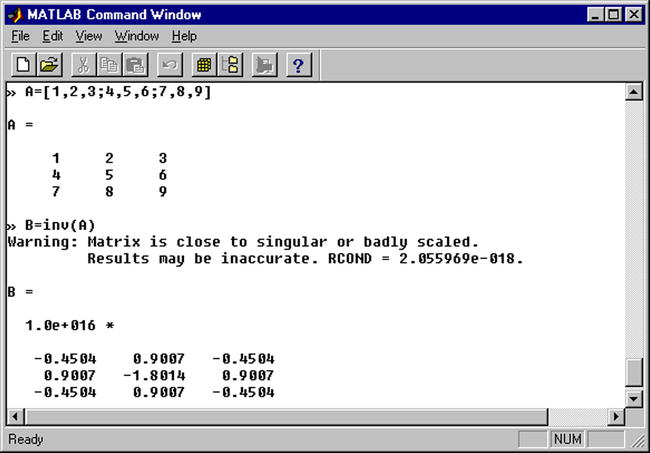
Sometimes, depending on the type of command (user input) given to MATLAB in the Command Window, the response will begin with the expression ans =. See Figure 1-2.

It is important to pay attention to uppercase and lowercase characters, parentheses and square brackets, and the use of spaces and punctuation (in particular commas and semicolons).

Like the C programming language, MATLAB is case sensitive; for example, Sin(x) is different to sin(x). The names of all built-in functions begin with lowercase letters. Each bracket has its own meaning, as we will see later.

To indicate that two variables must be multiplied you put the symbol * between them, and there cannot be spaces in the names of commands, variables or functions. In other cases, spaces are ignored, but they can be included to make the input more readable.

Once a MATLAB command has been entered, simply press Enter. If at the end of the input we put a semicolon, the program runs the calculation and keeps it in memory (Workspace), but does not display the result on screen. The input prompt “>>” reappears to indicate that you can input a new entry.

>> 2 + 3;
>>

If the entry is too long and doesn’t fit on a single line of the MATLAB Command Window, just put three dots at the end of the line and press Enter to continue with the rest of the entry on the next line. Once the entry is complete, press Enter to run the command:

>> 1254 + 3456789 + 14267890 + 345217 +...
78965 + 125347 + 86500

ans =

    18361962
>>

You can make multiple entries in the same command line by separating them with commas and pressing Enter at the end of the last entry. If you use a semicolon at the end of one of the entries of the line, its corresponding output is ignored. If the number of consecutive entries doesn’t fit on one line, three dots are used to continue on the next line, as described above:

>> 2+2, 5+3, 8+5

ans =

     4

ans =

     8

ans =

    13

>> 2+2; 5+3, 8+5; 3*4

ans =

     8

ans =

    12

To enter a descriptive comment in a command line, just start it with the “%” symbol. When you run the input, MATLAB will ignore the comment and process the rest.

>> F = 125 + 2 %F represents units of force

F =

   127

To simplify the process of entering a script to be evaluated by the MATLAB interpreter (via the command window prompt), you can use arrow keys. For example, if you press the up arrow once, you recover the last entry submitted in MATLAB. If you press the up arrow twice, you recover the penultimate entry submitted, and so on.

If you type a sequence of characters in the input area and then click the up arrow, you recover the last entry that begins with the specified string.

The commands entered during a MATLAB session are stored temporarily in the buffer (Workspace) until the end of the session, at which time you can permanently save the session to file or lose it.

Below is a summary of the keys that can be used in the MATLAB command line, and their functions:

The command clc clears the command window, but does not delete the contents of the work area (the content currently in memory).

1.5 MATLAB and Programming

By properly combining all the features of MATLAB, one can build useful mathematical research programming code. Programs usually consist of a sequence of instructions in which various values are calculated. These sequences of commands are assigned names and can be reused in further calculations.

As in programming languages like C or Fortran, MATLAB supports loops, control flow and conditional statements. MATLAB can write procedural programs, i.e., it can define a sequence of standard steps to run. As in C or Pascal, one can repeat calculations using Do, For, or While loops. The language of MATLAB also includes conditional constructs such as If Then Else. MATLAB also supports different logical operators, such as And, Or, Not and Xor.

MATLAB supports procedural programming (with iterative processes, recursive functions, loops...), functional programming and object-oriented programming. Here are two simple examples of programs. The first generates the order n Hilbert matrix, and the second calculates the Fibonacci numbers less than 1000.

% Generates the order n Hilbert matrix
t = '1/(i+j-1)';
for i = 1:n
      for j = 1:n
           a(i,j) = eval(t);
      end
 end

% Calculates Fibonacci numbers
f = [1 1]; i = 1;
while f(i) + f(i-1) < 1000
          f(i+2) = f(i) + f(i+1);
          i = i+1
end

1.6 Translating C, FORTRAN and TEX expressions

MATLAB offers the possibility to translate math expressions to code in other programming languages such as Fortran or C. Additionally, it can also translate expressions to eqn and TeX form. To do this, one can use the following commands:

• maple(‘fortran(expression)’) Translates the given Maple expression to Fortran.
• maple(‘fortran(expr,optimized)’) Translates the given Maple expression to Fortran in an optimized way.
• maple(‘fortran(expr,precision=double)’) Translates the Maple expression to Fortran using double-precision.
• maple(‘fortran(expr,digits=n)’) Translates the Maple expression to Fortran using n floating point digits.
• maple(‘fortran(procedure)’) Translates the given Maple procedure to a Fortran procedure. Also translates Maple arrays and lists to Fortran.
• maple(‘fortran(exp,filename=name)’) Translates the given Maple expression to Fortran and saves it in a file named name.
• maple(‘C(expression)’) Translates the given Maple expression to C. It is necessary to first load the C library with the command readlib(C).
• maple(‘C(expression,optimized)’) Translates the given Maple expression into C in an optimized way.
• maple(‘C(expr,precision=single)’) Translates the given Maple expression into C using single-precision (double precision is the default).
• maple(‘C(expr,digits=n)’) Translates the given Maple expression into C using n floating point digits.
• maple(‘C(procedure)’) Translates the given Maple procedure to a C procedure. It also translates Maple arrays and lists to C.
• maple(‘C(procedure, ansi)’) Translates the given Maple procedure to C following standard ANSI C syntax for the declaration of the parameters.
• maple(‘C(expr, filename=name)’) Translates the given Maple expression to C and saves it in a file with the name nom.
• maple(‘latex(expression)’) Converts the given Maple expression to TeX.
• maple(‘latex(expr, filename=name)’) Converts the given Maple expression to TeX and saves it in a file named nom.
• maple(‘eqn(expression)’) Translates the given Maple expression to eqn. It is necessary to first load the eqn library with the command readlib(eqn).
• maple(‘eqn(expr, filename=name)’) Translates the given Maple expression to eqn and saves it in a file with the name name.

As examples, we translate the integral of 1 /(x⁴+1) to TeX, Fortan and C:

>> maple('latex(Int(1/(x^4+1),x))')

ans =

    int !left ({x}^{4}+1
ight )^{-1}{dx}

>> maple('fortran(Int(1/(x^4+1),x))')

ans =

     t0 = Int(1/(x**4+1),x)

>> maple('readlib(C)'); maple('C(Int(1/(x^4+1),x))')

ans =

     t0 = Int(1/(pow(x,4.0)+1.0),x);