![]()
Building Churn Models
In this chapter, we reveal the secrets of building customer churn models, which are in very high demand. Many industries use churn analysis as a means of reducing customer attrition. This chapter will show a holistic view of building customer churn models in Microsoft Azure Machine Learning.
Churn Models in a Nutshell
Businesses need to have an effective strategy for managing customer churn because it costs more to attract new customers than to retain existing ones. Customer churn can take different forms, such as switching to a competitor’s service, reducing the time spent using the service, reducing the number of services used, or switching to a lower-cost service. Companies in the retail, media, telecommunication, and banking industries use churn modeling to create better products, services, and experiences that lead to a higher customer retention rate.
Let’s drill deeper into why churn modeling matters to telecommunication companies. The consumer business of many telecommunication companies operates in an immensely competitive market. In many countries, it is common to have two or more telecommunication companies competing for the same customer. In addition, mobile number portability makes it easier for customers to switch to another telecommunication provider.
Many telecommunication companies track churn levels as part of their annual report. The use of churn models has enabled telecommunication providers to formulate effective business strategies for customer retention, and to prevent potential revenue loss.
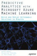
Churn models enable companies to predict which customers are most likely to churn, and to understand the factors that cause churn to occur. Among the different machine learning techniques used to build churn models, classification algorithms are commonly used. Azure Machine Learning provides a wide range of classification algorithms including decision forest, decision jungle, logistic regression, neural networks, Bayes point machines, and support vector machines. Figure 6-1 shows the different classification algorithms that you can use in Azure Machine Learning Studio.
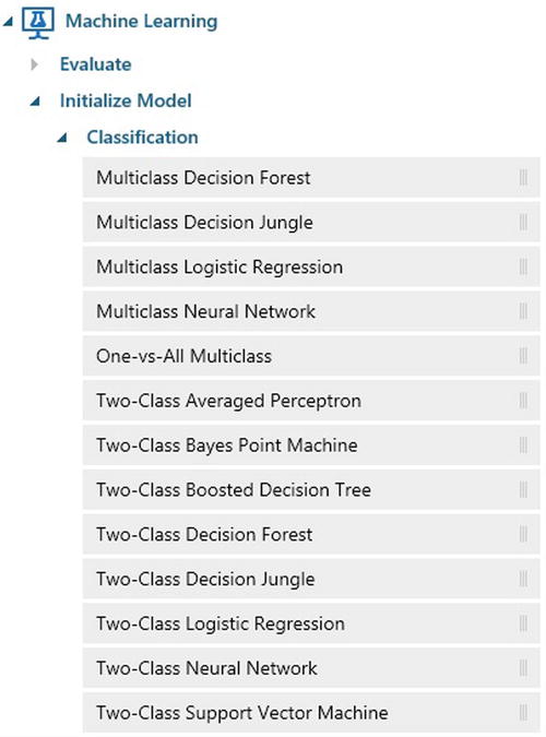
Figure 6-1. Classification algorithms available in ML Studio
Prior to building the churn model (based on classification algorithms), understanding the data is very important. Given a dataset that you are using for both training and testing the churn model, you should ask the following questions (non-exhaustive) about the data:
- What kind of information is captured in each column?
- Should you use the information in each column directly, or should you compute derived values from each column that are more meaningful?
- What is the data distribution?
- Are the values in each column numeric or categorical?
- Does a column consists of many missing values?
Once you understand the data, you can start building the churn model using the following steps.
- Data preparation and understanding
- Data preprocessing and feature selection
- Classification model for predicting customer churn
- Evaluating the performance of the model
- Operationalizing the model
In this chapter, you will learn how to perform each of these steps to build a churn model for a telecommunication use case. You will learn the different tools that are available in Azure Machine Learning Studio for understanding the data and performing data preprocessing. And you will learn the different performance metrics that are used for evaluating the effectiveness of the model. Let’s get started!
Building and Deploying a Customer Churn Model
In this section, you will learn how to build a customer churn model using different classification algorithms. For building the customer churn model, you will be using a telecommunication dataset from KDD Cup 2009. The dataset is provided by a leading French telecommunication company, Orange. Based on the Orange 2013 Annual Report, Orange has 236 million customers globally (15.5 million fixed broadband customers and 178.5 million mobile customers).
The goal of the KDD Cup 2009 challenge is to build an effective machine learning model for predicting customer churn, willingness to buy new products/services (appetency), and opportunities for up-selling. In this section, you will focus on predicting customer churn.
![]() Note KDD Cup is an annual competition organized by the ACM Special Interest Group on Knowledge Discovery and Data Mining (SIGKDD). Each year, data scientists participate in various data mining and knowledge discovery challenges. These challenges range from predicting who is most likely to donate to a charity (1997), clickstream analysis for an online retailer (2000), predicting movie rating behavior (2007), to predicting the propensity of customers to switch providers (2009).
Note KDD Cup is an annual competition organized by the ACM Special Interest Group on Knowledge Discovery and Data Mining (SIGKDD). Each year, data scientists participate in various data mining and knowledge discovery challenges. These challenges range from predicting who is most likely to donate to a charity (1997), clickstream analysis for an online retailer (2000), predicting movie rating behavior (2007), to predicting the propensity of customers to switch providers (2009).
Preparing and Understanding Data
In this exercise, you will use the small Orange dataset, which consists of 50,000 rows. Each row has 230 columns (referred to as variables). The first 190 variables are numerical and the last 40 variables are categorical.
Before you start building the experiment, download the following small dataset and the churn labels from the KDD Cup web site:
- orange_small_train.data.zip - www.sigkdd.org/site/2009/files/orange_small_train.data.zip
- orange_small_train_churn.labels - www.sigkdd.org/site/2009/files/orange_small_train_churn.labels
In the orange_small_train_churn.labels file, each line consists of a +1 or -1 value. The +1 value refers to a positive example (the customer churned), and the -1 value refers to a negative example (the customer did not churn).
Once the file has been uploaded, you should upload the dataset and the labels to Machine Learning Studio, as follows:
- Click New and choose Dataset
 From Local File (Figure 6-2).

Figure 6-2. Uploading the Orange dataset using Machine Learning Studio
- Next, choose the file to upload: orange_small_train.data (Figure 6-3) .
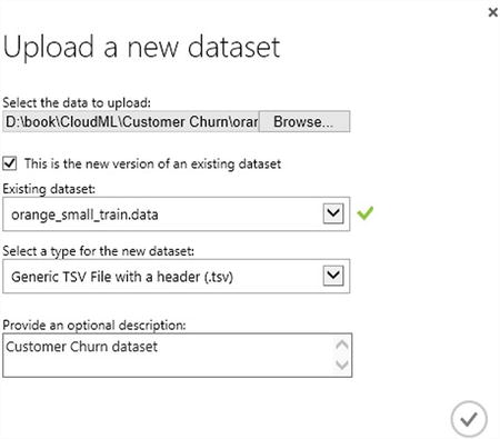
Figure 6-3. Uploading the dataset
- Click OK.
After the Orange dataset has been uploaded, repeat the steps to upload the churn labels file to Machine Learning Studio. Once this is done, you should be able to see the two Orange datasets when you create a new experiment. To do this, create a new experiment, and expand the Saved Datasets menu in the left pane. Figure 6-4 shows the Orange training and churn labels datasets that you uploaded.
Figure 6-4. Saved Datasets, Orange Training Data and Churn Labels
When building any machine learning model, it is very important to understand the data before trying to build the model. To do this, create a new experiment as follows.
- Click New Experiment.
- Name the experiment - Understanding the Orange Dataset.
- From Saved Datasets, choose the orange_small_train.data dataset (double-click it).
- From Statistical Functions, choose Descriptive Statistics (double-click it).
- You will see both modules. Connect the dataset with the Descriptive Statistics module. Figure 6-5 shows the completed experiment.
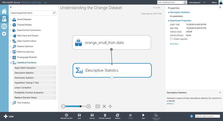
Figure 6-5. Understanding the Orange dataset
- Click Run.
- Once the run completes successfully, right-click the circle below Descriptive Statistics and choose Visualize.
- You will see an analysis of the data, which covers Unique Value Count, Missing Value Count, Min, and Max for each of the variables (Figure 6-6).
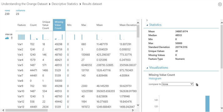
Figure 6-6. Descriptive statistics for the Orange dataset
This provides useful information on each of the variables. From the visualization, you will observe that there are lots of variables with missing values (e.g., Var1, Var8). For example, Var8 is practically a column with no useful information.
![]() Tip When visualizing the output of Descriptive Statistics, it shows the top 100 variables. To see all the statistics for all the 230 variables, right-click the bottom circle of Descriptive Statistic module and choose Save as dataset. After the dataset has been saved, you can choose to download the file and see all the rows in Excel.
Tip When visualizing the output of Descriptive Statistics, it shows the top 100 variables. To see all the statistics for all the 230 variables, right-click the bottom circle of Descriptive Statistic module and choose Save as dataset. After the dataset has been saved, you can choose to download the file and see all the rows in Excel.
Data Preprocessing and Feature Selection
In most classification tasks, you will often have to identify which of the variables should be used to build the model. Machine Learning Studio provides two feature selection modules that can be used to determine the right variables for modeling. This includes filter-based feature selection and linear discriminant analysis.
For this exercise, you will not be using these feature selection modules. Figure 6-7 shows the data preprocessing steps.
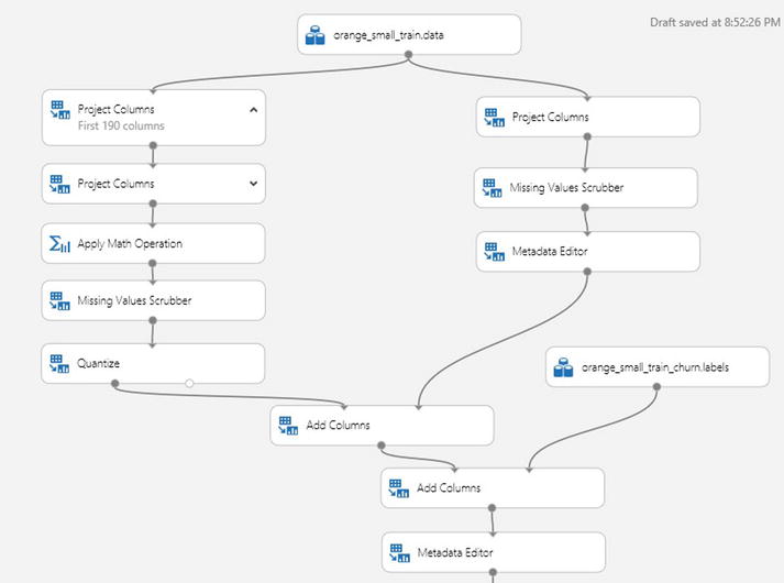
Figure 6-7. Data preprocessing steps
For simplicity, perform the following steps to preprocess the data.
- Divide the variables into the first 190 columns (numerical data) and the remaining 40 columns (categorical data). To do this, add two Project Columns modules.
For the first Project Column module, select Column indices: 1-190 (Figure 6-8).
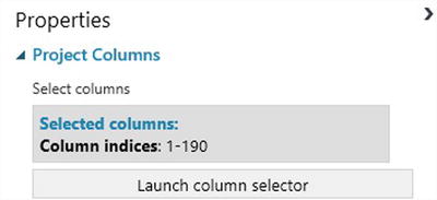
Figure 6-8. Selecting column indices 1-190 (numerical columns)
For the second Project Column module, select Column indices: 191-230 (Figure 6-9).
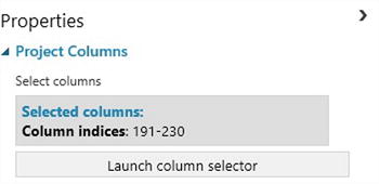
Figure 6-9. Selecting column indices 191-230 (categorical columns)
- For the first 190 columns, do the following:
- Use Project Columns to select the columns that contain numerical data (and remove columns that contain zero or very few values). These includes the following columns: Var6, Var8, Var15, Var20, Var31, Var32, Var39, Var42, Var48, Var52, Var55, Var79, Var141, Var167, Var175, and Var185. Figure 6-10 shows the columns that are excluded.
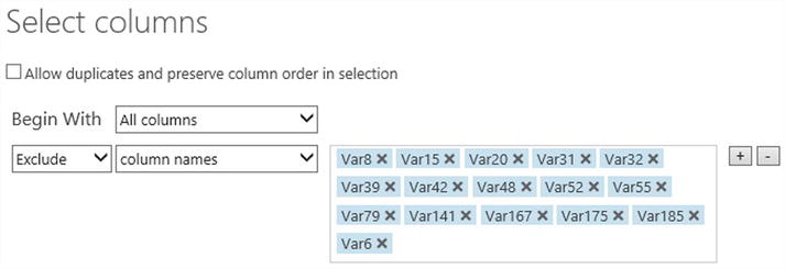
Figure 6-10. Excluding columns that do not contain useful values
- Apply a math operation that adds 1 to each row. The rationale is that this enables you to distinguish between rows that contain actual 0 for the column vs. the substitution value 0 (when you use the Missing Values Scrubber). Figure 6-11 shows the properties for the Math Operation module.
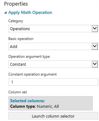
Figure 6-11. Adding 1 to existing numeric variables
- Use the Missing Value Scrubber to substitute missing values with 0. Figure 6-12 shows the properties.
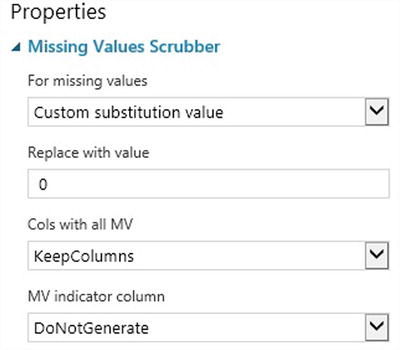
Figure 6-12. Missing Values Scrubber properties
- Use the Quantize module to map the input values to a smaller number of bins using a quantization function. In this exercise, you will use the EqualWidth binning mode. Figure 6-13 shows the properties used.
- Use Project Columns to select the columns that contain numerical data (and remove columns that contain zero or very few values). These includes the following columns: Var6, Var8, Var15, Var20, Var31, Var32, Var39, Var42, Var48, Var52, Var55, Var79, Var141, Var167, Var175, and Var185. Figure 6-10 shows the columns that are excluded.
- For the remaining 40 columns, perform the following steps:
- Use the Missing Values Scrubber to substitute it with 0. Figure 6-14 shows the properties.
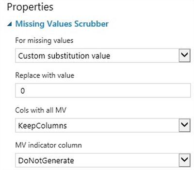
Figure 6-14. Missing Values Scrubber (for the remaining 40 columns)
- Use the Metadata Editor to change the type for all columns to be categorical. Figure 6-15 shows the properties.
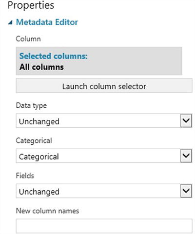
Figure 6-15. Using the Metadata Editor to mark the columns as containing categorical data
- Use the Missing Values Scrubber to substitute it with 0. Figure 6-14 shows the properties.
- Combine it with the labels from the ChurnLabel dataset. Figure 6-16 shows the combined data.
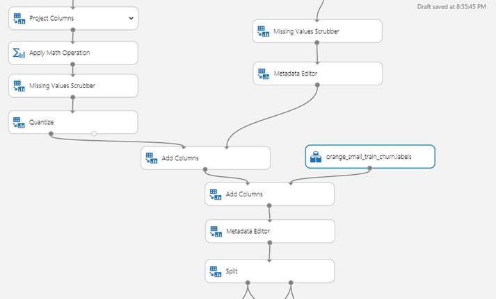
Figure 6-16. Combining training data and training label
- Rename the label column as ChurnLabel. Figure 6-17 shows how you can use the Metadata Editor to rename the column.
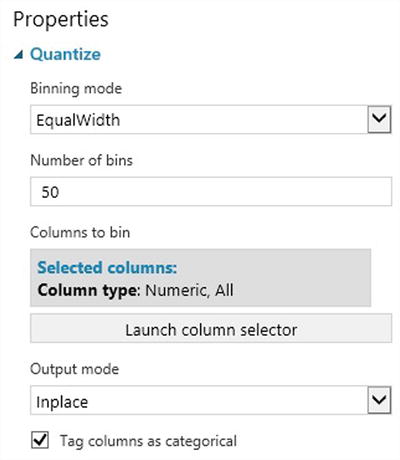
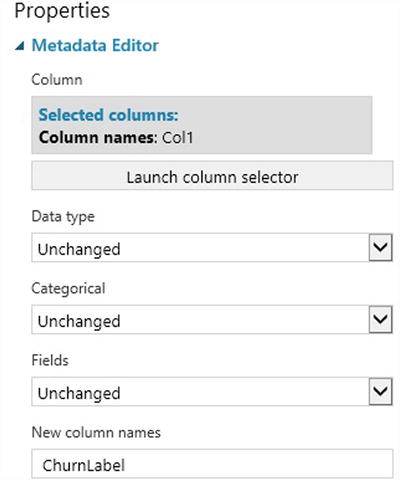
Figure 6-17. Renaming the label column as ChurnLabel
Classification Model for Predicting Churn
In this section, you will start building the customer churn model using the classification algorithms provided in Azure Machine Learning Studio. For predicting customer churn, you will use two classification algorithms, a two-class boosted decision tree and a two-class decision forest.
A decision tree is a machine learning algorithm for classification or regression. During training, it splits the data using the input variables that give the highest information gain. The process is repeated on each subset of the data until splitting is no longer required. The leaf of the decision tree identifies the label to be predicted (or class). This prediction is provided based on a probability distribution.
The boosted decision tree and decision forest algorithms build an ensemble of decision trees and use them for predictions. The key difference between the two approaches is that, in boosted decision tree algorithms, multiple decision trees are grown in series such that the output of one tree is provided as input to the next tree. This is a boosting approach to ensemble modeling. In contrast, the decision forest algorithm grows each decision tree independently of each other; each tree in the ensemble uses a sample of data drawn from the original dataset. This is the bagging approach of ensemble modeling. See Chapter 4 for more details on decision trees, decision forests, and boosted decision trees. Figure 6-18 shows how the data is split and used as inputs to train the two classification models.
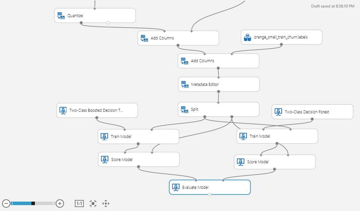
Figure 6-18. Splitting the data into training and testing, and training the customer churn model
From Figure 6-18, you can see that the following steps are performed.
- Splitting the input data into training and test data: In this exercise, you split the data by specifying the Fraction of rows in the first output dataset, and set it as 0.7. This assigns 70% of data to the training set and the remaining 30% to the test dataset.
Figure 6-19 shows the properties for Split.
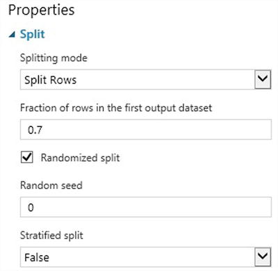
Figure 6-19. Properties of the Split module
- Training the model using the training data: In this exercise, you will be training two classification models, a two-class boosted decision tree and two-class decision forest. Figures 6-20 and 6-21 show the properties for each of the classification algorithms.
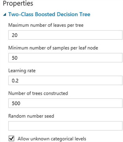
Figure 6-20. Properties for two-class boosted decision tree
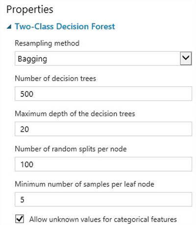
Figure 6-21. Properties for two-class decision forest
- Training the model using the Train Model module: To train the model, you need to select the label column. In this exercise, you will be using the ChurnLabel column. Figure 6-22 shows the properties for Train Model.
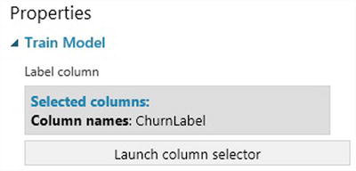
Figure 6-22. Using ChurnLabel as the Label column
Scoring the model: After training the customer churn model, you can use the Score Model module to predict the label column for a test dataset. The output of Score Model will be used in Evaluate Model to understand the performance of the model.
Congratulations, you have successfully built a customer churn model! You learned how to use two of the classification algorithms available in Machine Learning Studio. You also learned how to evaluate the performance of the model. In the next few chapters, you will learn how to deploy the model to production and operationalize it.
Evaluating the Performance of the Customer Churn Models
After you use the Score Model to predict whether a customer will churn, the output of the Score Model module is passed to the Evaluate Model to generate evaluation metrics for each of the model. Figure 6-23 shows the Score Model and Evaluate Model modules.
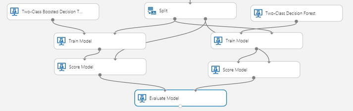
Figure 6-23. Scoring and evaluating the model
After you have evaluated the model, you can right-click the circle at the bottom of Evaluate Model to see the performance of the two customer churn models. Figure 6-24 shows the Receiver Operating Characteristic (ROC curve) while Figure 6-25 shows the accuracy, precision, recall, and F1 scores for the two customer churn models.
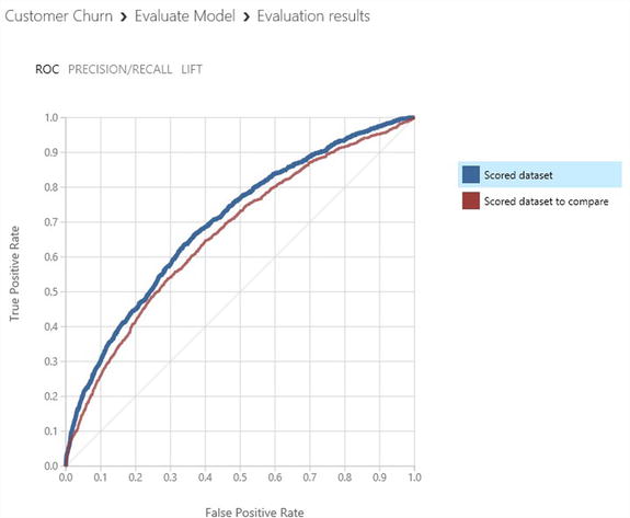
Figure 6-24. ROC curve for the two customer churn models
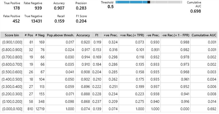
Figure 6-25. Accuracy, precision, recall, and F1 scores for the customer churn models
The ROC curve shows the performance of the customer churn models. The diagonal line from (0,0) to (1,1) on the chart shows the performance of random guessing. For example, if you randomly guessed which customer would churn, the curve will be on the diagonal line. A good predictive model should perform better than random guessing, and the ROC curve should be above the diagonal line. The performance of a customer churn model can be measured by considering the area under the curve (AUC). The higher the area under the curve, the better the model’s performance. The ideal model will have an AUC of 1.0, while a random guess will have an AUC of 0.5.
From the visualization, you can see that the customer churn models have a cumulative AUC, accuracy, and precision of 0.698, 0.907, and 0.283, respectively. You can also see that the customer models have a F1 score of 0.204.
![]() Note See http://en.wikipedia.org/wiki/F1_score for a good discussion on the use of the F1 score to measure the accuracy of the machine learning model.
Note See http://en.wikipedia.org/wiki/F1_score for a good discussion on the use of the F1 score to measure the accuracy of the machine learning model.
Summary
Using the KDD Cup 2009 Orange telecommunication dataset, you learned step by step how to build customer churn models using Azure Machine Learning. Before building the model, you took time to first understand the data and perform data preprocessing. Next, you learned how to use the two-class boosted decision tree and two-class decision forest algorithms to perform classification, and to build a model for predicting customer churn with the telecommunication dataset. After building the model, you also learned how to measure the performance of the models.