
![]()
The Fundamentals
Success is neither magical nor mysterious. Success is the natural consequence of consistently applying the basic fundamentals.
—Jim Rohn, American entrepreneur and motivational speaker
I have a love–hate relationship with fundamentals. The easier the task seems to be, the less enjoyable I seem to find it, at least unless I already have a love for the topic at some level. In elementary school, there were fun classes, like recess and lunch for example. But when handwriting class came around, very few kids really liked it, and most of those who did just loved the taste of the pencil lead. But handwriting class was an important part of childhood educational development. Without it, you wouldn’t be able to write on a white board, and without that skill, could you actually stay employed as a programmer? I know I personally am addicted to the smell of whiteboard marker, which might explain more than my vocation.
Much like handwriting was an essential skill for life, database design has its own set of skills that you need to get under your belt. While database design is not a hard skill to learn, it is not exactly a completely obvious one either. In many ways, the fact that it isn’t a hard skill makes it difficult to master. Databases are being designed all of the time by people of limited understanding of what makes one “good.” Administrative assistants build databases using Excel, kids make inventories of their video games on a sheet of paper, and newbie programmers build databases with all sorts of database management tools, and rarely are any of the designs and implementations 100% wrong. The problem is that in almost every case the design produced is fundamentally flawed, causing future modifications to be very painful. When you are finished with this book, you should be able to design databases that reduce the effects of many of the common fundamental blunders. If a journey of a million miles starts with a single step, the first step in the process of designing quality databases is understanding why databases are designed the way they are, and this requires us to cover the fundamentals.
I know this topic may bore you, but would you drive on a bridge designed by an engineer who did not understand physics? Or would you get on a plane designed by someone who didn’t understand the fundamentals of flight? Sounds quite absurd, right? So, would you want to store your important data in a database designed by someone who didn’t understand the basics of database design?
The first five chapters of this book are devoted to the fundamental tasks of relational database design and preparing your mind for the task at hand: implementing a relational database. The topics won’t be particularly difficult in nature, and I will do my best to keep the discussion at the layman’s level, and not delve so deeply that you punch me if you pass me in the hall at the PASS Summit (www.sqlpass.org).
For this chapter, we will start out looking at basic background topics that are very useful.
- History: Where did all of this relational database stuff come from? In this section I will present some history, largely based on Codd’s 12 Rules as an explanation for why the RDBMS (Relational Database Management System) is what it is.
- Relational data structures: This section will provide introductions of some of the fundamental database objects, including the database itself, as well as tables, columns, and keys. These objects are likely familiar to you, but there are some common misunderstandings in their usage that can make the difference between a mediocre design and a high-class, professional one.
- Relationships between entities: We will briefly survey the different types of relationships that can exist between the relational data structures introduced in the relational data structures section.
- Dependencies: The concept of dependencies between values and how they shape the process of designing databases later in the book will be discussed.
- Relational programming: This section will cover the differences between procedural programming using C# or VB (Visual Basic) and relational programming using SQL (Structured Query Language).
- Database design phases: This section provides an overview of the major phases of relational database design: conceptual/logical, physical, and storage. For time and budgetary reasons, you might be tempted to skip the first database design phase and move straight to the physical implementation phase. However, skipping any or all of these phases can lead to an incomplete or incorrect design, as well as one that does not support high-performance querying and reporting.
At a minimum, this chapter on fundamentals should get us to a place where we have a set of common terms and concepts to use throughout this book when discussing and describing relational databases. Throughout my years of reading and research, I’ve noticed that lack of agreed-upon terminology is one of the biggest issues in the database community. Academics have one (well, ten) set(s) of terms to mean the same thing as we people who actually develop code. Sometimes multiple different words are used to mean one concept, but worst case, one word means multiple things. Tradespeople (like myself, and probably you the reader) have their own terminology, and it is usually used very sloppily. I am not immune to sloppy terminology myself when chatting about databases, but in this book I do my best to stick to a single set of terms. Some might say that this is all semantics, and semantics aren’t worth arguing about, but honestly, they are the only thing worth arguing about. Agreeing to disagree is fine if two parties understand one another, but the true problems in life tend to arise when people are in complete agreement about an idea but disagree on the terms used to describe it.
Taking a Brief Jaunt Through History
No matter what country you hail from, there is, no doubt, a point in history when your nation began. In the United States, that beginning came with the Declaration of Independence, followed by the Constitution of the United States (and the ten amendments known as the Bill of Rights). These documents are deeply ingrained in the experience of any good citizen of the United States. Similarly, we have three documents that are largely considered the start of relational databases.
In 1979, Edgar F. Codd, who worked for the IBM Research Laboratory at the time, wrote a paper entitled “A Relational Model of Data for Large Shared Data Banks,” which was printed in Communications of the ACM (“ACM” is the Association for Computing Machinery [www.acm.org]). In this 11-page paper, Codd introduces a revolutionary idea for how to break the physical barriers of the types of databases in use at that time. Then, most database systems were very structure oriented, requiring a lot of knowledge of how the data was organized in the storage. For example, to use indexes in the database, specific choices would be made, like only indexing one key, or if multiple indexes existed, the user was required to know the name of the index to use it in a query.
As most any programmer knows, one of the fundamental tenets of good programming is to attempt low coupling of computer subsystems, and needing to know about the internal structure of the data storage was obviously counterproductive. If you wanted to change or drop an index, the software and queries that used the database would also need to be changed. The first half of Codd’s relational model paper introduced a set of constructs that would be the basis of what we know as a relational database. Concepts such as tables, columns, keys (primary and candidate), indexes, and even an early form of normalization are included. The second half of the paper introduced set-based logic, including joins. This paper was pretty much the database declaration of storage independence.
Moving six years in the future, after companies began to implement supposed relational database systems, Codd wrote a two-part article published by Computerworld magazine entitled “Is Your DBMS Really Relational?” and “Does Your DBMS Run By the Rules?” on October 14 and October 21, 1985. Though it is nearly impossible to get a copy of these original articles, many web sites outline these rules, and I will too. These rules go beyond relational theory and define specific criteria that need to be met in an RDBMS, if it’s to be truly considered relational.
Introducing Codd’s Rules for an RDBMS
I feel it is useful to start with Codd’s rules, because while these rules are over 30 years old, they do probably the best job of setting up not only the criteria that can be used to measure how relational a database is but also the reasons why relational databases are implemented as they are. The neat thing about these rules is that they are seemingly just a formalized statement of the KISS manifesto for database users—keep it simple stupid, or keep it standard, either one. By establishing a formal set of rules and principles for database vendors, users could access data that not only was simplified from earlier data platforms but worked pretty much the same on any product that claimed to be relational. Of course, things are definitely not perfect in the world, and these are not the final principles to attempt to get everyone on the same page. Every database vendor has a different version of a relational engine, and while the basics are the same, there are wild variations in how they are structured and used. The basics are the same, and for the most part the SQL language implementations are very similar (I will discuss very briefly the standards for SQL in the next section). The primary reason that these rules are so important for the person just getting started with design is that they elucidate why SQL Server and other relational engine–based database systems work the way they do.
Rule 1: The Information Principle
All information in the relational database is represented in exactly one and only one way—by values in tables.
While this rule might seem obvious after just a little bit of experience with relational databases, it really isn’t. Designers of database systems could have used global variables to hold data or file locations or come up with any sort of data structure that they wanted. Codd’s first rule set the goal that users didn’t have to think about where to go to get data. One data structure—the table—followed a common pattern of rows and columns of data that users worked with.
Many different data structures were in use in the early days that required a lot of internal knowledge of data. Think about all of the different data structures and tools you have used. Data could be stored in files, a hierarchy (like the file system), or any method that someone dreamed of. Even worse, think of all of the computer programs you have used; how many of them followed a common enough standard that they worked just like everyone else’s? Very few, and new innovations are coming every day.
While innovation is rarely a bad thing, innovation in relational databases is largely limited to the layer that is encapsulated from the user’s view. The same database code that worked 20 years ago could easily work today with the simple difference that it now runs a great deal faster. There have been great advances in the language we use (SQL), but other than a few wonky bits of syntax that have been deprecated (the most common example being *= for left join, and =* for right [no *=* for full outer join]), SQL written 20 years ago will work today, largely because data is stored in structures that appear to the user to be exactly the same as they did in SQL Server 1.0 even though the internals are vastly different.
Each and every datum (atomic value) is guaranteed to be logically accessible by resorting to a combination of table name, primary key value, and column name.
This rule is an extension of the first rule’s definition of how data is accessed. While all of the terms in this rule will be defined in greater detail later in this chapter, suffice it to say that columns are used to store individual points of data in a row of data, and a primary key is a way of uniquely identifying a row using one or more columns of data. This rule defines that, at a minimum, there will be a non-implementation-specific way to access data in the database. The user can simply ask for data based on known data that uniquely identifies the requested data. “Atomic” is a term that we will use frequently; it simply means a value that cannot be broken down any further without losing its fundamental value. It will be covered several more times in this chapter and again in more depth in Chapter 5 when we cover normalization.
Together with the first rule, rule two establishes a kind of addressing system for data as well. The table name locates the container; the primary key value finds the row containing an individual data item of interest; and the column is used to address an individual piece of data.
Rule 3: Systematic Treatment of NULL Values
NULL values (distinct from the empty character string or a string of blank characters and distinct from zero or any other number) are supported in the fully relational RDBMS for representing missing information in a systematic way, independent of data type.
The NULL rule requires that the RDBMS support a method of representing “missing” data the same way for every implemented datatype. This is really important because it allows you to indicate that you have no value for every column consistently, without resorting to tricks. For example, assume you are making a list of how many computer mice you have, and you think you still have an Arc mouse, but you aren’t sure. You list Arc mouse to let yourself know that you are interested in such mice, and then in the count column you put—what? Zero? Does this mean you don’t have one? You could enter –1, but what the heck does that mean? Did you loan one out? You could put “Not sure” in the list, but if you tried to programmatically sum the number of mice you have, 1 + “Not sure” does not compute.
To solve this problem, the placeholder NULL was devised to work regardless of datatype. For example, in string data, NULLs are distinct from an empty character string, and they are always to be considered a value that is unknown. Visualizing them as UNKNOWN is often helpful to understanding how they work in math and string operations. NULLs propagate through mathematic operations as well as string operations. NULL + <anything> = NULL, the logic being that NULL means “unknown.” If you add something known to something unknown, you still don’t know what you have; it’s still unknown. Throughout the history of relational database systems, NULLs have been implemented incorrectly or abused, so there are generally settings to allow you to ignore the properties of NULLs. However, doing so is inadvisable. NULL values will be a topic throughout this book; for example, we deal with patterns for missing data in Chapter 8, and in many other chapters, NULLs greatly affect how data is modeled, represented, coded, and implemented. NULLs are a concept that academics have tried to eliminate as a need for years and years, but no practical replacement has been created. Consider them painful but generally necessary.
Rule 4: Dynamic Online Catalog Based on the Relational Model
The database description is represented at the logical level in the same way as ordinary data, so authorized users can apply the same relational language to its interrogation as they apply to regular data.
This rule requires that a relational database be self-describing using the same tools that you store user data in. In other words, the database must contain tables that catalog and describe the structure of the database itself, making the discovery of the structure of the database easy for users, who should not need to learn a new language or method of accessing metadata. This trait is very common, and we will make use of the system catalog tables regularly throughout the latter half of this book to show how something we have just implemented is represented in the system and how you can tell what other similar objects have also been created.
Rule 5: Comprehensive Data Sublanguage Rule
A relational system may support several languages and various modes of terminal use. However, there must be at least one language whose statements are expressible, per some well-defined syntax, as character strings and whose ability to support all of the following is comprehensible: a. data definition b. view definition c. data manipulation (interactive and by program) d. integrity constraints e. authorization f. transaction boundaries (begin, commit, and rollback).
This rule mandates the existence of a relational database language, such as SQL, to manipulate data. The language must be able to support all the central functions of a DBMS: creating a database, retrieving and entering data, implementing database security, and so on. SQL as such isn’t specifically required, and other experimental languages are in development all of the time, but SQL is the de facto standard relational language and has been in use for well over 20 years.
Relational languages are different from procedural (and most other types of) languages, in that you don’t specify how things happen, or even where. In ideal terms, you simply ask a question of the relational engine, and it does the work. You should at least, by now, realize that this encapsulation and relinquishing of responsibilities is a very central tenet of relational database implementations. Keep the interface simple and encapsulated from the realities of doing the hard data access. This encapsulation is what makes programming in a relational language very elegant but oftentimes frustrating. You are commonly at the mercy of the engine programmer, and you cannot implement your own access method, like you could in C# if you discovered an API that wasn’t working well. On the other hand, the engine designers are like souped-up rocket scientists and, in general, do an amazing job of optimizing data access, so in the end, it is better this way, and Grasshopper, the sooner you release responsibility and learn to follow the relational ways, the better.
Rule 6: View Updating Rule
All views that are theoretically updateable are also updateable by the system.
A table, as we briefly defined earlier, is a structure with rows and columns that represents data stored by the engine. A view is a stored representation of the table that, in itself, is technically a table too; it’s commonly referred to as a virtual table. Views are generally allowed to be treated just like regular (sometimes referred to as materialized) tables, and you should be able to create, update, and delete data from a view just like from a table. This rule is really quite hard to implement in practice because views can be defined in any way the user wants.
Rule 7: High-Level Insert, Update, and Delete
The capability of handling a base relation or a derived relation as a single operand applies not only to the retrieval of data but also to the insertion, update, and deletion of data.
This rule is probably the biggest blessing to programmers of them all. If you were a computer science student, an adventurous hobbyist, or just a programming sadist like the members of the Microsoft SQL Server Storage Engine team, you probably had to write some code to store and retrieve data from a file. You will probably also remember that it was very painful and difficult to do, as you had to manipulate data byte by byte, and usually you were just doing it for a single user at a time. Now, consider simultaneous access by hundreds or thousands of users to the same file and having to guarantee that every user sees and is able to modify the data consistently and concurrently. Only a truly excellent system programmer would consider that a fun challenge.
Yet, as a relational engine user, you write very simple statements using SELECT, INSERT, UPDATE, and DELETE statements that do this every day. Writing these statements is like shooting fish in a barrel—extremely easy to do (it’s confirmed by MythBusters as easy to do, if you are concerned, but don’t shoot fish in a barrel unless you are planning on having fish for dinner—it is not a nice thing to do). Simply by writing a single statement using a known table and its columns, you can put new data into a table that is also being used by other users to view, change data, or whatever. In Chapter 11, we will cover the concepts of concurrency to see how this multitasking of modification statements is done, but even the concepts we cover there can be mastered by us common programmers who do not have a PhD from MIT.
Rule 8: Physical Data Independence
Application programs and terminal activities remain logically unimpaired whenever any changes are made in either storage representation or access methods.
Applications must work using the same syntax, even when changes are made to the way in which the database internally implements data storage and access methods. This rule basically states that the way the data is stored must be independent of the manner in which it’s used, and the way data is stored is immaterial to the users. This rule will play a big part of our entire design process, because we will do our best to ignore implementation details and design for the data needs of the user. That way the folks that write the code for SQL Server’s engine can add new fun features to the product and we can use many of them without even knowing (or at least, barely knowing) about them. For all we know, while the output of SELECT * FROM <tablename> would be the same in any version of SQL Server, the underlying code can be quite different (tremendously different when we look at how the new memory-optimized features will affect the internals and query processing!).
Rule 9: Logical Data Independence
Application programs and terminal activities remain logically unimpaired when information-preserving changes of any kind that theoretically permit unimpairment are made to the base tables.
While rule eight is concerned with the internal data structures that interface the relational engine to the file system, this rule is more centered on things we can do to the table definition in SQL. Say you have a table that has two columns, A and B. User X makes use of A; user Y uses A and B. If the need for a column C is discovered, adding column C should not impair users X’s and Y’s programs at all. If the need for column B was eliminated, and hence the column was removed, it is acceptable that user Y would then be affected, yet user X, who only needed column A, would still be unaffected.
This principle, unlike physical data independence, does involve following solid programming practices. For example, consider the construct known as star (*) that is used as a wildcard for all of the columns in the table (as in SELECT * FROM <tablename>). Using this shorthand means that if a column is added to the table, the results will change in a way that might not be desirable. There are other places where this can cause issues (like using a column list in an INSERT statement), which we will cover throughout the book. Generally speaking though, it is always a good idea to declare exactly the data you need for any operation that you expect to reuse.
Rule 10: Integrity Independence
Integrity constraints specific to a particular relational database must be definable in the relational data sublanguage and storable in the catalog, not in the application programs.
Another of the truly fundamental concepts is that data should have integrity; and in this case that the data subsystem should be able to protect itself from most common data issues. Predicates that state that data must fit into certain molds were to be implemented in the database. Minimally, the RDBMS must internally support the definition and enforcement of entity integrity (primary keys) and referential integrity (foreign keys). We also have unique constraints to enforce keys that aren’t the primary key, NULL constraints to state whether or not a value must be known when the row is created, as well as check constraints that are simply table or column conditions that must be met. For example, say you have a column that stores employees’ salaries. It would be good to add a condition to the salary storage location to make sure that the value is greater than or equal to zero, because you may have unpaid volunteers, but I can only think of very few jobs where you pay to work at your job.
Making complete use of the relational engine’s integrity constraints can be controversial. Application programmers don’t like to give up control of the management of rules because managing the general rules in a project must be done in multiple places (for user friendliness if for no other reason). At the same time, many types of constraints for which you need to use the engine are infeasible to implement in the application layer due to the desire to allow concurrent access. For example, uniqueness and referential integrity are extremely hard to implement from a client tool for reasons that probably are obvious in some respects, but will be covered in some detail in Chapter 11.
The big takeaway for this particular item should be that the engine provides tools to protect data, and in the least intrusive manner possible, you should use the engine to protect the integrity of the data.
Rule 11: Distribution Independence
The data manipulation sublanguage of a relational DBMS must enable application programs and terminal activities to remain logically unimpaired whether and whenever data are physically centralized or distributed.
This rule was exceptionally forward thinking in 1985 and is still only getting close to being realized for anything but the largest systems. It is very much an extension of the physical independence rule taken to a level that spans the containership of a single computer system. If the data is moved to a different server, the relational engine should recognize this and just keep working. With cloud computing exploding considerably since the prior edition of this book came out in 2012, we are just getting closer and closer to a reality.
If a relational system has or supports a low-level (single-record-at-a-time) language, that low-level language cannot be used to subvert or bypass the integrity rules or constraints expressed in the higher-level (multiple-records-at-a-time) relational language.
This rule requires that methods of accessing the data are not able to bypass everything that the relational engine has been specified to provide in the other rule, which means that users should not be able to violate the rules of the database in any way. Generally speaking, at the time of this writing, most tools that are not SQL based do things like check the consistency of the data and clean up internal storage structures. There are also row-at-a-time operators called cursors that deal with data in a very nonrelational manner, but in all cases, they do not have the capability to go behind or bypass the rules of the RDBMS.
A common big cheat is to bypass rule checking when loading large quantities of data using bulk loading techniques. All of the integrity constraints you put on a table generally will be quite fast and only harm performance an acceptable amount during normal operations. But when you have to load millions of rows, doing millions of checks can be very expensive, and hence there are tools to skip integrity checks. Using a bulk loading tool is a necessary evil, but it should never be an excuse to allow data with poor integrity into the system.
In addition to Codd’s rules, one topic that ought to be touched on briefly is the SQL standards. Rules five, six, and seven all pertain to the need for a high-level language that works on data in a manner that encapsulates the nasty technical details from the user. To fulfill this need, the SQL language was born. The language SQL was initially called SEQUEL (Structured English Query Language), but the name was changed to SQL for copyright reasons (though we still regularly pronounce it as “sequel” today). SQL had its beginnings in the early 1970s with Donald Chamberlin and Raymond Boyce (see http://en.wikipedia.org/wiki/SQL), but the path to get us to the place where we are now was quite a trip. Multiple SQL versions were spawned, and the idea of making SQL a universal language was becoming impossible.
In 1986, the American National Standards Institute (ANSI) created a standard called SQL-86 for how the SQL language should be moved forward. This standard took features that the major players at the time had been implementing in an attempt to make code interoperable between these systems, with the engines being the part of the system that would be specialized. This early specification was tremendously limited and did not even include referential integrity constraints. In 1989, the SQL-89 specification was adopted, and it included referential integrity, which was a tremendous improvement and a move toward implementing Codd’s twelfth rule (see Handbook on Architectures of Information Systems by Bernus, Mertins, and Schmidt [Springer 2006]).
Several more versions of the SQL standard have come and gone, in 1992, 1999, 2003, 2006, and 2008. For the most part, these documents are not exactly easy reading, nor do they truly mean much to the basic programmer/practitioner, but they can be quite interesting in terms of putting new syntax and features of the various database engines into perspective. The standard also helps you to understand what people are talking about when they talk about standard SQL. The standard also can help to explain some of the more interesting choices that are made by database vendors.
This brief history lesson was mostly for getting you started to understand why relational database are implemented as they are today. In three papers, Codd took a major step forward in defining what a relational database is and how it is supposed to be used. In the early days, Codd’s 12 rules were used to determine whether a database vendor could call itself relational and presented stiff implementation challenges for database developers. As you will see by the end of this book, even today, the implementation of the most complex of these rules is becoming achievable, though SQL Server (and other RDBMSs) still fall short of achieving their objectives.
Obviously, there is a lot more history between 1985 and today. Many academics, including Codd himself, have advanced the science of relational databases to the level we have now. Notable contributors include C. J. Date, Fabian Pascal (who has a website www.dbdebunk.com), Donald Chamberlin, and Raymond Boyce (who contributed to one of the Normal Forms, covered in Chapter 6), among many others. Some of their material is interesting only to academics, but it all has practical applications even if it can be very hard to understand, and it’s very useful to anyone designing even a modestly complex model. I definitely suggest reading all the other database design materials you can get your hands on after reading this book (after, read: after). In this book, we will keep everything at a very practical level that is formulated to, without dumbing it down, cater to the general practitioner to get down to the details that are most important and provide common useful constructs to help you start developing great databases quickly.
Recognizing Relational Data Structures
This section introduces the following core relational database structures and concepts:
- Database and schema
- Tables, rows, and columns
- Missing values (nulls)
- Uniqueness constraints (keys)
As a person reading this book, this is probably not your first time working with a database, and therefore, you are no doubt somewhat familiar with some of these concepts. However, you may find there are at least a few points presented here that you haven’t thought about that might help you understand why we do things later—for example, the fact that a table consists of unique rows or that within a single row a column must represent only a single value. These points make the difference between having a database of data that the client relies on without hesitation and having one in which the data is constantly challenged.
Note, too, that in this section we will only be talking about items from the relational model. In SQL Server, you have a few layers of containership based on how SQL Server is implemented. For example, the concept of a server is analogous to a computer, or a virtual machine perhaps. On a server, you may have multiple instances of SQL Server that can then have multiple databases. The terms “server” and “instance” are often misused as synonyms, mostly due to the original way SQL Server worked, allowing only a single instance per server (and since the name of the product is SQL Server, it is a natural problem). For most of this book, we will not need to look at any higher level than the database, which I will introduce in the following section.
Introducing Databases and Schemas
A database at its core is simply a structured collection of facts or data. It needn’t be in electronic form; it could be a card catalog at a library, your checkbook, a SQL Server database, an Excel spreadsheet, or even just a simple text file. Typically, the point of any database is to arrange data for ease and speed of search and retrieval—electronic or otherwise.
The database is the highest-level container that you will use to group all the objects and code that serve a common purpose. On an instance of the database server, you can have many databases, but best practices suggest using as few as possible for your needs. This container is often considered the level of consistency that is desired that all data is maintained at, but this can be overridden for certain purposes (one such case is that databases can be partially restored and be used to achieve quick recovery for highly available database systems). A database is also where the storage on the file system meets the logical implementation. Until very late in this book, in Chapter 10, really, we will treat the database as a logical container and ignore the internal properties of how data is stored; we will treat storage and optimization primarily as a post-relational structure implementation consideration.
The next level of containership is the schema. You use schemas to group objects in the database with common themes or even common owners. All objects on a database server can be addressed by knowing the database they reside in and the schema, giving you what is known as the four-part name:
serverName.databaseName.schemaName.objectName
The only part of a name that is always required is the objectName, but as we will see later, always including the schema name is generally desirable. Including the database name and server name typically is frowned upon in normal use. These naming parts are generally acquired by the context the user is in, to make code more portable. A three-part name would be used to access a resource outside of the database in context, and a four-part name to access a database resource that is on another server. A goal in database development is to keep your code isolated in a single database if at all possible. Accessing a database on a different server is a practice disfavored by almost anyone who does database coding, first because it can be terrible for performance, and second because it creates dependencies that are difficult to track.
The database functions as the primary container used to hold, back up, and subsequently restore data when necessary. It does not limit you to accessing data within only that one database; however, it should generally be the goal to keep your data access needs to one database.
Schemas are a layer of containership that you can use to segregate objects of like types or purpose. They are valuable not only for logical organization, but also, as we will see later, to control access to the data and restrict permissions. In Chapter 9, we will discuss in some detail the methods, values, and problems of managing security of data in separate databases and schemas.
![]() Note The term “schema” has other common usages that you should realize: the entire structure for the databases is referred to as the schema, as are the Data Definition Language (DDL) statements that are used to create the objects in the database (such as CREATE TABLE and CREATE INDEX). Once we arrive to the point where we are talking about schema database objects, we will clearly make that delineation.
Note The term “schema” has other common usages that you should realize: the entire structure for the databases is referred to as the schema, as are the Data Definition Language (DDL) statements that are used to create the objects in the database (such as CREATE TABLE and CREATE INDEX). Once we arrive to the point where we are talking about schema database objects, we will clearly make that delineation.
Understanding Tables, Rows, and Columns
In a relational database, a table is used to represent some concept (generally a noun like a person, place, thing, or idea) and information about that concept (the name, address, descriptions, etc.). Getting the definitions of your tables correct is the most important part of database design, and something we will discuss in more depth.
A table is the definition of the container for the concept. So, for instance, a table may represent a person. Each instance of a person “Fred Smith”, “Alice Smith” is represented in “rows” of data. So in this table of people, one row would represent one person. Rows are further divided into columns that contain a single piece of information about whatever the row is representing. For example, the first name column of a row would contain “Fred” or “Alice.” A table is not to be thought of as having any order and should not be thought of as a location in some type of storage. As previously discussed in the “Taking a Brief Jaunt Through History” section of this chapter, one of the major design concepts behind a relational database system is that it is to be encapsulated from the physical implementation.
“Atomic” (or “scalar”), which I briefly mentioned earlier, describes the type of data stored in a column. The meaning of “atomic” is pretty much the same as in physics. Atomic values will be broken up until they cannot be made smaller without losing the original characteristics. In chemistry, molecules are made up of multiple atoms—H2O can be broken down to two hydrogen atoms and one oxygen atom—but if you break the oxygen atom into smaller parts, you will no longer have oxygen (and your neighbors will not appreciate the massive crater where your house previously was).
A scalar value can mean a single value that is obvious to the common user, such as a single word or a number, or it can mean something like a whole chapter in a book stored in a binary or even a complex type, such as a point with longitude and latitude. The key is that the column represents a single value that resists being broken down to a lower level than what is needed when you start using the data. So, having a scalar value defined as two independent values, say X and Y, is perfectly acceptable because they are not independent of one another, while values like ’Cindy,Leo,John’ would likely not be atomic, because that value can be broken down into three separate values without losing any meaning. While you may be thinking that any programmer worth the price of a biscuit can split those values into three when they need to, our goal throughout the database design process is to do that work up front to provide the relational engine a consistent way of working with our data.
Before moving on, I would like to take a moment to discuss the problem with the terms “table,” “row,” and “column.” These terms are commonly used by tools like Excel, Word, and so on to mean a fixed structure for displaying data. For “table,” Dictionary.com (www.dictionary.com) has the following definition:
An orderly arrangement of data, especially one in which the data are arranged in columns and rows in an essentially rectangular form.
When data is arranged in a rectangular form, it has an order and very specific locations. A basic example of this definition of “table” that most people are familiar with is a Microsoft Excel spreadsheet, such as the one shown in Figure 1-1.

Figure 1-1. Excel table
In Figure 1-1, the rows are numbered 1–4, and the columns are labeled A–E. The spreadsheet is a table of accounts. Every column represents some piece of information about an account: a Social Security number, an account number, an account balance, and the first and last names of the account holder. Each row of the spreadsheet represents one specific account. It is not uncommon to access data in a spreadsheet positionally (e.g., cell A1) or as a range of values (e.g., A1–A4) with no reference to the data’s structure, something I have already mentioned several times as being against the principals of relational databases.
In the next few tables (in the book text—see, this term has lots of meanings!), I will present the terminology for tables, rows, and columns and explain how they will be used in this book. Understanding this terminology is a lot more important than it might seem, as using these terms correctly will point you down the correct path for using relational objects. Let’s look at the different terms and how they are presented from the following perspectives (note that there are quite a few other terms that mean the same things too, but these are the most common that I see in mainstream discussions):
- Relational theory: This viewpoint is rather academic. It tends to be very stringent in its outlook on terminology and has names based on the mathematical origins of relational databases.
- Logical/conceptual: This set of terminology is used prior to the actual implementation phase. Basically this is based on the concepts of Entity-Relationship (ER) modeling, which uses terms that are more generic than you will use when working with your database.
- Physical: This set of terms is used for the implemented database. The word “physical” is a bit misleading here, because the physical database is really an abstraction away from the tangible, physical architecture. However, the term has been ingrained in the minds of data architects for years and is unlikely to change.
- Record manager: Early database systems required a lot of storage knowledge; for example, you needed to know where to go fetch a row in a file. The terminology from these systems has spilled over into relational databases, because the concepts are quite similar.
Table 1-1 shows all of the names that the basic data representations (e.g., tables) are given from the various viewpoints. Each of these names has slightly different meanings, but are often used as exact synonyms.
Table 1-1. Breakdown of Basic Data Representation Terms
|
Viewpoint |
Name |
Definition |
|---|---|---|
|
Relational theory |
Relation |
This term is seldom used by nonacademics, but some literature uses it exclusively to mean what most programmers think of as a table. It is a strictly defined structure that is made up of tuples and attributes (which will be defined in greater detail later, but share a lot in common conceptually with rows and columns). Note: Relational databases take their name from this term; the name does not come from the fact that tables can be related (relationships are covered later in this chapter). |
|
Logical/ conceptual |
Entity |
An entity represents a container for some “thing” you want to store data about. For example, if you are modeling a human resources application, you might have an entity for Employees. During the logical modeling phase, many entities will be identified, some of which will actually become tables and some will become several tables, based on the process known as normalization, which we’ll cover extensively in Chapter 6. It should also be clear that an entity is not something that has an implementation, but is a specification tool that will lead us to an implementation. |
|
Physical |
Table |
A table is, at its heart, very similar to a relation and entity in that the goal is to represent some concept that you will store data about. The biggest difference between relations and tables is that tables technically may have duplication of data (even though they should not be allowed to in our implementations). If you know about views, you may wonder how they fit in. A view is considered a type of table, often a “virtual” table, since it has a structure that is considered permanent. |
|
Record manager |
File |
In many nonrelational-based database systems (such as Microsoft FoxPro), each operating system file represents a table (and sometimes a table is actually referred to as a database, which is just way too confusing). Multiple files make up a database. SQL Server employs files, but at the engine level and may contain all or parts of one or more tables. As previously mentioned regarding Codd’s rules, how the data is stored should be unimportant to how it is used or what it is called. |
|
Physical |
Recordset/ rowset |
A recordset, or rowset, is data that has been retrieved for use, such as results sent to a client. Most commonly, it will be in the form of a tabular data stream that the user interfaces or middle-tier objects can use. Recordsets have some similarity to a normal table, but their differences are tremendous as well. Seldom will you deal with recordsets in the context of database design, but you will once you start writing SQL statements. A major difference between relations/tables and recordsets is that the former are considered “sets,” which have no order, while recordsets are physical constructs used for communication. |
Next up, we look at columns. Table 1-2 lists all the names that columns are given from the various viewpoints, several of which we will use in the different contexts as we progress through the design process.
Table 1-2. Column Term Breakdown
|
Viewpoint |
Name |
Definition |
|---|---|---|
|
Logical/ conceptual |
Attribute |
The term “attribute” is common in the programming world. It basically specifies some information about an object. In modeling, this term can be applied to almost anything, and it may actually represent other entities. Just as with entities, in order to produce proper tables for implementation, normalization will change the shape of attributes until they are proper column material. |
|
Relational theory |
Attribute |
When used in relational theory, an attribute takes on a strict meaning of a scalar value that describes the essence of what the relation is modeling. |
|
Physical |
Column |
A column is a single piece of information describing what a row represents. The position of a column within a table is strongly suggested to be unimportant to its usage, even though SQL does generally define a left-to-right order of columns in the catalog. All direct access to a column will be by name, not position. Each column value is expected to be, but isn’t strictly enforced, an atomic scalar value. |
|
Record manager |
Field |
The term “field” has a couple of meanings in a database design context. One meaning is the intersection of a row and a column, as in a spreadsheet (this might also be called a cell). The other meaning is more related to early database technology: a field was the offset location in a record, which as I will define in Table 1-3, is a location in a file on disk. There are no set requirements that a field store only scalar values, merely that it is accessible by a programming language. |
![]() Note Datatypes like XML, spatial types (geography and geography), hierarchyId, and even custom-defined CLR types, really start to muddy the waters of atomic, scalar, and nondecomposable column values. Each of these has some implementational value, but in your design, the initial goal is to use a scalar type first and one of the commonly referred to as “beyond relational” types as a fallback for implementing structures that are overly difficult using scalars only. Additionally, some support for translating and reading JSON-formatted values has been added to SQL Server 2016, though there is no formal datatype support.
Note Datatypes like XML, spatial types (geography and geography), hierarchyId, and even custom-defined CLR types, really start to muddy the waters of atomic, scalar, and nondecomposable column values. Each of these has some implementational value, but in your design, the initial goal is to use a scalar type first and one of the commonly referred to as “beyond relational” types as a fallback for implementing structures that are overly difficult using scalars only. Additionally, some support for translating and reading JSON-formatted values has been added to SQL Server 2016, though there is no formal datatype support.
Finally, Table 1-3 describes the different ways to refer to a row.
Table 1-3. Row Term Breakdown
|
Viewpoint |
Name |
Definition |
|---|---|---|
|
Relational theory |
Tuple |
A tuple (pronounced “tupple,” not “toople”) is a finite unordered set of related, and also unordered set of named value pairs, as in ColumnName: Value. By “named,” I mean that each of the values is known by a name (e.g., Name: Fred; Occupation: gravel worker). “Tuple” is a term seldom used in a relational database context except in academic circles, but you should know it, just in case you encounter it when you are surfing the Web looking for database information. Note that tuple is used in cubes and MDX to mean pretty much the same concept, if things weren’t confusing enough already. An important part of the definition of a relation is that no two tuples can be the same. This concept of uniqueness is a topic that is repeated frequently throughout the book because, while uniqueness is not a strict rule in the implementation of a table, it is a very strongly desired design characteristic. |
|
Logical/ conceptual |
Instance |
Basically, as you are designing, you will think about what one version of an entity would look like, and this existence is generally referred to as an instance. |
|
Physical |
Row |
A row is essentially the same as a tuple, with each column representing one piece of data in the row that represents one thing that the table has been modeled to represent. |
|
Record Manager |
Record |
A record is considered to be a location in a file on disk. Each record consists of fields, which all have physical locations. Ideally, this term should not be used interchangeably with the term “row” because a row is not a physical location, but rather a structure that is accessed using data. |
If this is the first time you’ve seen the terms listed in Tables 1-1 through 1-3, I expect that at this point you’re banging your head against something solid (and possibly wishing you could use my head instead) and trying to figure out why such a variety of terms is used to represent pretty much the same things. Many a flame war has erupted over the difference between a field and a column, for example. I personally cringe whenever a person uses the term “record” when they really mean “row” or “tuple,” but I also realize that misusing a term isn’t the worst thing if a person understands everything about how a table should be dealt with in SQL.
Working with Missing Values (NULLs)
In the previous section, we noted that columns are used to store a single value. The problem with this is that often you will want to store a value, but at some point in the process, you may not know the value. As mentioned earlier, Codd’s third rule defined the concept of NULL values, which was different from an empty character string or a string of blank characters or zero used for representing missing information in a systematic way, independent of data type. All datatypes are able to represent a NULL, so any column may have the ability to represent that data is missing.
When representing missing values, it is important to understand what the value means. Since the value is missing, it is assumed that there may exist a value (even if that value is that there is specifically no value that makes sense.) Because of this, no two values of NULL are considered to be equal, and you have to treat the value like it could be any value at all. This brings up a few interesting properties of NULL that make it a pain to use, though it is very often needed:
- Any value concatenated with NULL is NULL. NULL can represent any valid value, so if an unknown value is concatenated with a known value, the result is still an unknown value.
- All math operations with NULL will evaluate to NULL, for the very same reason that any value +/*- or any mathematical equation with an unknown value will be unknown (even 0 * NULL evaluates to NULL).
- Logical comparisons can get tricky when NULL is introduced because NULL <> NULL (the resulting Boolean expression is NULL, not FALSE, since any unknown value might be equal to another unknown value, so it is unknown if they are not equal). Special care is required in your code to know if a conditional is looking for a TRUE or a non-FALSE (TRUE or NULL) condition. SQL constraints in particular look for a non-FALSE condition to satisfy their predicate.
Let’s expand this point on logical comparisons somewhat, as it is very important to getting NULL usage correct. When NULL is introduced into Boolean expressions, the truth tables get more complex. Instead of a simple two-condition Boolean value, when evaluating a condition with NULLs involved, there are three possible outcomes: TRUE, FALSE, or UNKNOWN. Only if a search condition evaluates to TRUE will a row appear in the results. As an example, if one of your conditions is NULL=1, you might be tempted to assume that the answer to this is FALSE, when in fact this actually resolves to UNKNOWN.
This is most interesting because of queries such as the following:
SELECT CASE WHEN 1=NULL or NOT(1=NULL) THEN ’True’ ELSE ’NotTrue’ END;
Since you have two conditions, and the second condition is the opposite of the first, it seems logical that either NOT(1=NULL) or (1=NULL) would evaluate to TRUE, but in fact, 1=NULL is UNKNOWN, and NOT(UNKNOWN) is also UNKNOWN. The opposite of unknown is not, as you might guess, known. Instead, since you aren’t sure if UNKNOWN represents TRUE or FALSE, the opposite might also be TRUE or FALSE.
Table 1-4 shows the truth table for the NOT operator.
Table 1-4. NOT Truth Table
|
Operand |
NOT(Operand) |
|---|---|
|
TRUE |
FALSE |
|
UNKNOWN |
UNKNOWN |
|
FALSE |
TRUE |
Table 1-5 shows the truth tables for the AND and OR operators.
Table 1-5. AND and OR Truth Table

In this introductory chapter, my main goal is to point out that NULLs exist and are part of the basic foundation of relational databases (along with giving you a basic understanding of why they can be troublesome); I don’t intend to go too far into how to program with them. The goal in your designs will be to minimize the use of NULLs, but unfortunately, completely eliminating them is very nearly impossible, particularly because they begin to appear in your SQL statements even when you do an outer join operation.
All of the concepts we have discussed so far have one very important thing in common: they are established to help us end up with some structures that store information. Which information we will store is our next consideration, and this is why we need to define the domain of a structure as the set of valid values that is allowed to be stored. At the entity level, you will specify the domain of an entity by the definition of the object. For example, if you have a table of employees, each instance will represent an employee, not the parts that make up a ceiling fan.
For each attribute of an entity you specify, it is necessary to determine what data is allowed to be contained in the attribute. As you define the domain of an attribute, the concepts of implementing a physical database aren’t really important; some parts of the domain definition may just end up just using them as warnings to the user. For example, consider the following list of possible types of domains that you might need to apply to an attribute you have specified to form a domain for an EmployeeDateOfBirth column:
- The value must be a calendar date with no time value.
- The value must be a date prior to the current date (a date in the future would mean the person has not been born).
- The date value should evaluate such that the person is at least 16 years old, since you couldn’t legally hire a 10-year-old, for example.
- The date value should usually be less than 70 years ago, since rarely will an employee (especially a new employee) be that age.
- The value must be less than 130 years ago, since we certainly won’t have a new employee that old. Any value outside these bounds would clearly be in error.
Starting with Chapter 6, we’ll cover how you might implement this domain, but during the design phase, you just need to document it. The most important thing to note here is that not all of these rules are expressed as 100% required. For example, consider the statement that the date value should be less than 70 years old. During your early design phase, it is best to define everything about your domains (and really everything you find out about, so it can be implemented in some manner, even if it is just a message box asking the user “C’mon, really?” for values out of normal bounds).
As you start to create your first model, you will find a lot of commonality among attributes. As you start to build your second model, you will realize that you have done a lot of this before. After 100 models, trying to decide how long to make a person’s first name in a customer table would be akin to reinventing sliced bread. To make this process easier and to achieve some standards among your models, a great practice is to give common domain types names so you can associate them to attributes with common needs. For example, you could define the type we described at the start of this section as an employeeBirthDate domain. Every time an employee birth date is needed, it will be associated with this named domain. Admittedly, using a named domain is not always possible, particularly if you don’t have a tool that will help you manage it, but the ability to create reusable domain types is definitely something I look for in a data modeling tool.
Domains do not have to be very specific, because often we just use the same kinds of value the same way. For example, if we have a count of the number of puppies, that data might resemble a count of bottles of hot sauce. Puppies and hot sauce don’t mix (only older dogs use hot sauce, naturally), but the domain of how many you have is very similar. For example, you might have the following named domains:
- positiveInteger: Integer values 1 and greater
- date: Any valid date value (with no time of the day value)
- emailAddress: A string value that must be formatted as a valid e-mail address
- 30CharacterString: A string of characters that can be no longer than 30 characters
Keep in mind that if you actually define the domain of a string to any positive integer, the maximum is theoretically infinity. Today’s hardware boundaries allow some pretty far out maximum values (e.g., 2,147,483,647 for a regular integer; Rodney Landrum, a technical editor for the book has this as a tattoo, if you were wondering), so it is useful to define how many is too many (can you really have a billion puppies?). It is fairly rare that a user will have to enter a value approaching 2 billion, but if you do not constrain the data within your domains, reports and programs will need to be able handle such large data. I will cover this more in Chapter 7 when I discuss data integrity, as well as in Chapter 8 when I discuss patterns of implementation to meet requirements.
Metadata is data stored to describe other data. Knowing how to find information about the data stored in your system is a very important aspect of the documentation process. As previously mentioned in this chapter, Codd’s fourth rule states that “The database description is represented at the logical level in the same way as ordinary data, so authorized users can apply the same relational language to its interrogation as they apply to regular data.” This means you should be able to interrogate the system metadata using the same language you use to interrogate the user data (i.e., SQL).
According to relational theory, a relation consists of two parts:
- Heading: The set of attribute name/datatype name pairs that defines the attributes of the tuple
- Body: The tuple that makes up the relation
In SQL Server—and most databases—it is common to consider the catalog as a collective description of the heading of tables and other coded objects in the database. SQL Server exposes the heading information in a couple of ways:
- In a set of views known as the information schema: It consists of a standard set of views used to view the system metadata table and should exist on all database servers of any brand.
- In the SQL Server–specific catalog (or system) views: These views give you information about the implementation of your objects and many more properties of your system.
It is a very good practice to maintain your own metadata about your databases to further define a table’s or column’s purpose than just naming objects. This is commonly done in spreadsheets and data modeling tools, as well as using custom metadata storage built into the RDBMS (e.g., extended properties in SQL Server).
Defining Uniqueness Constraints (Keys)
In relational theory, a relation, by definition, cannot represent duplicate tuples. In RDBMS products, however, no enforced limitation says that there must not be duplicate rows in a table. However, it is the considered recommendation of myself and most data architects that all tables have at least one defined uniqueness criteria to fulfill the mandate that rows in a table are accessible by values in the table. Unless each row is unique from all other rows, there would be no way to effectively retrieve a single row.
To define the uniqueness criteria, we will define keys. Keys define uniqueness for an entity over one or more columns that will then be guaranteed as having distinct values from all other instances. Generically, a key is usually referred to as a candidate key, because you can have more than one key defined for an entity, and a key may play a few roles (primary or alternate) for an entity, as will be discussed in more detail later in this section.
Consider the following set of data, named T, with columns X and Y:
X     Y
---   ---
1     1
2     1
If you attempted to add a new row with values X:1, Y:1, there would then be two identical rows in the table. If this were allowed, it would be problematic for a couple of reasons:
- Rows in a table are unordered, without keys, there would be no way to tell which of the rows with value X:1, Y:1 in the preceding table was which. Hence, it would be impossible to distinguish between these rows, meaning that there would be no logical method of accessing a single row. Using, changing, or deleting an individual row would be difficult without resorting to tricks with the SQL language (like using a TOP operator).
- If more than one row has the same values, it describes the same object, so if you try to change one of the rows, the other row must also change, which becomes a messy situation.
If we define a key on column X, the previous attempt to create a new row would fail, as would any other insert of a value of 1 for the X column, such as X:1, Y:3. Alternatively, if you define the key using both columns X and Y (known as a “composite” key, i.e., a key that has more than one column, whereas a key with only one column is sometimes referred to as a “simple” key), the X:1 Y:3 creation would be allowed, but attempting to create a row where X:1 Y:1 is inserted would still be forbidden.
![]() Note In a practical sense, no two rows can actually be the same, because there are realities of the implementation, such as the location in the storage system where the rows are stored. However, this sort of thinking has no place in relational database design, where it is our goal to largely ignore the storage aspects of the implementation.
Note In a practical sense, no two rows can actually be the same, because there are realities of the implementation, such as the location in the storage system where the rows are stored. However, this sort of thinking has no place in relational database design, where it is our goal to largely ignore the storage aspects of the implementation.
So what is the big deal? If you have two rows with the same values for X and Y, what does it matter? Consider a table that has three columns:
MascotName   MascotSchool   PersonName
----------   ------------   -----------
Smokey       UT             Bob
Smokey       UT             Fred
Now, you want to answer the question of who plays the part of Smokey for UT. Assuming that there is only one actual person who plays the part, you retrieve one row. Since we have stated that tables are unordered, you could get either row, and hence either person. Applying a candidate key to MascotName and MascotSchool will ensure that a fetch to the table to get the mascot named Smokey that cheers for UT will get the name of only one person. (Note that this example is an oversimplification of the overall problem, since you may or may not want to allow multiple people to play the part for a variety of reasons. But we are defining a domain in which only one row should meet the criteria.) Failure to identify the keys for a table is one of the largest blunders that a designer will make, mostly because during early testing, that need may not be recognized as testers tend to test like a good user to start with (usually, they’re programmers testing their own code). That plus the fact that testing is often the first cost to be cut when time is running out for release means that major blunders can persist until the real users start testing (using) the database.
In summary, a candidate key (or simply “key” for short) defines the uniqueness of rows over a column or set of columns. In your logical designs, it will be essential for each entity to have one uniqueness criteria set, and it may have multiple keys to maintain the uniqueness of the data in the resulting tables and rows, and a key may have as many attributes as is needed to define its uniqueness.
Types of Keys
Two types of keys are defined: primary and alternate. (You may have also heard the term “foreign key,” but this is a reference to a key and will be defined later in this chapter in the “Understanding Relationships” section.) A primary key (PK) is used as the primary identifier for an entity. It is used to uniquely identify every instance of that entity. If you have more than one key that can perform this role, after the primary key is chosen, each remaining candidate key would be referred to as an alternate key (AK). There is technically no difference in implementation of the two (though a primary key, by definition, will not allow nullable columns, as this ensures that at least one known key value will be available to fetch a row from the unordered set. Alternate keys, by definition, do allow NULL values that are treated as different values in most RDBMSs (which would follow along with the definition of NULL presented earlier), but in SQL Server, a unique constraint (and unique index) will treat all NULL values as the same value, and only a single instance of NULL may exist. In Chapter 7, we will discuss in more detail implementation patterns for implementing uniqueness conditions of several types during design, and again in Chapter 8, we will revisit the methods of implementing the different sorts of uniqueness criteria that exist.
As example keys, in the United States, the Social Security Number/Work Visa Number/Permanent Resident Number are unique for all people. (Some people have more than one of these numbers, but no legitimate duplication is recognized. Hence, you wouldn’t want two employees with the same Social Security number, unless you are trying to check “IRS agent” off your list of people you haven’t had a visit from.) However, Social Security number is not a good key to share because of security risks, so every employee probably also has a unique, company-supplied identification number. One of these could be chosen as a PK (most likely the employee number), and the other would then be an AK.
The choice of primary key is largely a matter of convenience and ease of use. We’ll discuss primary keys later in this chapter in the context of relationships. The important thing to remember is that when you have values that should exist only once in the database, you need to protect against duplicates.
Choosing Keys
While keys can consist of any number of columns, it is best to limit the number of columns in a key as much as possible. For example, you may have a Book entity with the attributes Publisher_Name, Publisher_City, ISBN_Number, Book_Name, and Edition. From these values, the following three keys might be defined:
- Publisher_Name, Book_Name, Edition: A publisher will likely publish more than one book. Also, it is safe to assume that book names are not unique across all books. However, it is probably true that the same publisher will not publish two books with the same title and the same edition (at least, we can assume that this is true!).
- ISBN_Number: The ISBN (International Standard Book Number) is the unique identification number assigned to a book when it is published.
- Publisher_City, ISBN_Number: Because ISBN_Number is unique, it follows that Publisher_City and ISBN_Number combined is also unique.
The choice of (Publisher_Name, Book_Name, Edition) as a composite candidate key seems valid, but the (Publisher_City, ISBN_Number) key requires more thought. The implication of this key is that in every city, ISBN_Number can be used again, a conclusion that is obviously not appropriate since we have already said it must be unique on its own. This is a common problem with composite keys, which are often not thought out properly. In this case, you might choose ISBN_Number as the PK and (Publisher_Name, Book_Name) as the AK.
![]() Note Unique indexes should not be confused with uniqueness keys. There may be valid performance-based reasons to implement the Publisher_City, ISBN_Number unique index in your SQL Server database. However, this would not be identified as a key of a entity during design. In Chapter 6, we’ll discuss implementing keys, and in Chapter 10, we’ll cover implementing indexes for data access enhancement.
Note Unique indexes should not be confused with uniqueness keys. There may be valid performance-based reasons to implement the Publisher_City, ISBN_Number unique index in your SQL Server database. However, this would not be identified as a key of a entity during design. In Chapter 6, we’ll discuss implementing keys, and in Chapter 10, we’ll cover implementing indexes for data access enhancement.
Having established what keys are, we’ll next discuss the two main types of keys:
- Natural key: The values that make up the key have some connection to the row data outside of the database context
- Smart key: A type of natural key that uses a code value to pack multiple pieces of data into a short format.
- Surrogate key: Usually a database-generated value that has no connection to the row data but is simply used as a stand-in for the natural key for complexity or performance reasons
Natural keys are generally some real attribute of an entity that logically, uniquely identify each instance of an entity based on a relationship to the entity that exists outside of the database. From our previous examples, all of our candidate keys so far—employee number, Social Security number (SSN), ISBN, and the (Publisher_Name, Book_Name) composite key—have been examples of natural keys. Of course, a number like a U.S. SSN doesn’t look natural because it is 11 digits of numbers and dashes, but it is considered so because it originated outside of the database.
Natural keys are values that a user would recognize and would logically be presented to the user. Some common examples of natural keys are
- For people: Driver’s license numbers + state of issue, company identification number, customer number, employee number, etc.
- For transactional documents (e.g., invoices, bills, and computer-generated notices): Usually assigned some sort of number when they are created
- For products for sale: Product numbers (product names are likely not unique), UPC code
- For buildings: A complete street address, including the postal code, GPS coordinates
- For mail: The addressee’s name and address + the date the item was sent
Be careful when choosing a natural key. Ideally, you are looking for something that is stable, that you can control, and that is definitely going to allow you to uniquely identify every row in your database.
One thing of interest here is that what might be considered a natural key in your database is often not actually a natural key in the place where it is defined—for example, the driver’s license number of a person. In the example, this is a number that every person has (or may need before inclusion in our database). However, the value of the driver’s license number can be a series of integers. This number did not appear tattooed on the back of the person’s neck at birth. In the database where that number was created, it was possibly actually more of a smart key, or possibly a surrogate key (which we will define in a later section).
Values for which you cannot guarantee uniqueness, no matter how unlikely the case, should not be considered as keys. Given that three-part names are common in the United States, it is usually relatively rare that you’ll have two people working in the same company or attending the same school who have the same three names. (Of course, as the number of people who work in the company increases, the odds will go up that you will have duplicates.) If you include prefixes and suffixes, it gets even more unlikely, but “rare” or even “extremely rare” cannot be implemented in a manner that makes a reasonable key. If you happen to hire two people called Sir Lester James Fredingston III (I know I work with three people, two of them fellas, with that name, because who doesn’t, right?), the second of them probably isn’t going to take kindly to being called Les for short just so your database system can store his name (and a user would, in fact, might do just that).
One notable profession where names must be unique is actors. No two actors who have their union cards can have the same name. Some change their names from Archibald Leach to something more pleasant like Cary Grant, but in some cases, the person wants to keep his or her name, so in the actors database, the Screen Actors’ Guild adds a uniquifier to the name to make it unique. A uniquifier is a nonsensical value (like a sequence number) that is added to nonunique values to produce uniqueness where it is required for a situation like this where names are very important to be dealt with as unique.
For example, six people (up from five in the last edition, just to prove I am diligent in giving you the most up-to-date information by golly) are listed on the Internet Movie Database site (www.imdb.com) with the name Gary Grant (not Cary, but Gary). Each has a different number associated with his name to make him a unique Gary Grant. (Of course, none of these people have hit the big time yet, but watch out—it could be happening soon!)
![]() Tip We tend to think of names in most systems as a kind of semiunique natural key. This isn’t good enough for identifying a single row, but it’s great for a human to find a value. The phone book is a good example of this. Say you need to find Ray Janakowski in the phone book. There might be more than one person with this name, but it might be a good enough way to look up a person’s phone number. This semiuniqueness is a very interesting attribute of an entity and should be documented for later use, but only in rare cases would you make a key from semiunique values, probably by adding an uniquifier. In Chapter 8, we will cover the process of defining and implementing this case, which I refer to as “likely uniqueness.” Likely uniqueness criteria basically states that you should ask for verification if you try to create two people with the same or extremely similar names. Finding and dealing with duplicate data is a lot harder once the data is stored.
Tip We tend to think of names in most systems as a kind of semiunique natural key. This isn’t good enough for identifying a single row, but it’s great for a human to find a value. The phone book is a good example of this. Say you need to find Ray Janakowski in the phone book. There might be more than one person with this name, but it might be a good enough way to look up a person’s phone number. This semiuniqueness is a very interesting attribute of an entity and should be documented for later use, but only in rare cases would you make a key from semiunique values, probably by adding an uniquifier. In Chapter 8, we will cover the process of defining and implementing this case, which I refer to as “likely uniqueness.” Likely uniqueness criteria basically states that you should ask for verification if you try to create two people with the same or extremely similar names. Finding and dealing with duplicate data is a lot harder once the data is stored.
Smart Keys
A commonly occurring type of natural key in computer systems is a smart, or intelligent, key. Some identifiers will have additional information embedded in them, often as an easy way to build a unique value for helping a human identify some real-world thing. In most cases, the smart key can be disassembled into its parts. In some cases, however, the data will probably not jump out at you. Take the following example of the fictitious product serial number XJV102329392000123, which I have devised to be broken down into the following parts:
- X: Type of product (LCD television)
- JV: Subtype of product (32-inch console)
- 1023: Lot that the product was produced in (batch number 1023)
- 293: Day of year
- 9: Last digit of year
- 2: Original color
- 000123: Order of production
The simple-to-use smart key values serve an important purpose to the end user; the technician who received the product can decipher the value and see that, in fact, this product was built in a lot that contained defective whatchamajiggers, and he needs to replace it. The essential thing for us during the logical design phase is to find all the bits of information that make up the smart keys, because each of these values is almost certainly going to end up stored in its own column.
Smart keys, while useful as a human value that condenses a lot of information into a small location, definitely do not meet the criteria we originally set up as scalar earlier, and by the time when we start to implement database objects certainly should not be the only representation of these pieces of data, but rather implementing each bit of data as a single column with each of these values, and determine how best to make sure it matches the smart key if it is unavoidable.
A couple of big problems with smart keys are that you could run out of unique values for the constituent parts, or some part of the key (e.g., the product type or subtype) may change. Being very careful and planning ahead well are imperative if you use smart keys to represent multiple pieces of information. When you have to change the format of smart keys, making sure that different values of the smart key are actually valid becomes a large validation problem. Note, too, that the color position can’t indicate the current color, just the original color. This is common with automobiles that have been painted: the VIN number includes color, but the color can change.
![]() Note Smart keys are useful tools to communicate a lot of information to the user in a small package. However, all the bits of information that make up the smart key need to be identified, documented, and implemented in a straightforward manner. Optimum SQL code expects the data to all be stored in individual columns, and as such, it is of great importance that you needn’t ever base computing decisions on decoding the value. We will talk more about the subject of choosing implementation keys in Chapter 6.
Note Smart keys are useful tools to communicate a lot of information to the user in a small package. However, all the bits of information that make up the smart key need to be identified, documented, and implemented in a straightforward manner. Optimum SQL code expects the data to all be stored in individual columns, and as such, it is of great importance that you needn’t ever base computing decisions on decoding the value. We will talk more about the subject of choosing implementation keys in Chapter 6.
Surrogate keys (sometimes called artificial keys) are kind of the opposite of natural keys. The word surrogate means “something that substitutes for,” and in this case, a surrogate key serves as a substitute for a natural key. Sometimes, you may have no natural key that you think is stable or reliable enough to use, or is perhaps too unwieldy to work with, in your model.
A surrogate key can give you a unique value for each row in a table, but it has no actual meaning with regard to that table other than to represent existence. Surrogate keys are usually manufactured by the system as a convenience to either the RDBMS, the modeler, or the client application, or a combination of them. Common methods for creating surrogate key values are to use a monotonically increasing number, to use a random value, or even to use a globally unique identifier (GUID), which is a very long (16-byte) identifier that is unique on all machines in the world.
The concept of a surrogate key can be troubling to purists and may start an argument or two. Since the surrogate key is not really information, can it really be an attribute of the entity? The question is valid, but surrogate keys have a number of nice values for usage that make implementation easier. For example, an exceptionally nice aspect of a surrogate key is that the value of the key need never change. This, coupled with the fact that surrogate keys are always a single column, makes several aspects of implementation far easier than they otherwise might be.
Usually, a true surrogate key is never shared with any users. It will be a value generated on the computer system that is hidden from use, while the user directly accesses only the natural keys’ values. Probably the best reason for this limitation is that once a user has access to a value, it may need to be modified. For example, if you were customer 0000013 or customer 00000666, you might request a change.
Just as the driver’s license number probably has no meaning to the police officer other than a means to quickly check your records (though the series of articles at www.highprogrammer.com/alan/numbers/index.html shows that, in some states, this is not the case), the surrogate is used to make working with the data programmatically easier. Since the source of the value for the surrogate key does not have any correspondence to something a user might care about, once a value has been associated with a row, there is not ever a reason to change the value. This is an exceptionally nice aspect of surrogate keys. The fact that the value of the key does not change, coupled with the fact that it is always a single column, makes several aspects of implementation far easier. This will be made clearer later in this book when we cover choosing a primary key.
Thinking back to the driver’s license analogy, if the driver’s license has just a single value (the surrogate key) on it, how would Officer Uberter Sloudoun determine whether you were actually the person identified? He couldn’t, so there are other attributes listed, such as name, birth date, and usually your picture, which is an excellent unique key for a human to deal with (except possibly for identical twins, of course).
Consider the earlier example of a product identifier consisting of seven parts:
- X: Type of product (LCD television)
- JV: Subtype of product (32-inch console)
- 1023: Lot that the product was produced in (batch 1023)
- 293: Day of year
- 9: Last digit of year
- 2: Original color
- 000123: Order of production
A natural key would almost certainly consist of these seven parts since this is smart key (it is possible that a subset of the values forms the key with added data, but we will assume all parts are needed for this example). There is also a product serial number, which is the concatenation of the values such as XJV102329392000123, to identify the row. Say you also have a surrogate key column value in the table with a value of 10. If the only key defined on the rows is the surrogate, the following situation might occur if the same data is inserted other than the surrogate (which gets an automatically generated value of 3384):
SurrogateKey   ProductSerialNumber ProductType ProductSubType Lot  Date     ColorCode  ...
-------------  ------------------- ----------- -------------- ---- -------- ---------
10             XJV102329392000123  X           JV             1023 20091020 2          ...
3384           XJV102329392000123  X           JV             1023 20091020 2          ...
The two rows are not technically duplicates, but since the surrogate key values have no real meaning, in essence these are duplicate rows—the user could not effectively tell them apart. This situation gets very troublesome when you start to work with relationships (which we cover in more detail later in this chapter). The values 10 and 3384 are stored in other tables as references to this table, so it looks like two different products are being referenced when in reality there is only one.
![]() Note When doing early design, I tend to model each entity with a surrogate primary key, since during the design process I may not yet know what the final keys will turn out to be until far later in the design process. In systems where the desired implementation does not include surrogates, the process of designing the system will eliminate the surrogates. This approach will become obvious throughout this book, starting with the conceptual model in Chapter 4.
Note When doing early design, I tend to model each entity with a surrogate primary key, since during the design process I may not yet know what the final keys will turn out to be until far later in the design process. In systems where the desired implementation does not include surrogates, the process of designing the system will eliminate the surrogates. This approach will become obvious throughout this book, starting with the conceptual model in Chapter 4.
Understanding Relationships
In the previous section, we established what an entity is and how entities are to be structured (especially with an eye on the future tables you will create), but an entity by itself can be a bit boring. To make entities more interesting, and especially to achieve some of the structural requirements to implement tables in the desired shapes, you will need to link them together (sometimes even linking an entity to itself). Without the concept of a relationship, it would often be necessary to simply put all data into a single table when data was related to itself, which would be a very bad idea because of the need to repeat data over and over (repeating groups of data is a primary no-no in good database design).
A term alluded to earlier that we need to establish is “foreign key.” A foreign key is used to establish a link between two entities/tables by stating that a set of column values in one table is required to match the column values in a candidate key in another (commonly the primary key but any declared candidate key is generally allowed, with some caveats having to do with NULLs that we will cover when we get to implementation of the concepts).
When defining the relationship of one entity to another, several factors are important:
- Involvement: The entities that are involved in the relationship will be important to how easy the relationship is to work with. In the reality of defining relationships, the number of related entities need not be two. Sometimes, it is just one, such as an employee entity where you need to denote that one employee works for another, or sometimes, it is more than two; for example, Book Wholesalers, Books, and Book Stores are all common entities that would be related to one another in a complex relationship.
- Ownership: It is common that one entity will “own” the other entity. For example, an invoice will own the invoice line items. Without the invoice, there would be no line items.
- Cardinality: Cardinality indicates the number of instances of one entity that can be related to another. For example, a person might be allowed to have only one spouse (would you really want more?), but a person could have any number of children (still, I thought one was a good number there too!).
When we begin to implement tables, there will be a limitation that every relationship can only be between two tables. The relationship is established by taking the primary key columns and placing them in a different table (sometimes referred to as a “migrated key”). The table that provides the key that is migrated is referred to as the parent in the relationship, and the one receiving the migrated key is the child. (Note that the two tables in the relationship may be the same table, playing two roles, like an employee table where the relationship is from manager to managee, as we will see later.)
For an example of a relationship between two tables with some representative data, consider the relationship between a Parent table, which stores the SSNs and names of parents, and a Child table, which does the same for the children, as shown in Figure 1-2. Bear in mind, this is a simple example that does not take into full consideration all of the intricacies of people’s names.
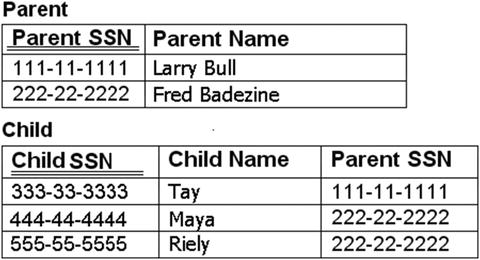
Figure 1-2. Sample Parent and Child tables
In the Child table, the Parent SSN is the foreign key (denoted in these little diagrams using a double line). It is used in a Child row to associate the child with the parent. From these tables, you can see that Tay’s dad is Larry Bull, and the parent of Maya is Fred Badezine (oh, the puns!).
Cardinality is the next question. It is important when defining a relationship to know how many parent rows can relate to how many child rows. Based on the fact that the Parent entity has its key migrated to the Child entity, we have the following restriction: one parent can have any number of children, even zero, based on whether the relationship is considered optional (which we will get to later in the chapter). Of course, if this were really a parent–child human relationship, we could not limit parents to one, because every human (still) has two biological parents, and the number of persons considering themselves parents is even more varied. What makes the job of database design challenging and interesting is all of the realities of the world that don’t always fit into nice neat molds.
Relationships can be divided at this point into two basic types based on the number of entities involved in the relationship:
- Binary relationships: Those between two entities
- Nonbinary relationships: Those between more than two entities
The biggest difference between the two types of relationships is that the binary relationship is very straightforward to implement using foreign keys, as we have discussed previously. When more than two entities are involved, we will generally use methods of modeling and implementation to break down the design into a series of binary relationships, without losing fidelity or readability of the original relationship that your customer will expect.
When you are doing your early design, you need to keep this distinction in mind and learn to recognize each of the possible relationships. When I introduce data modeling in Chapter 3, you’ll learn how to represent relationships of many types in a structured representation.
Working with Binary Relationships
The number of rows that may participate in each side of the relationship is known as the cardinality of the relationship. Different cardinalities of binary relationships will be introduced in this section:
- One-to-many relationship: A relationship linking one instance of an entity with (possibly) multiple instances of another entity. This is the type of relationship that we will implement in our database’s tables.
- Many-to-many relationship: Generally, a relationship where one instance in one entity can be linked with multiple instances of the second entity, and instances in the second entity can in turn be related to many instances in the first one. This is the most typical relationship type to occur in reality.
While all relationships you physically implement in your code will be one-to-many, the real world is not so clear. Consider a football player’s relationship to teams. One team has many players, and a player can play on one team. But a player over their career can play for many teams. So the player-to-team relationship is also a many-to-many relationship. Parent to child, as we previously discussed, is a many-to-many relationship because two biological parents may have many children.
We will look at each of these relationship types and their different subtypes has specific uses and specific associated challenges.
One-to-many relationships are the class of relationships whereby one entity migrates its primary key to another as a foreign key. As discussed earlier, this is commonly referred to as a parent/child relationship and concerns itself only with the relationship between exactly two entities. A child may have, at most, one parent, but a parent may have one or more than one child instances. The generic name of parent/child relationships is one-to-many, but when implementing the relationship, a more specific specification of cardinality is very common, where the one part of the name really can mean zero or one (but never greater than one, as that will be a different type called a many-to-many relationship), and “many” can mean zero, one, a specific number, or an unlimited number.
It should be immediately clear that when the type of relationship starts with “one-to-,” such as “one-to-many,” one row is related to some number of other rows. However, sometimes a child row can be related to zero parent rows. This case is often referred to as an optional relationship. If you consider the earlier Parent/Child example, if this relationship were optional, a child may exist without a parent. If the relationship between parent and child were optional, it would be OK to have a child named Sonny who did not have a parent (well, as far as the database knows), as shown in Figure 1-3.

Figure 1-3. Sample table including a parentless child
The missing value would typically be denoted by NULL, so the row for Sonny would be stored as (ChildSSN:’666-66-6666’, ChildName:’Sonny’, ParentSSN:NULL). For the general case, we (and most others in normal conversation) will speak in terms of one-to-many relationships, just for ease of discussion. However, in more technical terms, there are several different variations of the zero or one-to-(blank) theme that have different implications later, during implementation, that we will cover in this section:
- One-to-many: This is the general case, where “many” can be between zero and infinity.
- One–to–exactly N: In this case, one parent row is required to be related to a given number of child rows. For example, a child must have two biological parents, so it would be one-to-exactly 2 (though discussion about whether both parents must be known to record a child’s existence is more of a topic for Chapter 2, when we discuss requirements. The common exact case is one-to-one).
- One–to–between X and Y: Usually, the case that X is 0 and Y is some boundary set up to make life easier. For example, a user may have between 1 and 2 usernames.
One-to-Many (The General Case)
The one-to-many relationship is the most common and most important relationship type. For each parent row, there may exist unlimited child rows. An example one-to-many relationship might be Customer to Orders, as illustrated in Figure 1-4.

Figure 1-4. One-to-many example
A special type of one-to-many relationship is a “recursive relationship.” In a recursive relationship, the parent and the child are from the same entity, and often the relationship is set up as a single entity. This kind of relationship is used to model a tree data structure. As an example, consider the classic example of a bill of materials. Take something as simple as a ceiling fan. In and of itself, a ceiling fan can be considered a part for sale by a manufacturer, and each of its components is, in turn, also a part that has a different part number. Some of these components also consist of parts. In this example, the ceiling fan could be regarded as made up of each of its parts, and in turn, each of those parts consists of other parts, and so on. (Note that a bill of materials is a slice of a larger “graph” structure to document inventory, as each part can have multiple uses, and multiple parts. This structure type will be covered in more detail in Chapter 8.)
The following table is a small subset of the parts that make up a ceiling fan. Parts 2, 3, and 4 are all parts of a ceiling fan. You have a set of blades and a light assembly (among other things). Part 4, the globe that protects the light, is part of the light assembly.
Part Number    Description           Used in Part Number
-------------  --------------------  --------------------
1              Ceiling Fan           NULL
2              White Fan Blade Kit   1
3              Light Assembly        1
4              Light Globe           3
5              White Fan Blade       2
To read this data, you would start at Part Number 1, and you can see what parts make up that part, which is a fan blade kit and a light assembly. Now, you have the parts with number 2 and 3, and you can look for parts that make them up, which gets you part number 4 and 5. (Note that the algorithm we just used is known as a breadth-first search, where you get all of the items on a level in each pass though the data. It’s not terribly important at this point, but it will come up in Chapter 8 when we are discussing design patterns.)
Often, some limit to the number of children is required by the situation being modeled or a business rule. So rather than one-to-many (where many is infinity), you may say we only support a specific number of related items. A person playing poker is dealt five cards. Throughout the game the player has between zero and five cards, but never more.
As another example, a business rule might state that a user must have exactly two e-mail addresses so they can be more likely to answer one of the e-mails. Figure 1-5 shows an example of that one-to-exactly two relationship cardinality. It’s not particularly a likely occurrence to have data like this, but you never know whether you need a tool until a customer comes in with some wacky request that you need to fill.

Figure 1-5. Example of a one-to-two relationship
The most typical version of a one–to–N relationship type that gets used is a one-to-one relationship. This indicates that for any given parent, there may exist exactly one instance of the child. A one-to-one relationship may be a simple attribute relationship (e.g., a house has a location), or it may be what is referred to as an “is a” relationship. “Is a” relationships indicate that one entity is an extension of another. For example, say there exists a person entity and an employee entity. Employees are all people (in most companies), thus they need the same attributes as people, so we will use a one-to-one relationship: employee is a person. It would be illogical (if not illegal with the labor authorities) to say that an employee is more than one person or that one person is two employees. These types of “is a” relationships are often what are called subtype relationships, something we will cover again later in the book.
Many-to-Many Relationships
The final type of binary relationship is the many-to-many relationship. Instead of a single parent and one or more children, you have two entities where each instance in both entities can be tied to any number of instances in the other. For example, continuing with the familial relationships, a child always has two biological parents—perhaps unknown, but they do exist. This mother and father may have more than one child, and each mother and father can have children from other relationships as well.
Many-to-many relationships make up a lot more of what we will model than you might immediately expect. Consider a car dealer. The car dealer sells cars. Inversely, pick nearly any single model of car, and you’ll see that it is sold by many different car dealers. Similarly, the car dealer sells many different car models. So many car models are sold by many car dealers, and vice versa.
As another example, it seems that relationships like an album’s relationship to a song is simply one-to-many when you begin defining your entities, yet a song can be on many albums. Once you start to include concepts such as singers, musicians, writers, and so on, into the equation, you will see that it requires a lot of many-to-many relationships to adequately model those relationships (many singers to a song, many songs to a singer, etc.). An important part of the design phase is going to be to examine the cardinality of your relationships and make sure you have considered how entities relate to one another in reality, as well as in your computer system.
The many-to-many relationship is not directly implementable using a simple SQL relationship but is typically implemented by introducing another structure to implement the relationship. Instead of the key from one entity being migrated to the other, the keys from both objects in the relationship are migrated to a new entity that is used to implement the relationship (and likely record information about the nature of the relationship as well). In Chapter 3, I’ll present more examples and discuss how to implement the many-to-many relationship.
Working with Nonbinary Relationships
Nonbinary relationships involve more than two entities in the relationship. Nonbinary relationships can be very problematic to discover and model properly, yet they are far more common than you might expect, for example:
A room is used for an activity in a given time period.
Publishers sell books through bookstores and online retailers.
Consider the first of these. We start by defining entities for each of the primary concepts mentioned—room, activity, and time period:
Room (room_number)
Activity (activity_name)
Time_Period (time_period_name)
Next, each of these will be connected in one entity to associate them all into one relationship:
Room_Activity_TimePeriod (room number, activity_name, time_period_name)
We now have an entity that seemingly represents the relationship of room, activity, and time utilization. From there, it may or may not be possible to break down the relationships between these three entities (commonly known as a ternary relationship, because of the three entities) further into a series of relationships between the entities that will satisfy the requirements in an easy-to-use manner. Often, what starts out as a complex ternary relationship is actually discovered to be a series of binary relationships that are easy to work with. This is part of the normalization process that will be covered in Chapter 5 that will change our initial entities into something that can be implemented as tables in SQL. During the early, conceptual phases of design, it is enough to simply locate the existence of the different types of relationships.
Understanding Functional Dependencies
Beyond basic database concepts, I want to introduce a few mathematical concepts now before they become necessary later. They center on the concept of functional dependencies. The structure of a database is based on the idea that given one value (as defined earlier, a key value), you can find related values. For a real-world example, take a person. If you can identify the person, you can also determine other information about the person (such as hair color, eye color, height, or weight). The values for each of these attributes may change over time, but when you ask the question, there will be one and only one answer to the question. For example, at any given instant, there can be only one answer to the question, “What is the person’s eye color?”
We’ll discuss two different concepts related to this in the sections that follow: functional dependencies and determinants. Each of these is based on the idea that one value depends on the value of another.
Understanding Functional Dependencies
Functional dependency is a very simple but important concept. It basically means that if you can determine the value of variable A given a value of variable B, B is functionally dependent on A. For example, say you have a function, and you execute it on one value (let’s call it Value1), and the output of this function is always the same value (Value2). Then Value2 is functionally dependent on Value1. Then if you are certain that for every input to the function (Value1-1, Value1-2, …, Value 1-N) that you will always get back (Value2-1, Value2-2, …, Value 2-N), the function that changes Value1 to Value2 is considered “deterministic.” On the other hand, if the value from the function can vary for each execution, it is “nondeterministic.” This concept is central to how we form a database to meet a customer’s needs, along with the needs of an RDBMS engine.
In a table form, consider the functional dependency of nonkey columns to key columns. For example, consider the following table T with a key of column X:
X     Y
---   ---
1     1
2     2
3     2
You can think of column Y as functionally dependent on the value in X, or fn(X) = Y. Clearly, Y may be the same for different values of X, but not the other way around (note that these functions are not strictly math; it could be IF X = (2 or 3) THEN 2 ELSE 1 that forms the function in question). This is a pretty simple yet important concept that needs to be understood.
X     Y    Z
---   ---  ---
1     1    20
2     2    4
3     2    4
Determining what is a dependency and what is a coincidence is something to be careful of as well. In this example, fn(X) = Y and fn(X) = Y for certain (since that is the definition of a key), but looking at the data, there also appears to exist another dependency in this small subset of data, fn(Y) = Z. Consider that fn(Y) = Z, and you want to modify the Z value to 5 for the second row:
X     Y    Z
---   ---  ---
1     1    20
2     2    5
3     2    4
Now there is a problem with our stated dependency of fn(Y) = Z because fn(2) = 5 AND fn(2) = 4. As you will see quite clearly in Chapter 5, poorly understood functional dependencies are at the heart of many database problems, because one of the primary goals of any database design is that to make one change to a piece of data you should not need to modify data in more than one place. It is a fairly lofty goal, but ideally, it is achievable with just a little bit of planning.
Finding Determinants
A term that is related to functional dependency is “determinant,” which can be defined as “any attribute or set of attributes on which any other attribute or set of attributes is functionally dependent.” In our previous example, X would be considered the determinant. Two examples of this come to mind:
- Consider a mathematical function like 2 * X. For every value of X, a particular value will be produced. For 2, you will get 4; for 4, you will get 8. Anytime you put the value of 2 in the function, you will always return a 4, so 2 functionally determines 4 for function (2 * X). In this case, 2 is the determinant.
- In a more database-oriented example, consider the serial number of a product. From the serial number, additional information can be derived, such as the model number and other specific, fixed characteristics of the product. In this case, the serial number functionally determines the specific, fixed characteristics, and as such, the serial number is the determinant.
If this all seems familiar, it is because any key of a entity will functionally determine the other attributes of the entity, and each key will be a determinant, since it functionally determines the attributes of the entity. If you have two keys, such as the primary key and alternate key of the entity, each must be a determinant of the other.
Relational Programming
One of the more important aspects of relational theory is that there must be a high-level language through which data access takes place. As discussed earlier in this chapter, Codd’s fifth rule states that “…there must be at least one language whose statements are expressible, per some well-defined syntax, as character strings and whose ability to support all of the following is comprehensive: data definition, view definition, data manipulation (interactive and by program), integrity constraints, authorization, and transaction boundaries (begin, commit, and rollback).”
This language has been standardized over the years as the SQL we know (and love!). Throughout this book, we will use most of the capabilities of SQL in some way, shape, or form, because any discussion of database design and implementation is going to be centered on using SQL to do all of the things listed in the fifth rule and more.
There are two characteristics of SQL that are particularly important to understand. First, SQL is at its core a declarative language, which basically means that the goal is to describe what you want done to the computer, and SQL works out the details.1 So when you make the request “Give me all of the data about people,” you ask SQL in a structured version of that very sentence, rather than describe each individual step in the process.
Second, SQL is a relational language, in that you work at the relation (or table) level on sets of data at a time, rather than on one piece of data at a time. This is an important concept. Recall that Codd’s seventh rule states “[t]he capability of handling a base relation or a derived relation as a single operand applies not only to the retrieval of data but also to the insertion, update, and deletion of data.”
What is amazingly cool about SQL as a language is that one very simple declarative statement almost always represents hundreds and thousands of lines of code being executed. Much of this code executes in the hardware realm, accessing data on disk drives, moving that data into registers, and performing operations in the CPU.
If you are already well versed as a programmer in a procedural language like C#, FORTRAN, VB.NET, etc., SQL is a lot more restrictive in what you can do. You have two sorts of high-level commands:
- Data Definition Language (DDL): SQL statements used to set up data storage (tables and the underlying storage), apply security, and so on.
- Data Manipulation Language (DML): SQL statements used to create, retrieve, update, and delete data that has been placed in the tables. In this book, I assume you have used SQL before, so you know that most everything done is handled by four statements: SELECT, INSERT, UPDATE, and DELETE.
As a relational programmer, your job is to give up control of all of the details of storing data, querying data, modifying existing data, and so on. The system (commonly referred to as the relational engine) does the work for you—well, a lot of the work for you. Even more important is as a relational data designer, it is your job to make sure the database suits the needs of the RDBMS. Think of it like a chef in a kitchen. Producing wonderful food is what they do best, but if you arranged their utensils in a random order, it would take a lot longer to make dinner for you.
Dr. David DeWitt (a technical fellow in the Data and Storage Platform Division at Microsoft Corporation) said, during his PASS Keynote in 2010, that getting the RDBMS to optimize the queries you send isn’t rocket science; it is far more difficult than that, mostly because people throw ugly queries at the engine and expect perfection. Consider it like the controls on your car. To go to the grocery store and get milk, you don’t need to know about the internal combustion engine or how electric engines work. You turn the car on, put it in gear, press pedal, and go.
The last point to make again ties back to Codd’s rules, this time the twelfth, the nonsubversion rule. Basically, it states that the goal is to do everything in a language that can work with multiple rows at a time and that low-level languages shouldn’t be able to bypass the integrity rules or constraints of the engine. In other words, leave the control to the engine and use SQL. Of course, this rule does not preclude other languages from existing. The twelfth rule does state that all languages that act on the data must follow the rules that are defined on the data. In some relational engines, it can be faster to work with rows individually rather than as sets. However, the creators of the SQL Server engine have chosen to optimize for set-based operations. This leaves the onus on the nonrelational programmer to play nice with the relational engine and let it do a lot of the work.
Outlining the Database-Specific Project Phases
As we go though the phases of a project, the phases of a database project have some very specific names that have evolved to describe the models that are created. Much like the phases of the entire project, the phases that you will go through when designing a database are defined specifically to help you think about only what is necessary to accomplish the task at hand.
Good design and implementation practices are essential for getting to the right final result. Early in the process, your goals should simply be to figure out the basics of what the requirements are asking of you. Next, think about how to implement using proper fundamental techniques, and finally, tune the implementation to work in the real world.
The process I outline here steers us through creating a database by keeping the process focused on getting things done right, using terminology that is reasonably common in the general practicing programmer community:
- Conceptual: During this phase, the goal is a sketch of the database that you will get from initial requirements gathering and customer information. I said Phase, you identify what the user wants at a high level. You then capture this information in a data model consisting of high-level entities and the relationships between them. (The name “conceptual” is based in finding concepts, not a design that is conceptual. Think of them like storyboards of a movie. They storyboard to make sure everything seems to work together, and if not, changes require an eraser, not completely reshooting a film. )
- Logical: The logical phase is an implementation-nonspecific refinement of the work done in the conceptual phase, transforming the concepts into a full-fledged relational database design that will be the foundation for the implementation design. During this stage, you flesh out the model that the system needs and capture all of the data business rules that will need to be implemented. (Following the movie analogy, this is where the “final” script is written, actors are hired, etc.)
- Physical: In this phase, you adapt the logical model for implementation to the host RDBMS, in our case, SQL Server. For the most part, the focus in this phase is to build a solution to the design that matches the logical phase output. However, a big change has occurred in recent years, and that is based on SQL Server internals. We will need to choose between a few models of implementation during the physical phase. (The physical database is like the movie now in the can, ready to be shown in theaters. The script may change a bit, but overall it will be very close.)
- Engine adjustment: In this phase, you work with the model where the implementation data structures are mapped to storage devices. This phase is also more or less the performance tuning/optimization/adaption phase of the project, because it is important that your implementation should function (in all ways except performance) the same way no matter what the hardware/client software looks like. It might not function very fast, but it will function. During this phase of the project indexes, disk layouts, are adjusted to make the system run faster, without changing the meaning of the system. (The engine adjustment phase of the project is like distributing a film out to millions of people to watch on different screens, different sized theaters, formats, etc. It is the same film on a massive screen as on your phone screen, with optimizations made so it works in each situation.)
You may be questioning at this point, “What about testing? Shouldn’t there be a testing phase?” Yes, each of the phases includes testing. You test the conceptual design to make sure it fits the requirements. You test the logical design to make sure you have covered every data point that the user required. You test the physical design by building code and unit and scenario testing it. You test how your code works in the engine by throwing more data at the database than you will ever see in production and determining whether the engine can handle it as is or requires adjustments. A specific testing phase is still necessary for the overall application, but each of the database design/implementation phases should have testing internally to the process (something that will equally be sewn into the rest of the book as we cover the entire process).
Conceptual Phase
The conceptual design phase is essentially a process of analysis and discovery; the goal is to define the organizational and user data requirements of the system. Note that parts of the overall design picture beyond the needs of the database design will be part of the conceptual design phase (and all follow-on phases), but for this book, the design process will be discussed in a manner that may make it sound as if the database is all that matters (as a reader of this book who is actually reading this chapter on fundamentals, you probably feel that way already).
Over the years, I have discovered that the term “conceptual model” has several meanings depending on the person I interviewed about the subject. In some people’s eyes, the conceptual model was no more than a diagram of entities and relationships. Others included attributes and keys as they were describing it.
The core activity that defines the conceptual modeling process for every source I have found is discovering and documenting a set of entities and the relationships between if possible them, the goal being to capture, at a high level, the fundamental concepts that are required to support the business processes and users’ needs. Entity discovery is at the heart of this process. Entities correspond to nouns (people, places, and things) that are fundamental to the business processes you are trying to improve by creating software.
Beyond this, how much more you model or document is very much debatable. The people I have worked with have almost always documented as much of the information as they can in the model as they find it. I personally find the discipline of limiting the model to entities and relationships to be an important first step, and invariably the closer I get to a correct conceptual model, the shorter the rest of the process is.
Logical Phase
The logical phase is a refinement of the work done in the conceptual phase. The output from this phase will be an essentially complete blueprint for the design of the relational database. Note that during this stage, you should still think in terms of entities and their attributes, rather than tables and columns, though in the database’s final state there may be basically no difference. No consideration should be given at this stage to the exact details of how the system will be implemented. As previously stated, a good logical design could be built on any RDBMS. Core activities during this stage include the following:
- Drilling down into the conceptual model to identify the full set of entities that will be required to define the entire data needs of the user.
- Defining the attribute set for each entity. For example, an Order entity may have attributes such as Order Date, Order Amount, Customer Name, and so on.
- Identifying the attributes (or a group of attributes) that make up candidate keys. This includes primary keys, foreign keys, surrogate keys, and so on.
- Defining relationships and associated cardinalities.
- Identifying an appropriate domain (which will become a datatype) for each attribute including whether values are required.
While the conceptual model was meant to give the involved parties a communication tool to discuss the data requirements and to start seeing a pattern to the eventual solution, the logical phase is about applying proper design techniques. The logical modeling phase defines a blueprint for the database system, which can be handed off to someone else with little knowledge of the system to implement using a given technology (which in our case is going to be some version of Microsoft SQL Server).
![]() Note Before we begin to build the logical model, we need to introduce a complete data modeling language. In our case, we will be using the IDEF1X modeling methodology, described in Chapter 3.
Note Before we begin to build the logical model, we need to introduce a complete data modeling language. In our case, we will be using the IDEF1X modeling methodology, described in Chapter 3.
Physical
During the physical implementation phase, you fit the logical design to the tool that is being used (in our case, the SQL Server RDBMS). This involves validating the design (using the rules of what is known as normalization, covered in Chapter 5), then choosing datatypes for columns to match the domains, building tables, applying constraints and occasionally writing triggers to implement business rules, and so on to implement the logical model in the most efficient manner. This is where reasonably deep platform-specific knowledge of SQL Server, T-SQL, and other technologies becomes essential.
Occasionally, this phase can entail some reorganization of the designed objects to make them easier to implement in the RDBMS. In general, I can state that for most designs there is seldom any reason to stray a great distance from the logical model, though the need to balance user load, concurrency needs, and hardware considerations can make for some changes to initial design decisions. Ultimately, one of the primary goals is that no data that has been specified or integrity constraints that have been identified in the conceptual and logical phases will be lost. Data points can (and will) be added, often to handle the process of writing programs to use the data, like data to know who created or was the last person to change a row. The key is to avoid affecting the designed meaning or, at least, not to take anything away from that original set of requirements.
At this point in the project, constructs will be applied to handle the business rules that were identified during the conceptual part of the design. These constructs will vary from the favored declarative constraints, such as defaults and check constraints, to less favorable but still useful triggers and occasionally stored procedures. Finally, this phase includes designing the security for the data we will be storing (though to be clear, we may design security last, we shouldn’t design it after you finish coding, in case it affects the design in some way).
Engine Adjustment Phase
The goal of the storage layout phase is to optimize how your design interacts with the relational engine—for example, by implementing effective data distribution on the physical disk storage and by judicious use of indexes, or perhaps changing to use the columnstore or in-memory structures that Microsoft has implemented in the past few years (and has significantly improved in SQL Server 2016 with columnstore indexes that can be used for reporting on OLTP tables without blocking writers, editable columnstore indexes, and other new features). While the purpose of the RDBMS is to largely isolate us from the physical aspects of data retrieval and storage, in this day and age it is still very important to understand how SQL Server physically implements the data storage to optimize database access code.
During this stage, the goal is to optimize performance without changing the implemented database in any way to achieve that aim. This goal embodies Codd’s eleventh rule, which states that an RDBMS should have distribution independence. Distribution independence implies that users should not have to be aware of whether a database is distributed. Distributing data across different files, or even different servers, may be necessary, but as long as the published physical object names do not change, users will still access the data as columns in rows in tables in a database.
As more and more data is piled into your database, ideally the only change you will need to make to your database is in this phase (assuming the requirements never change, which is reasonably unlikely for most people). This task is very often one for the production DBA, who is charged with maintaining the database environment. This is particularly true when the database system has been built by a third party, like in a packaged project or by a consultant.
![]() Note Our discussion of the storage model will be reasonably limited. We will start by looking at entities and attributes during conceptual and logical modeling. In implementation modeling, we will switch gears to deal with tables, rows, and columns. The physical modeling of records and fields will be dealt with only briefly (in Chapter 8). If you want a deeper understanding of the physical implementation, check out the latest in the Internals series by Kalen Delaney (http://sqlserverinternals.com/). To see where the industry is rapidly headed, take a look at the SQL Azure implementation, where the storage aspects of the implementation are very much removed from your control and even grasp.
Note Our discussion of the storage model will be reasonably limited. We will start by looking at entities and attributes during conceptual and logical modeling. In implementation modeling, we will switch gears to deal with tables, rows, and columns. The physical modeling of records and fields will be dealt with only briefly (in Chapter 8). If you want a deeper understanding of the physical implementation, check out the latest in the Internals series by Kalen Delaney (http://sqlserverinternals.com/). To see where the industry is rapidly headed, take a look at the SQL Azure implementation, where the storage aspects of the implementation are very much removed from your control and even grasp.
Summary
In this chapter, I offered a quick history to provide context to the trip I will take you on in this book, along with some information on the basic concepts of database objects and some aspects of theory. It’s very important that you understand most of the concepts discussed in this chapter, since from now on, I’ll assume you understand them, though to be honest, all of the really deeply important points seem to come up over and over and over throughout this book. I pretty much guarantee that the need for a natural key on every table (in the resulting database that is obviously your goal for reading this far in the book) will be repeated enough that you may find yourself taking vacations to the Florida Keys and not even realize why (hint, it could be the natural Key beauty that does it to you).
I introduced relational data structures and defined what a database is. Then, we covered tables, rows, and columns. From there, I explained the information principle (which states that data is accessible only in tables and that tables have no order), defined keys, and introduced NULLs and relationships. We also looked at a basic introduction to the impetus for how SQL works.
We discussed the concept of dependencies, which basically are concerned with noticing when the existence of a certain value requires the existence of another value. This information will be used again in Chapter 5 as we reorganize our data design for optimal usage in our relational engine.
In the next few chapters, as we start to formulate a conceptual and then a logical design, we will primarily refer to entities and their attributes. After we have logically designed what our data ought to look like, we’ll shift gears to the implementation phase and speak of tables, rows, and columns. The terminology is not terribly important, and in the real world it is best not to be a terminology zealot, but when learning, it is a good practice to keep the differences distinct. The really exciting part comes as database construction starts, and our database starts to become real. After that, all that is left is to load our data into a well-formed, well-protected relational database system and set our users loose!
Everything starts with the fundamentals presented here, including understanding what a table is and what a row is (and why it differs from a record). As a last not-so-subtle-subliminal reminder, rows in tables have no order, and tables need natural keys.
The rest of the book will cover the process with the following phases in mind (the next chapter will be a short coverage of the project phase that comes just before you start the conceptual design requirements):
- Conceptual: Identify the concepts that the users expect to get out of the database system that you are starting to build.
- Logical: Document everything that the user will need in their database, including data, predicates/rules, etc.
- Physical: Design and implement the database in terms of the tools used (in the case of this book, SQL Server), making adjustments based on the realities of the current version of SQL Server/other RDBMS you are working with.
- Engine adjustment: Design and lay out the data on storage based on usage patterns and what works best for SQL Server. Adjust the design such that it works well with the engine layers, both algorithms and storage layers. The changes made ought to only affect performance, not correctness.
Of course, the same person will not necessarily do every one of these steps. Some of these steps require different skill sets, and not everyone can know everything—or so I have been told.
________________
1For a nice overview of declarative languages, see https://www.britannica.com/technology/declarative-language.