
A general neural net is shown in Figure 7.1. This is a “deep learning” neural net because it has multiple internal layers.

Figure 7.1 Deep learning neural net.
A convolutional neural network is a pipeline with multiple stages. The images go into one end and the probability that the image is a cat comes out the other. There are three types of layers:
Convolutional layers (hence the name)
Pooling layers
Fully connected layers
A convolutional neural net is shown in Figure 7.6. This is also a “deep learning” neural net because it has multiple internal layers, but now the layers are of the three types described above.

Figure 7.2 Deep learning convolutional neural net [1].
We can have as many layers as we want. A neuron in a neural net is ![]() (7.1)
(7.1)
where w is a weight, b is a bias, and σ() is the nonlinear function that operates on the input wx + b. This is the activation function. There are many possible sigmoid functions.
A sigmoid or hyperbolic tangent is often used as the activation function. The function Activation generates activation functions.

Figure 7.3 shows the three activation functions with k=1. A third is the rectified linear output function or

Figure 7.3 Activation function.
 (7.2) This seems a bit strange for an image processing network where the inputs are all positive. However, the bias term can make the argument negative and previous layers may also change the sign.
The following recipes will detail each step in the chain. We will start with gathering image data. We will then describe the convolution process. The next recipe will implement pooling. We will show a recipe for Softmax. We will then demonstrate the full network using random weights. Finally, we will train the network using a subset of the images and see if we can identify the other images.
7.1 Obtain Data Online: For Training a Neural Network
7.1.1 Problem
We want to find photographs online for training a face recognition neural net.
7.1.2 Solution
Go to ImageNet to find images.
7.1.3 How It Works
ImageNet, http://www.image-net.org , is an image database organized according to the WordNet hierarchy. Each meaningful concept in WordNet is called a “synonym set.” There are more than 100,000 sets and 14 million images in ImageNet. For example, type in “Siamese cat.” Click on the link. You will see 445 images. You’ll notice that there are a wide variety of shots from many angles and a wide range of distances.
Synset: Siamese cat, Siamese
Definition: a slender, short-haired, blue-eyed breed of cat having a pale coat with dark ears, paws, face, and tail tip.
Popularity percentile:: 57%
Depth in WordNet: 8
This is a great resource! However, we are going to instead use pictures of our cats for our test to avoid copyright issues.
7.2 Generating Data for Training a Neural Net
7.2.1 Problem
We want grayscale photographs for training a face recognition neural net.
7.2.2 Solution
Take photographs using a digital camera.
7.2.3 How It Works
We first take pictures of several cats. We’ll use them to train the net. The photos are taken using an iPhone 6. We take just facial photos; to make the problem easier, we limit the photos to facial shots of the cats. We then frame the shots so that they are reasonably consistent in size and minimize the background. We then convert them to grayscale.
We use the function ImageArray to read in the images. It takes a path to a folder containing the images to be processed.


The function has a demo with our local folder of cat images.

ImageArray uses averages the three colors to convert the color images to grayscale. It flips them upside down since the image coordinates are opposite that of MATLAB. We used GraphicConverter 10 TM to crop the images around the cat’s face and make them all 1024 x 1024 pixels. One of the challenges of image matching is to do this process automatically. Also, training typically uses thousands of images. We are using just a few to see if our neural net can determine if the test image is a cat, or even one we have used in training! ImageArray scales the image using the function ScaleImage


Notice that it creates the new image array as uint8. Figure 7.4 shows the results of scaling.

Figure 7.4 Image scaled from 1024 × 1024 to 256 × 256.
The images are shown in Figure 7.5.

Figure 7.5 (64 × 64)-pixel grayscale cat images.
7.3 Convolution
7.3.1 Problem
We want to implement convolution to reduce the number of weights in the network.
7.3.2 Solution
Implement convolution using MATLAB matrix operations.
7.3.3 How It Works
We create an n-x-n mask that we apply to the input matrix. The matrix dimensions are m x m, where m is greater than n. We start in the upper left corner of the matrix. We multiply the mask times the corresponding elements in the input matrix and do a double sum. That is the first element of the convolved output. We then move it column by column until the highest column of the mask is aligned with the highest column of the input matrix. We then return it to the first column and increment the row. We continue until we have traversed the entire input matrix and our mask is aligned with the maximum row and maximum column.
The mask represents a feature. In effect, we are seeing if the feature appears in different areas of the image. We can have multiple masks. There are one bias and one weight for each element of the mask for each feature. In this case, instead of 16 sets of weights and biases, we only have 4. For large images, the savings can be substantial. In this case the convolution works on the image itself. Convolutions can also be applied to the output of other convolutional layers or pooling layers, as shown in Figure 7.6.

Figure 7.6 Convolution process showing the mask at the beginning and end of the process.
Convolution is implemented in Convolve.m.
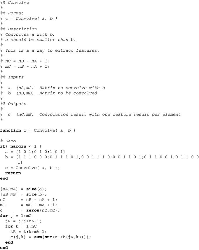
The demo produces the following results.
>> Convolve
a =
1 0 1
0 1 0
1 0 1
b =
1 1 1 0 0 0
0 1 1 1 0 1
0 0 1 1 1 0
0 0 1 1 0 1
0 1 1 0 0 1
0 1 1 0 0 1
ans =
4 3 4 1
2 4 3 5
2 3 4 2
3 3 2 3
7.4 Convolution Layer
7.4.1 Problem
We want to implement a convolution connected layer.
7.4.2 Solution
Use code from Convolve to implement the layer.
7.4.3 How It Works
The “convolution” neural net scans the input with the mask. Each input to the mask passes through an activation function that is identical for a given mask. This reduces the number of weights.


Figure 7.7 shows the inputs and outputs from the demo. The tanh activation function is used in this demo. The weights and biases are random.

Figure 7.7 Inputs and outputs for the convolution layer.
7.5 Pooling
7.5.1 Problem
We want to pool the outputs of the convolution layer to reduce the number of points we need to process.
7.5.2 Solution
Implement a function to take the output of the convolution function.
7.5.3 How It Works
Pooling layers take a subset of the outputs of the convolutional layers and pass that on. They do not have any weights. Pooling layers can use the maximum value of the pool or take the median or mean value. Our pooling function has all there as an option. The pooling function divides the input into n x n subregions and returns an n x n matrix.
Pooling is implemented in Pool.m. Notice we use str2func instead of a switch statement.

The demo produces the following results.
The built-in demo creates 4 pools from an 4 x 4 matrix.
>> Pool
a =
0.9031 0.7175 0.5305 0.5312
0.1051 0.1334 0.8597 0.9559
0.7451 0.4458 0.6777 0.0667
0.7294 0.5088 0.8058 0.5415
ans =
0.4648 0.7193
0.6073 0.5229
7.6 Fully Connected Layer
7.6.1 Problem
We want to implement a fully connected layer.
7.6.2 Solution
Use Activation to implement the network.
7.6.3 How It Works
The “fully connected” neural net layer is the traditional neural net where every input is connected to every output as shown in Figure 7.8.

Figure 7.8 Fully connected neural net. This shows only one output.
We implement the fully connected network with n inputs and m outputs. Each path to an output can have a different weight and bias. FullyConnectedNN can handle any number of inputs or outputs.


Figure 7.9 shows the outputs from the demo. The tanh activation function is used in this demo. The weights and biases are random. The change in shape from input to output is the result of the activation function.

Figure 7.9 The two outputs from the demo function are shown vs. the two inputs.
7.7 Determining the Probability
7.7.1 Problem
We want to get a probability from neural net outputs.
7.7.2 Solution
Implement the Softmax function. This will be used for the output nodes of our network.
7.7.3 How It Works
Given a set of inputs, the Softmax function, a generalization of the logistic function, calculates a set of positive values p that add to 1. It is  (7.3)
(7.3)
where q are the inputs and N is the number of inputs.
The function is implemented in Softmax.m.
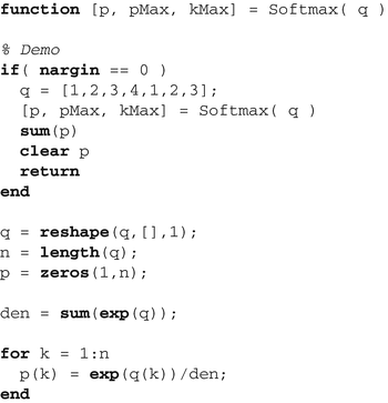
The results of the demo are
>> Softmax
p =
0.0236 0.0643 0.1747 0.4748 0.0236 0.0643 0.1747
pMax =
0.4748
kMax =
4
ans =
1.0000
The last number is the sum of p, which should be (and is) 1.
7.8 Test the Neural Network
7.8.1 Problem
We want to integrate convolution, pooling, a fully connected layer, and Softmax.
7.8.2 Solution
The solution is write a convolutional neural net. We integrate the convolution, pooling, fully connected net, and Softmax functions. We then test it with randomly generated weights.
7.8.3 How It Works
Figure 7.10 shows the image processing neural network. It has one convolutional layer, one pooling layer, and a fully connected layer, and the final layer is the Softmax.
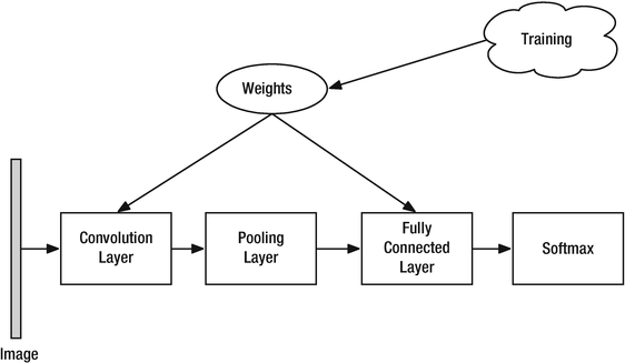
Figure 7.10 Neural net for the image processing.
>> TestNN
Image IMG_3886.png has a 13.1% chance of being a cat
As expected, the neural net does not identify the cat! The code in ConvolutionNN that performs the test is shown below.

Figure 7.11 shows the output of the various stages.

Figure 7.11 Stages in the convolutional neural net processing.
7.9 Recognizing an Image
7.9.1 Problem
We want to determine if an image is that of a cat.
7.9.2 Solution
We train the neural network with a series of cat images. We then use one picture from the training set and a separate picture and compute the probabilities that they are cats.
7.9.3 How It Works
We run the script TrainNN to see if the input image is a cat.

The script returns that the image is probably a cat.
>> TrainNN
Image IMG_3886.png has a 56.0% chance of being a cat
We can improve the results with
More images
More features (masks)
Changing the connections in the fully connected layer
Adding the ability of ConvolutionalNN to handle RGB images directly
Changing ConvolutionalNN
Summary
This chapter has demonstrated facial recognition using MATLAB. Convolutional neural nets were used to process pictures of cats for learning. When trained, the neural net was asked to identify other pictures to determine if they were pictures of a cat. Table 7.1 lists the code introduced in this chapter.
Table 7.1 Chapter Code Listing
File | Description |
|---|---|
Activation | Generate activation functions |
ImageArray | Read in images in a folder and convert to grayscale |
ConvolutionalNN | Implement a convolutional neural net |
ConvolutionLayer | Implement a convolutional layer |
Convolve | Convolve a two-dimensional array using a mask |
Pool | Pool a two-dimensional array |
FullyConnectedNN | Implement a fully connected neural network |
ScaleImage | Scale an image |
Softmax | Implement the Softmax function |
TrainNN | Train the convolutional neural net |
TestNN | Test the convolutional neural net |
TrainingData.mat | Data from TestNN |
[1] Matthijs Hollemans. Convolutional neural networks on the iPhone with VGGNet. http://matthijshollemans.com/2016/08/30/vggnet-convolutional-neural-network-iphone/ , 2016.