
1.1 Introduction
Machine learning is a field in computer science where existing data are used to predict, or respond to, future data. It is closely related to the fields of pattern recognition, computational statistics, and artificial intelligence. Machine learning is important in areas like facial recognition, spam filtering, and others where it is not feasible, or even possible, to write algorithms to perform a task.
For example, early attempts at spam filtering had the user write rules to determine what was spam. Your success depended on your ability to correctly identify the attributes of the message that would categorize an email as spam, such as a sender address or subject keyword, and the time you were willing to spend to tweak your rules. This was only moderately successful as spam generators had little difficulty anticipating people’s rules. Modern systems use machine learning techniques with much greater success. Most of us are now familiar with the concept of simply marking a given message as “spam” or “not spam,” and we take for granted that the email system can quickly learn which features of these emails identify them as spam and prevent them from appearing in our inbox. This could now be any combination of IP or email addresses and keywords in the subject or body of the email, with a variety of matching criteria. Note how the machine learning in this example is data-driven, autonomous, and continuously updating itself as you receive email and flag it.
In a more general sense, what does machine learning mean? Machine learning can mean using machines (computers and software) to gain meaning from data. It can also mean giving machines the ability to learn from their environment. Machines have been used to assist humans for thousands of years. Consider a simple lever, which can be fashioned using a rock and a length of wood, or the inclined plane. Both of these machines perform useful work and assist people, but neither has the ability to learn. Both are limited by how they are built. Once built, they cannot adapt to changing needs without human interaction. Figure 1.1 shows early machines that do not learn.

Figure 1.1 Simple machines that do not have the capability to learn.
Both of these machines do useful work and amplify the capabilities of people. The knowledge is inherent in their parameters, which are just the dimensions. The function of the inclined plane is determined by its length and height. The function of the lever is determined by the two lengths and the height. The dimensions are chosen by the designer, essentially building in the designer’s knowledge.
Machine learning involves memory that can be changed while the machine operates. In the case of the two simple machines described above, knowledge is implanted in them by their design. In a sense they embody the ideas of the builder; thus, they are a form of fixed memory. Learning versions of these machines would automatically change the dimensions after evaluating how well the machines were working. As the loads moved or changed, the machines would adapt. A modern crane is an example of a machine that adapts to changing loads, albeit at the direction of a human being. The length of the crane can be changed depending on the needs of the operator.
In the context of the software we will be writing in this book, machine learning refers to the process by which an algorithm converts the input data into parameters it can use when interpreting future data. Many of the processes used to mechanize this learning derive from optimization techniques and in turn are related to the classic field of automatic control. In the remainder of this chapter we will introduce the nomenclature and taxonomy of machine learning systems.
1.2 Elements of Machine Learning
This section introduces key nomenclature for the field of machine learning.
1.2.1 Data
All learning methods are data driven. Sets of data are used to train the system. These sets may be collected by humans and used for training. The sets may be very large. Control systems may collect data from sensors as the systems operate and use that to identify parameters—or train the system.
■ Note When collecting data from training, one must be careful to ensure that the time variation of the system is understood. If the structure of a system changes with time, it may be necessary to discard old data before training the system. In automatic control this is sometimes called a “forgetting factor” in an estimator.
1.2.2 Models
Models are often used in learning systems. A model provides a mathematical framework for learning. A model is human derived and based on human observations and experiences. For example, a model of a car, seen from above, might be that it is rectangular shaped with dimensions that fit within a standard parking spot. Models are usually thought of as human derived and providing a framework for machine learning. However, some forms of machine learning develop their own models without a human-derived structure.
1.2.3 Training
A system that maps an input to an output needs training to do this in a useful way. Just as people need to be trained to perform tasks, machine learning systems need to be trained. Training is accomplished by giving the system an input and the corresponding output and modifying the structure (models or data) in the learning machine so that mapping is learned. In some ways this is like curve fitting or regression. If we have enough training pairs, then the system should be able to produce correct outputs when new inputs are introduced. For example, if we give a face recognition system thousands of cat images and tell it that those are cats, we hope that when it is given new cat images, it will also recognize them as cats. Problems can arise when you don’t give it enough training sets or the training data are not sufficiently diverse, that is, do not represent the full range of cats in this example.
1.2.3.1 Supervised Learning
Supervised learning means that specific training sets of data are applied to the system. The learning is supervised in that the “training sets” are human derived. It does not necessarily mean that humans are actively validating the results. The process of classifying the system’s outputs for a given set of inputs is called labeling. That is, you explicitly say which results are correct or which outputs are expected for each set of inputs.
The process of generating training sets can be time consuming. Great care must be taken to ensure that the training sets will provide sufficient training so that when real-world data are collected the system will produce correct results. They must cover the full range of expected inputs and desired outputs. The training is followed by test sets to validate the results. If the results aren’t good, then the test sets are cycled into the training sets and the process repeated.
A human example would be a ballet dancer trained exclusively in classical ballet technique. If she were then asked to dance a modern dance, the results might not be as good as required because the dancer did not have the appropriate training sets; her training sets were not sufficiently diverse.
1.2.3.2 Unsupervised Learning
Unsupervised learning does not utilize training sets. It is often used to discover patterns in data for which there is no “right” answer. For example, if you used unsupervised learning to train a face identification system, the system might cluster the data in sets, some of which might be faces. Clustering algorithms are generally examples of unsupervised learning. The advantage of unsupervised learning is that you can learn things about the data that you might not know in advance. It is a way of finding hidden structures in data.
1.2.3.3 Semisupervised Learning
With the semisupervised approach, some of the data is in the form of labeled training sets and other data are not [1]. In fact, typically only a small amount of the input data is labeled while most is not, as the labeling may be an intensive process requiring a skilled human. The small set of labeled data is leveraged to interpret the unlabeled data.
1.2.3.4 Online Learning
The system is continually updated with new data [1]. This is called “online” because many of the learning systems use data collected online. It could also be called “recursive learning.” It can be beneficial to periodically “batch” process data used up to a given time and then return to the online learning mode. The spam filtering systems from the introduction utilize online learning.
1.3 The Learning Machine
Figure 1.2 shows the concept of a learning machine. The machine absorbs information from the environment and adapts. Note that inputs may be separated into those that produce an immediate response and those that lead to learning. In some cases they are completely separate. For example, in an aircraft a measurement of altitude is not usually used directly for control. Instead, it is used to help select parameters for the actual control laws. The data required for learning and regular operation may be the same, but in some cases separate measurements or data will be needed for learning to take place. Measurements do not necessarily mean data collected by a sensor such as radar or a camera. It could be data collected by polls, stock market prices, data in accounting ledgers, or data gathered by any other means. The machine learning is then the process by which the measurements are transformed into parameters for future operation.

Figure 1.2 A learning machine that senses the environment and stores data in memory.
Note that the machine produces output in the form of actions. A copy of the actions may be passed to the learning system so that it can separate the effects of the machine actions from those of the environment. This is akin to a feedforward control system, which can result in improved performance.
A few examples will clarify the diagram. We will discuss a medical example, a security system, and spacecraft maneuvering.

Figure 1.3 Taxonomy of machine learning. Optimization is part of the taxonomy because the results of optimization can be new discoveries, such as a new type of spacecraft or aircraft trajectory.
A doctor might want to diagnose diseases more quickly. She would collect data on tests on patients and then collate the results. Patient data might include age, height, weight, historical data like blood pressure readings and medications prescribed, and exhibited symptoms. The machine learning algorithm would detect patterns so that when new tests were performed on a patient the machine learning algorithm would be able to suggest diagnoses or additional tests to narrow down the possibilities. As the machine learning algorithm was used, it would hopefully get better with each success or failure. In this case the environment would be the patients themselves. The machine would use the data to generate actions, which would be new diagnoses. This system could be built in two ways. In the supervised learning process, test data and known correct diagnoses would be used to train the machine. In an unsupervised learning process, the data would be used to generate patterns that might not have been known before, and these could lead to diagnosing conditions that would normally not be associated with those symptoms.
A security system might be put into place to identify faces. The measurements are camera images of people. The system would be trained with a wide range of face images taken from multiple angles. The system would then be tested with these known persons and its success rate validated. Those that are in the database should be readily identified and those that are not should be flagged as unknown. If the success rate were not acceptable, more training might be needed or the algorithm itself might need to be tuned. This type of face recognition is now common, used in Mac OS X’s “Faces” feature in Photos and Facebook when “tagging” friends in photos.
For precision maneuvering of a spacecraft, the inertia of the spacecraft needs to be known. If the spacecraft has an inertial measurement unit that can measure angular rates, the inertia matrix can be identified. This is where machine learning is tricky. The torque applied to the spacecraft, whether by thrusters or momentum exchange devices, is only known to a certain degree of accuracy. Thus, the system identification system must sort out, if it can, the torque scaling factor from the inertia. The inertia can only be identified if torques are applied. This leads to the issue of stimulation. A learning system cannot learn if the system to be studied does not have known inputs, and those inputs must be sufficient to stimulate the system so that the learning can be accomplished.
1.4 Taxonomy of Machine Learning
In this book we take a bigger view of machine learning than is normally done. We expand machine learning to include adaptive and learning control. This field started off independently but now is adapting technology and methods from machine learning. Figure 1.3 shows how we organize the technology of machine learning. You will notice that we created a title that encompasses three branches of learning; we call the whole subject area “autonomous learning.” That means learning without human intervention during the learning process.
There are three categories under autonomous learning. The first is control. Feedback control is used to compensate for uncertainty in a system or to make a system behave differently than it would normally behave. If there was no uncertainty, you wouldn’t need feedback. For example, if you are a quarterback throwing a football at a running player, assume for a moment that you know everything about the upcoming play. You know exactly where the player should be at a given time, so you can close your eyes, count, and just throw the ball to that spot. Assuming the player has good hands, you would have a 100% reception rate! More realistically, you watch the player, estimate the player’s speed, and throw the ball. You are applying feedback to the problem. As stated, this is not a learning system. However, if now you practice the same play repeatedly, look at your success rate and modify the mechanics and timing of your throw using that information, you would have an adaptive control system, the second box from the top of the control list. Learning in control takes place in adaptive control systems and also in the general area of system identification. System identification is learning about a system. Optimal control may not involve any learning. For example, what is known as full state feedback produces an optimal control signal but does involve learning. In full state feedback the combination of model and data tells us everything we need to know about the system. However, in more complex systems we can’t measure all the states and don’t know the parameters perfectly, so some form of learning is needed to produce “optimal” results.
The second category of autonomous learning is artificial intelligence. Machine learning traces some of its origins in artificial intelligence. Artificial intelligence is the area of study whose goal is to make machines reason. While many would say the goal is “think like people,” this is not necessarily the case. There may be ways of reasoning that are not similar to human reasoning but are just as valid. In the classic Turing test, Turing proposes that the computer only needs to imitate a human in its output to be a “thinking machine” regardless of how those outputs are generated. In any case, intelligence generally involves learning, and so learning is inherent in many artificial intelligence technologies.
The third category is what many people consider true machine learning. This is making use of data to produce behavior that solves problems. Much of its background comes from statistics and optimization. The learning process may be done once in a batch process or continually in a recursive process. For example, in a stock buying package a developer might have processed stock data for several years, say prior to 2008, and used that to decide which stocks to buy. That software might not have worked well during the financial crash. A recursive program would continuously incorporate new data. Pattern recognition and data mining fall into this category. Pattern recognition is looking for patterns in images. For example, the early AI Blocks World software could identify a block in its field of view. It could find one block in a pile of blocks. Data mining is taking large amounts of data and looking for patterns, for example, taking stock market data and identifying companies that have strong growth potential.
1.5 Autonomous Learning Methods
This section introduces you to popular machine learning techniques. Some will be used in the examples in this book. Others are available in MATLAB products and open-source products.
1.5.1 Regression
Regression is a way of fitting data to a model. A model can be a curve in multiple dimensions. The regression process fits the data to the curve, producing a model that can be used to predict future data. Some methods, such as linear regression or least squares, are parametric in that the number of parameters to be fit are known. An example of linear regression is shown in the listing below and in Figure 1.4. This model was created by starting with the line y = x and adding noise to y. The line was recreated using a least-squares fit via MATLAB’s pinv Pseudoinverse function.
Listing 1.1 Linear Regression
%% LinearRegression Script that demonstrates linear regression
% Fit a linear model to linear or quadratic data
%% Generate the data and perform the regression
% Input
x = linspace(0,1,500)';
n = length(x);
% Model a polynomial, y = ax2 + mx + b
a = 1.0; % quadratic - make nonzero for larger errors
m = 1.0; % slope
b = 1.0; % intercept
sigma = 0.1; % standard deviation of the noise
y0 = a*x.^2 + m*x + b;
y = y0 + sigma*randn(n,1);
% Perform the linear regression using pinv
a = [x ones(n,1)];
c = pinv(a)*y;
yR = c(1)*x + c(2); % the fitted line
%% Generate plots
h = figure('name','Linear␣Regression');
h.Name = 'Linear␣Regression';
plot(x,y); hold on;
plot(x,yR,'linewidth',2);
grid on
xlabel('x');
ylabel('y');
title('Linear␣Regression');
legend('Data','Fit')
figure('Name','Regression␣Error')
plot(x,yR-y0);
grid on
We can solve the problem ![]() (1.1)
(1.1)
by taking the inverse of A if the length of x and b are the same: ![]() (1.2)
(1.2)
This works because A is a square matrix but only works if A is not singular. That is, it has a valid inverse. If the length of x and that of b are the same, we can still find an approximation to x where x = pinv(A)b. For example, in the first case below A is 2 by 2. In the second case, it is 3 by 2, meaning there are 3 elements of x and 2 of b.
>> inv(rand(2,2))
ans =
1.4518 -0.2018
-1.4398 1.2950
>> pinv(rand(2,3))
ans =
1.5520 -1.3459
-0.6390 1.0277
0.2053 0.5899

Figure 1.4 Learning with linear regression.
The system learns the parameters, slope and y-intercept, from the data. The more data, the better the fit. As it happens, our model
![]() (1.3)
(1.3)
is correct. However, if it were wrong, the fit would be poor. This is an issue with model-based learning. The quality of the results is highly dependent on the model. If you are sure of your model, then it should be used. If not, other methods, such as unsupervised learning, may produce better results. For example, if we add the quadratic term x
2 we get the fit in Figure 1.5. Notice how the fit is not as good as we might like.
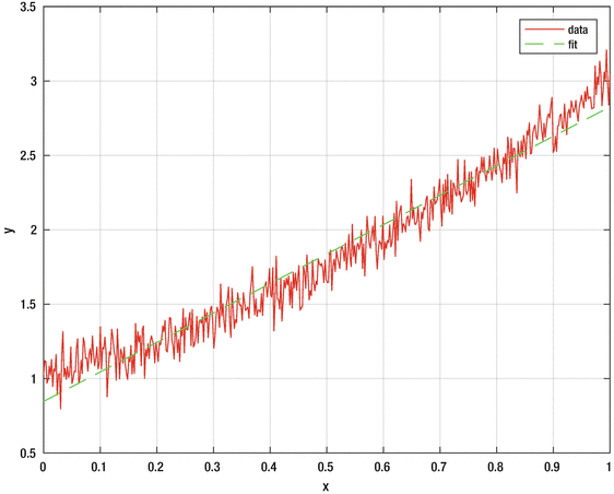
Figure 1.5 Learning with linear regression for a quadratic.
1.5.2 Neural Nets
A neural net is a network designed to emulate the neurons in a human brain. Each “neuron” has a mathematical model for determining its output from its input; for example, if the output is a step function with a value of 0 or 1, the neuron can be said to be “firing” if the input stimulus results in a 1 output. Networks are then formed with multiple layers of interconnected neurons. Neural networks are a form of pattern recognition. The network must be trained using sample data, but no a priori model is required. Networks can be trained to estimate the output of nonlinear processes and the network then becomes the model.
Figure 1.6 displays a simple neural network that flows from left to right, with two input nodes and one output node. There is one “hidden” layer of neurons in the middle. Each node has a set of numeric weights that is tuned during training.
A “deep” neural network is a neural network with multiple intermediate layers between the input and output. Neural nets are an active area of research.

Figure 1.6 A neural net with one intermediate layer between the inputs on the left and the output on the right.
1.5.3 Support Vector Machines
Support vector machines (SVMs) are supervised learning models with associated learning algorithms that analyze data used for classification and regression analysis. An SVM training algorithm builds a model that assigns examples into categories. The goal of an SVM is to produce a model, based on the training data, that predicts the target values.
In SVMs nonlinear mapping of input data in a higher-dimensional feature space is done with kernel functions. In this feature space a separation hyperplane is generated that is the solution to the classification problem. The kernel functions can be polynomials, sigmoidal functions, and radial basis functions. Only a subset of the training data is needed; these are known as the support vectors [2]. The training is done by solving a quadratic program, which can be done with many numerical software programs.
1.5.4 Decision Trees
A decision tree is a tree-like graph used to make decisions. It has three kinds of nodes:
Decision nodes
Chance nodes
End nodes
You follow the path from the beginning to the end node. Decision trees are easy to understand and interpret. The decision process is entirely transparent although very large decision trees may be hard to follow visually. The difficulty is finding an optimal decision tree for a set of training data.
Two types of decision trees are classification trees, which produce categorical outputs, and regression trees, which produce numeric outputs. An example of a classification tree is shown in Figure 1.7. This helps an employee decide where to go for lunch. This tree has only decision nodes.

Figure 1.7 A classification tree.
This might be used by management to predict where they could find an employee at lunch time. The decision are Hungry, Busy, and Have a Credit Card. From that the tree could by synthesized. However, if there were other factors in the decision of employees, for example, it’s someone’s birthday, which would result in the employee’s going to a restaurant, then the tree would not be accurate.
1.5.5 Expert System
A system uses a knowledge base to reason and present the user with a result and an explanation of how it arrived at that result. Expert systems are also known as knowledge-based systems. The process of building an expert system is called “knowledge engineering.” This involves a knowledge engineer, someone who knows how to build the expert system, interviewing experts for the knowledge needed to build the system. Some systems can induce rules from data, speeding the data acquisition process.
An advantage of expert systems, over human experts, is that knowledge from multiple experts can be incorporated into the database. Another advantage is that the system can explain the process in detail so that the user knows exactly how the result was generated. Even an expert in a domain can forget to check certain things. An expert system will always methodically check its full database. It is also not affected by fatigue or emotions.
Knowledge acquisition is a major bottleneck in building expert systems. Another issue is that the system cannot extrapolate beyond what is programmed into the database. Care must be taken with using an expert system because it will generate definitive answers for problems where there is uncertainty. The explanation facility is important because someone with domain knowledge can judge the results from the explanation.
In cases where uncertainty needs to be considered, a probabilistic expert system is recommended. A Bayesian network can be used as an expert system. A Bayesian network is also known as a belief network. It is a probabilistic graphical model that represents a set of random variables and their dependencies. In the simplest cases, a Bayesian network can be constructed by an expert. In more complex cases, it needs to be generated from data from machine learning.
[1] J. Grus. Data Science from Scratch. O’Reilly, 2015.
[2] Corinna Cortes and Vladimir Vapnik. Support-Vector Networks. Machine Learning, 20:273–297, 1995.MATH