9.1.1 Problem

The first step in creating our classification system is to generate sample data. In this case, we want to load in images of numbers for 0–9 and generate test images with defects. For our purposes, defects will be introduced with simple Poisson or shot noise (a random number with a standard deviation of the the square root of the pixel values).

9.1.2 Solution

We will generate the images in MATLAB by writing a digit to an axis using text, then creating an image using print. There is an option to capture the pixel data directly from print without creating an interim file, which we will utilize. We will extract the (16 x 16)-pixel area with our digit and then apply the noise. We will also allow the font to be an input. See Figure 9.1 for examples.

Figure 9.1 A sample image of the digits 0 and 1 with noise added.

9.1.3 How It Works

The code listing for CreateDigitImage is below. It allows for a font to be selected.

Note that we check that the font exists before trying to use it, and throw an error if it’s not found.

Now, we can create the training data using images generated with our new function. In the recipes below we will use data for both a single-digit identification and a multiple-digit identification net. We use a for loop to create a set of images and save them to a MAT-file using the helper function SaveTS. This saves the training sets with their input and output, and indices for training and testing, in a special structure format. Note that we scale the pixels’ values, which are nominally integers with a value from 0–255, to have values between 0–1.

 %% Generate the training data

 % Use a for loop to create a set of noisy images for each desired digit

 % (between 0 and 9). Save the data along with indices for data to use for

 % training.

 digits = 0:5;

nImages = 20;

nImages = nDigits*nImages;

input = zeros(256,nImages);

output = zeros(1,nImages);

trainSets = [];

testSets = [];

kImage = 1;

for j = 1:nDigits

  fprintf(’Digit␣%d ’, digits(j));

  for k = 1:nImages

    pixels = CreateDigitImage( digits(j) );

    % scale the pixels to a range 0 to 1

    pixels = double(pixels);

    pixels = pixels/255;

    input(:,kImage) = pixels(:);

    if j == 1

      output(j,kImage) = 1;

    end

    kImage = kImage + 1;

  end

  sets = randperm(10);

  trainSets = [trainSets (j-1)*nImages+sets(1:5)];

  testSets = [testSets (j-1)*nImages+sets(6:10)];

end

% Use 75% of the images for training and save the rest for testing

trainSets = sort(randperm(nImages,floor(0.75*nImages)));

testSets = setdiff(1:nImages,trainSets);

SaveTS( input, output, trainSets, testSets );

The helper function will ask for a filename and save the training set. You can load it at the command line to verify the fields. Here’s an example with the training and testing sets truncated:

>> trainingData = load(’Digit0TrainingTS’)

trainingData =

  struct with fields:

    Digit0TrainingTS: [1?1 struct]

>> trainingData.Digit0TrainingTS

ans =

  struct with fields:

        inputs: [256?120 double]

    desOutputs: [1?120 double]

     trainSets: [2 8 10 5 4 18 19 12 17 14 30 28 21 27 23 37 34 36 39 38 46 48 50 41 49 57 53 51 56 54]

      testSets: [1 6 9 3 7 11 16 15 13 20 29 25 26 24 22 35 32 40 33 31 43 45 42 47 44 58 55 60 52 59]

9.2.1 Problem

We want to create a Neural Net tool that can be trained to identify the digits. In this recipe we will discuss the functions underlying the Neural Net Developer tool. This is a tool we developed in-house in the late 1990s to explore the use of neural nets. It does not use the latest graphical user interface (GUI)-building features of MATLAB, so we will not go into detail about the GUI itself although the full GUI is available in the companion code.

9.2.2 Solution

The solution is to use a multilayer feedforward (MLFF) neural network to classify digits. In this type of network, each neuron depends only on the inputs it receives from the previous layer. We will start with a set of images for each of the 10 digits and create a training set by transforming the digits. We will then see how well our deep learning network performs at identifying the training digits and then other digits similarly transformed.

9.2.3 How It Works

The basis of the neural net is the neuron function. Our neuron function provides six different activation types: sign, sigmoid mag, step, log, tanh, and sum.[1] This can be seen in Figure 9.2.

Figure 9.2 Available neuron activation functions: sign, sigmoid mag, step, log, tanh, and sum.

 function [y, dYDX] = Neuron( x, type, t )

 %% NEURON A neuron function for neural nets.

 % x may have any dimension. However, if plots are desired x must be 2

 % dimensional. The default type is tanh.

 %

 % The log function is 1./(1 + exp(-x))

 % The mag function is x./(1 + abs(x))

 %

%% Form:

% [y, dYDX] = Neuron( x, type, t )

%% Inputs

%   x         (:,...) Input

%   type      (1,:)   ’tanh’, ’log’, ’mag’, ’sign’, ’step’, ’sum’

%   t         (1,1)   Threshold for type = ’step’

%

%% Outputs

%   y         (:,...) Output

%   dYDX      (:,...) Derivative

%% Reference: Omidivar, O., and D.L. Elliot (Eds) (1997.) "Neural Systems

%             for Control." Academic Press.

%             Russell, S., and P. Norvig. (1995.) Artificial Intelligence-

%             A Modern Approach. Prentice-Hall. p. 583.

% Input processing

%-----------------

if( nargin < 1 )

  x = [];

end

if( nargin < 2 )

  type = [];

end

if( nargin < 3 )

  t = 0;

end

if( isempty(type) )

  type = ’log’;

end

if( isempty(x) )

  x = sort( [linspace(-5,5) 0 ]);

end

switch lower( deblank(type) )

  case ’tanh’

    yX   = tanh(x);

    dYDX = sech(x).^2;

  case ’log’

    % sigmoid logistic function

    yX   = 1./(1 + exp(-x));

    dYDX = yX.*(1 - yX);

  case ’mag’

    d    = 1 + abs(x);

    yX   = x./d;

    dYDX = 1./d.^2;

  case ’sign’

    yX           = ones(size(x));

    yX(x < 0)    = -1;

    dYDX         = zeros(size(yX));

    dYDX(x == 0) = inf;

  case ’step’

    yX           = ones(size(x));

    yX(x < t)    = 0;

    dYDX         = zeros(size(yX));

    dYDX(x == t) = inf;

  case ’sum’

    yX   = x;

    dYDX = ones(size(yX));

  otherwise

    error([type ’␣is␣not␣recognized’])

end

% Output processing

%------------------

if( nargout == 0 )

  PlotSet( x, yX, ’x␣label’, ’Input’, ’y␣label’, ’Output’,...

           ’plot␣title’, [type ’␣Neuron’] );

  PlotSet( x, dYDX, ’x␣label’,’Input’, ’y␣label’,’dOutput/dX’,...

           ’plot␣title’,[’Derivative␣of␣’ type ’␣Function’] );

else

  y = yX;

end

Neurons are combined into the feedforward neural network using a simple data structure of layers and weights. The input to each neuron is a combination of the signal y, the weight w, and the bias w ₀, as in this line:

y  = Neuron( w*y - w0, type );

The output of the network is calculated by the function NeuralNetMLFF. Note that this also outputs the derivatives as obtained from the neuron activation functions, for use in training.

 %% NEURALNETMLFF - Computes the output of a multilayer feed-forward neural net.

 %

 %%  Form:

 %   [y, dY, layer] = NeuralNetMLFF( x, network )

 %

 %% Description

 %   Computes the output of a multilayer feed-forward neural net.

 %

 %   The input layer is a data structure that contains the network data.

%   This data structure must contain the weights and activation functions

%   for each layer.

%

%   The output layer is the input data structure augmented to include

%   the inputs, outputs, and derivatives of each layer for each run.

%

%% Inputs

%   x         (n,r)     n Inputs, r Runs

%

%   network              Data structure containing network data

%                       .layer(k,{1,r})  There are k layers to the network which

%                           includes 1 output and k-1 hidden layers

%

%                       .w(m(j),m(j-1))   w(p,q) is the weight between the

%                                         q-th output of layer j-1 and the

%                                         p-th node of layer j (ie. the

%                                         q-th input to the p-th output of

%                                         layer j)

%                       .w0(m(j))         Biases/Thresholds

%                       .type(1)          ’tanh’, ’log’, ’mag’, ’sign’,

%                                         ’step’

%                                         Only one type is allowed per layer

%

%                       Different weights can be entered for different runs.

%% Outputs

%   y         (m(k),r)  Outputs

%   dY        (m(k),r)  Derivative

%   layer     (k,r)     Information about a desired layer j

%                       .x(m(j-1),1)   Inputs to layer j

%                       .y(m(j),1)     Outputs of layer j

%                       .dYT(m(j),1)   Derivative of layer j

%

%   (:)      Means that the dimension is undefined.

%   (n)    = number of inputs to neural net

%   (r)    = number of runs (ie. sets of inputs)

%   (k)    = number of layers

%   (m(j)) = number of nodes in j-th layer

%

%% References

% Nilsson, Nils J. (1998.) Artificial Intelligence:

% A New Synthesis. Morgan Kaufmann Publishers. Ch. 3.

function [y, dY, layer] = NeuralNetMLFF( x, network )

layer = network.layer;

% Input processing

if( nargin < 2 )

  disp(’Will␣run␣an␣example␣network’);

end

if( ~isfield(layer,’w’) )

  error(’Must␣input␣size␣of␣neural␣net.’);

end

if( ~isfield(layer,’w0’) )

  layer(1).w0 = [];

end

if( ~isfield(layer,’type’) )

  layer(1).type = [];

end

% Generate some useful sizes

nLayers  = size(layer,1);

nInputs  = size(x,1);

nRuns    = size(x,2);

for j = 1:nLayers

  if( isempty(layer(j,1).w) )

    error(’Must␣input␣weights␣for␣all␣layers’)

  end

  if( isempty(layer(j,1).w0) )

    layer(j,1).w0 = zeros( size(layer(j,1).w,1), 1 );

  end

end

nOutputs = size(layer(nLayers,1).w, 1 );

% If there are multiple layers and only one type

% replicate it (the first layer type is the default)

if( isempty(layer(1,1).type) )

  layer(1,1).type = ’tanh’;

end

for j = 2:nLayers

  if( isempty(layer(j,1).type) )

    layer(j,1).type = layer(1,1).type;

  end

end

% Set up additional storage

%--------------------------

y0   = zeros(nOutputs,nRuns);

dY   = zeros(nOutputs,nRuns);

for k = 1:nLayers

  [outputs,inputs] = size( layer(k,1).w );

  for j = 1:nRuns

    layer(k,j).x   = zeros(inputs,1);

    layer(k,j).y   = zeros(outputs,1);

    layer(k,j).dY  = zeros(outputs,1);

  end

end

% Process the network

% h = waitbar(0, ’Neural Net Simulation in Progress’ );

for j = 1:nRuns

  y = x(:,j);

  for k = 1:nLayers

    % Load the appropriate weights and types for the given run

    if( isempty( layer(k,j).w ) )

      w = layer(k,1).w;

    else

      w = layer(k,j).w;

    end

    if( isempty( layer(k,j).w0 ) )

      w0 = layer(k,1).w0;

    else

      w0 = layer(k,j).w0;

    end

    if( isempty( layer(k,j).type ) )

      type = layer(k,1).type;

    else

      type = layer(k,j).type;

    end

    layer(k,j).x  = y;

        [y, dYT]      = Neuron( w*y - w0, type );

    layer(k,j).y  = y;

    layer(k,j).dY = dYT;

  end

  y0(:,j) = y;

  dY(:,j) = dYT;

%   waitbar(j/nRuns);

end

% close(h);

if( nargout == 0 )

  PlotSet(1:size(x,2),y0,’x␣label’,’Step’,’y␣label’,’Outputs’,

      ’figure␣title’,’Neural␣Net’);

else

  y = y0;

end

Our network will use backpropagation as a training method [? ]. This is a gradient descent method and it uses the derivatives output by the network directly. Because of this use of derivatives, any threshold functions such as a step function are substituted with a sigmoid function for the training. The main parameter is the learning rate α, which multiplies the gradient changes applied to the weights in each iteration. This is implemented in NeuralNetTraining.

 function [w, e, layer] = NeuralNetTraining( x, y, layer )

 %% NEURALNETTRAINING Training using back propagation.

 % Computes the weights for a neural net using back propagation. If no

 % inputs are given it will do a demo for the network

 % where node 1 and node 2 use exp functions.

 %

 %   sin(    x) -- node 1

 %               /      

%                       ---> Output

%              /       /

%   sin(0.2*x) -- node 2

%

%% Form:

%   [w, e, layer] = NeuralNetTraining( x, y, layer )

%% Inputs

%   x         (n,r)     n Inputs, r Runs

%

%   y         (m(k),r)  Desired Outputs

%

%   layer     (k,{1,r}) Data structure containing network data

%                       There are k layers to the network which

%                       includes 1 output and k-1 hidden layers

%

%                       .w(m(j),m(j-1))   w(p,q) is the weight between the

%                                         q-th  output of layer j-1 and the

%                                         p-th nodeof layer j (ie. the q-th

%                                         input to the p-th output of layer

%                                         j)

%                       .w0(m(j))         Biases/Thresholds

%                       .type(1)          ’tanh’, ’log’, ’mag’, ’sign’,

%                                         ’step’

%                       .alpha(1)         Learning rate

%

%                       Only one type and learning rate are allowed per

%                       layer

%

%% Outputs

%   w         (k)       Weights of layer j

%                       .w(m(j),m(j-1))   w(p,q) is the weight between the

%                                         q-th output of layer j-1 and the

%                                         p-th node of layer j (ie. the q-th

%                                         input to the p-th output of layer

%                                         j)

%                       .w0(m(j))         Biases/Thresholds

%

%   e         (m(k),r)  Errors

%

%   layer     (k,r)     Information about a desired layer j

%                       .x(m(j-1),1)   Inputs to layer j

%                       .y(m(j),1)     Outputs of layer j

%                       .dYT(m(j),1)   Derivative of layer j

%                       .w(m(j),m(j-1) Weights of layer j

%                       .w0(m(j))      Thresholds of layer j

%

%---------------------------------------------------------------------------

%   (:)      Means that the dimension is undefined.

%   (n)    = number of inputs to neural net

%   (r)    = number of runs (ie. sets of inputs)

%   (k)    = number of layers

%   (m(j)) = number of nodes in j-th layer

%---------------------------------------------------------------------------

%% Reference: Nilsson, Nils J. (1998.) Artificial Intelligence:

%             A New Synthesis. Morgan Kaufmann Publishers. Ch. 3.

% Input Processing

%-----------------

if( ~isfield(layer,’w’) )

  error(’Must␣input␣size␣of␣neural␣net.’);

end;

if( ~isfield(layer,’w0’) )

  layer(1).w0 = [];

end;

if( ~isfield(layer,’type’) )

  layer(1).type = [];

end;

if( ~isfield(layer,’alpha’) )

  layer(1).type = [];

end;

% Generate some useful sizes

%---------------------------

nLayers  = size(layer,1);

nInputs  = size(x,1);

nRuns    = size(x,2);

if( size(y,2) ~= nRuns )

  error(’The␣number␣of␣input␣and␣output␣columns␣must␣be␣equal.’)

end;

for j = 1:nLayers

  if( isempty(layer(j,1).w) )

    error(’Must␣input␣weights␣for␣all␣layers’)

  end;

  if( isempty(layer(j,1).w0) )

    layer(j,1).w0 = zeros( size(layer(j,1).w,1), 1 );

  end;

end;

nOutputs = size(layer(nLayers,1).w, 1 );

% If there are multiple layers and only one type

% replicate it (the first layer type is the default)

%---------------------------------------------------

if( isempty(layer(1,1).type) )

  layer(1,1).type = ’tanh’;

end;

if( isempty(layer(1,1).alpha) )

  layer(1,1).alpha = 0.5;

end;

for j = 2:nLayers

  if( isempty(layer(j,1).type) )

    layer(j,1).type = layer(1,1).type;

  end;

  if( isempty( layer(j,1).alpha) )

    layer(j,1).alpha = layer(1,1).alpha;

  end;

end;

% Set up additional storage

%--------------------------

h    = waitbar(0,’Allocating␣Memory’);

y0   = zeros(nOutputs,nRuns);

dY   = zeros(nOutputs,nRuns);

for k = 1:nLayers

  [outputs,inputs]   = size( layer(k,1).w );

  temp.layer(k,1).w           = layer(k,1).w;

  temp.layer(k,1).w0          = layer(k,1).w0;

  temp.layer(k,1).type        = layer(k,1).type;

  for j = 1:nRuns

    layer(k,j).w     = zeros(outputs,inputs);

    layer(k,j).w0    = zeros(outputs,1);

    layer(k,j).x     = zeros(inputs,1);

    layer(k,j).y     = zeros(outputs,1);

    layer(k,j).dY    = zeros(outputs,1);

    layer(k,j).delta = zeros(outputs,1);

    waitbar( ((k-1)*nRuns+j) / (nLayers*nRuns) );

   end;

end;

close(h);

% Perform back propagation

%-------------------------

h = waitbar(0, ’Neural␣Net␣Training␣in␣Progress’ );

for j = 1:nRuns

        % Work backward from the output layer

        %------------------------------------

        [yN, dYN,layerT]   = NeuralNetMLFF( x(:,j), temp );

        e(:,j)             = y(:,j) - yN(:,1);

  for k = 1:nLayers

    layer(k,j).w  = temp.layer(k,1).w;

    layer(k,j).w0 = temp.layer(k,1).w0;

    layer(k,j).x  = layerT(k,1).x;

    layer(k,j).y  = layerT(k,1).y;

    layer(k,j).dY = layerT(k,1).dY;

  end;

  layer(nLayers,j).delta = e(:,j).*dYN(:,1);

        for k  = (nLayers-1):-1:1

    layer(k,j).delta = layer(k,j).dY.*(temp.layer(k+1,1).w’*layer(k+1,j).delta);

  end

  for k = 1:nLayers

    temp.layer(k,1).w  = temp.layer(k,1).w  + layer(k,1).alpha*layer(k,j).delta*layer(k,j).x’;

    temp.layer(k,1).w0 = temp.layer(k,1).w0 - layer(k,1).alpha*layer(k,j).delta;

  end;

  waitbar(j/nRuns);

end

w = temp.layer;

close(h);

% Output processing

%------------------

if( nargout == 0 )

  PlotSet( 1:size(e,2), e, ’Step’, ’Error’, ’Neural␣Net␣Training’ );

end

9.3.1 Problem

We want to train the neural network to classify numbers. A good first step is identifying a single number. In this case, we will have a single output node, and our training data will include our desired digit, starting with 0, plus a few other digits.

9.3.2 Solution

We can create this neural network with our GUI, shown in Figure 9.3. We can try training the net with the output node having different types, such as sign and logistic. In our case, we start with a sigmoid function for the hidden layer and a step function for the output node.

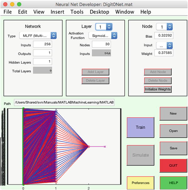
Figure 9.3 A neural net with 256 inputs, one per pixel, an intermediate layer with 30 nodes, and one output.

Our GUI has a separate training window, Figure 9.4. It has buttons for loading and saving training sets, training, and testing the trained neural net. It will plot results automatically based on preferences selected.

Figure 9.4 The Neural Net Training GUI.

9.3.3 How It Works

Then we build the network with 256 inputs, 1 for each pixel; 30 nodes in 1 hidden layer; and 1 output node. We load the training data from the first recipe into the Trainer GUI, and we must select the number of training runs. Two thousand runs should be sufficient if our neuron functions are selected properly. We have an additional parameter to select, the learning rate for the backpropagation; it is reasonable to start with a value of 1.0. Note that our training data script assigned 75% of the images for training and reserved the remainder for testing, using randperm to extract a random set of images. The training records the weights and biases for each run and generates plots on completion. We can easily plot these for the output node, which has just 30 nodes and 1 bias. See Figure 9.5.

Figure 9.5 Layer 2 node weights and biases evolution.

The training function also outputs the training error as the net evolves and the root-mean-square (RMS) of the error.

Figure 9.6 Single-digit training error and RMS error.

Since we have a large number of input neurons, a line plot is not very useful for visualizing the evolution of the weights for the hidden later. However, we can view the weights at any given iteration as an image. Figure 9.7 shows the weights for the network with 30 nodes after training visualized using imagesc. We may wonder if we really need all 30 nodes in the hidden layer, or if we could extract the necessary number of features identifying our chosen digit with fewer. In the image on the right, the weights are shown sorted along the dimension of the input pixels for each node; we can clearly see that only a few nodes seem to have much variation from the random values they are initialized with. That is, many of our nodes seem to be having no impact.

Figure 9.7 Single-digit network, 30-node hidden layer weights. The image on the left shows the weight value. The image on the rights shows the weights sorted by pixel for each node.

Since this visualization seems helpful, we add the code to the training GUI after the generation of the weights line plots. We create two images in one figure, the initial value of the weights on the left and the training values on the right. The HSV colormap looks more striking here than the default Parula map. The code that generates the images in NeuralNetTrainer looks like this:

% New figure: weights as image

newH = figure(’name’,[’Node␣Weights␣for␣Layer␣’ num2str(j)]);

endWeights = [h.train.network(j,1).w(:);h.train.network(j,end).w(:)];

minW = min(endWeights);

maxW = max(endWeights);

subplot(1,2,1)

imagesc(h.train.network(j,1).w,[minW maxW])

colorbar

ylabel(’Output␣Node’)

xlabel(’Input␣Node’)

title(’Weights␣Before␣Training’)

subplot(1,2,2)

imagesc(h.train.network(j,end).w,[minW maxW])

colorbar

xlabel(’Input␣Node’)

title(’Weights␣After␣Training’)

        colormap hsv

h.resultsFig = [newH; h.resultsFig];

Note that we compute the minimum and maximum weight values among both the initial and final iterations, for scaling the two colormaps the same. Now, since many of our 30 initial nodes seemed unneeded, we reduce the number of nodes in that layer to 10, reinitialize the weights (randomly), and train again. Now we get our new figure with the weights displayed as an image bot before and after the training, Figure 9.8.

Figure 9.8 Single-digit network, 10-node hidden layer weights before and after training. The first figure shows the images for the first layer, and the second for the second layer, which has just one output.

Now we can see more patches of colors that have diverged from the initial random weights in the images for the 256 pixel weights, and we see clear variation in the weights for the second layer as well.

9.4.1 Problem

We want to test the neural net.

9.4.2 Solution

We can test the network with inputs that were not used in training. This is explicitly allowed in the GUI as it has separate indices for the training data and testing data. We selected 150 of our sample images for training and saved the remaining 50 for testing in our DigitTrainingData script.

9.4.3 How It Works

In the case of our GUI, simply click the test button to run the neural network with each of the cases selected for training.

Figure 9.9 shows the results for a network with the output node using the sigmoid magnitude function and another case with the output node using a step function; that is, the output is limited to 0 or 1.

Figure 9.9 Neural net results with sigmoid (left) and step (right) activation functions.

The GUI allows you to save the trained net for future use.

9.5.1 Problem

We want to build a neural net that can detect all 10 digits separately.

9.5.2 Solution

Add nodes so that the output layer has 10 nodes, each of which will be 0 or 1 when the representative digit (0–9) is input. Try the output nodes with different functions, like logistic and step. Now that we have more digits, we will go back to having 30 nodes in the hidden layer.

9.5.3 How It Works

Our training data now consist of all 10 digits, with a binary output of zeros with a 1 in the correct slot. For example, a 1 will be represented as [0 1 0 0 0 0 0 0 0]

We follow the same procedure for training. We initialize the net, load the training set into the GUI, and specify the number of training runs for the backpropagation.

The training data, in Figure 9.11, shows that much of the learning is achieved in the first 3000 runs.

Figure 9.10 Net with multiple outputs.

Figure 9.11 Training RMS for multiple-digit neural net.

The test data, in Figure 9.12, show that each set of digits (in sets of 20 in this case, for 200 total tests) is correctly identified.

Figure 9.12 Test results for multiple-digit neural net.

Once you have saved a net that is working well to a MAT-file, you can call it with new data using the function NeuralNetMLFF.

>> data = load(’NeuralNetMat’);

>> network = data.DigitsStepNet;

>> y = NeuralNetMLFF( DigitTrainingTS.inputs(:,1), data.DigitsStepNet )

y =

     1

     0

     0

     0

     0

     0

     0

     0

     0

     0

Again, it is fun to play with visualization of the neural net weights, to gain insight into the problem, and our problem is small enough that we can do so with images. We can view a single set of 256 weights for one hidden neuron as a 16 x 16 image, and view the whole set with each neuron its own row as before (Figure 9.13), to see the patterns emerging.

Figure 9.13 Multiple-digit neural net weights.

You can see parts of digits as mini-patterns in the individual node weights. Simply use imagesc with reshape like this:

>> figure;

>> imagesc(reshape(net.DigitsStepNet.layer(1).w(23,:),16,16));

>> title(’Weights␣to␣Hidden␣Node␣23’)

and see images as in Figure 9.14.

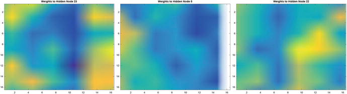
Figure 9.14 Multiple-digit neural net weights.