
Control systems need to react to the environment in a predicable and repeatable fashion. Control systems take measurements and use them to control the process. For example, a ship measures its heading and changes its rudder angle to attain that heading.
Typically, control systems are designed and implemented with all of the parameters hard coded into the software. This works very well in most circumstances, particularly when the system is well known during the design process. When the system is not well defined, or is expected to change significantly during operation, it may be necessary to implement learning control. For example, the batteries in an electric car degrade over time. This leads to less range. An autonomous driving system would need to learn that range was decreasing. This would be done by comparing the distance traveled with the battery state of charge. More drastic, and sudden, changes can alter a system. For example, in an aircraft the air data system might fail due to a sensor malfunction. If the Global Positioning System (GPS) were still operating, the plane would want to switch to a GPS-only system. In a multiinput–multioutput control system, a branch may fail, leaving other branches working fine. The system might have to modify to operating branches in that case.
Learning and adaptive control are often used interchangeably. In this chapter you will learn a variety of techniques for adaptive control for different systems. Each technique is applied to a different system, but all are generally applicable to any control system.
Figure 11.1 provides a taxonomy of adaptive and learning control. The paths depend on the nature of the dynamical system. The rightmost branch is tuning. This is something a designer would do during testing, but it could also be done automatically as will be described in the self-tuning recipe 11.1. The next path is for systems that will vary with time. Our first example is using model reference adaptive control for a spinning wheel. This is discussed in Section 11.2.

Figure 11.1 Taxonomy of adaptive or learning control.
The aircraft section 11.3 is for the longitudinal control of an aircraft that needs to work as the altitude and speed change. You will learn how to implement a neural net to produce the critical parameters for nonlinear control. This is an example of online learning. You have seen examples of neural nets in the chapter on deep learning.
The final example in 11.4 is for ship control. You want to control the heading angle. The dynamics of the ship are a function of the forward speed. This is an example of gain scheduling. While it isn’t really learning from experience, it is adapting based on information about its environment.
11.1 Self-Tuning: Finding the Frequency of an Oscillator
We want to tune a damper so that we critically damp a spring system for which the spring constant changes. Our system will work by perturbing the undamped spring with a step and measuring the frequency using a fast Fourier transform (FFT). We then compute the damping using the frequency and add a damper to the simulation. We then measure the undamped natural frequency again to see that it is the correct value. Finally, we set the damping ratio to 1 and observe the response. The system in shown in Figure 11.2.

Figure 11.2 Spring-mass-damper system. The mass is on the right. The spring is on the top to the left of the mass. The damper is below.
In Chapter 10 we introduced parameter identification, which is another way of finding the frequency. The approach here is to collect a large sample of data and process it in batch to find the natural frequency. The equations for the system are ![]() (11.1)
(11.1)
![]() (11.2)
(11.2)
A dot above the symbols means first derivative with respect to time. That is,  (11.3)
The equations state that the change in position with respect to time is the velocity and the mass times the change in velocity with respect to time is equal to a force proportional to its velocity and position. The second equation is Newton’s law, ![]() (11.4)
(11.4)
where ![]() (11.5)
(11.5)
![]() (11.6)
(11.6)
Our control system generates the component of force − cv.
11.1.1 Problem
We want to identify the frequency of an oscillator.
11.1.2 Solution
The solution is to have the control system adapt to the frequency of the spring. We will use an FFT to identify the frequency of the oscillation.
11.1.3 How It Works
The following script shows how an FFT identifies the oscillation frequency for a damped oscillator.
The function is shown in the following code. We use the RHSOscillator dynamical model for the system. We start with a small initial position to get it to oscillate. We also have a small damping ratio so it will damp out. The resolution of the spectrum is dependent on the number of samples  (11.7)
where n is the number of samples and T is the sampling period. The maximum frequency is ![]() (11.8)
(11.8)
%% Initialize
nSim = 2^16; % Number of time steps
dT = 0.1; % Time step (sec)
dRHS = RHSOscillator; % Get the default data structure
dRHS.omega = 0.1; % Oscillator frequency
dRHS.zeta = 0.1; % Damping ratio
x = [1;0]; % Initial state [position;velocity]
y1Sigma = 0.000; % 1 sigma position measurement noise
%% Simulation
xPlot = zeros(3,nSim);
for k = 1:nSim
% Measurements
y = x(1) + y1Sigma*randn;
% Plot storage
xPlot(:,k) = [x;y];
% Propagate (numerically integrate) the state equations
x = RungeKutta( @RHSOscillator, 0, x, dT, dRHS );
end
%% Plot the results
yL = {’r␣(m)’ ’v␣(m/s)’ ’y_r␣(m)’};
[t,tL] = TimeLabel(dT*(0:(nSim-1)));
PlotSet( t, xPlot, ’x␣label’, tL, ’y␣label’, yL,...
’plot␣title’, ’Oscillator’, ’figure␣title’, ’Oscillator’ );
FFTEnergy( xPlot(3,:), dT );
The FFTEnergy function is shown in the following listing. The FFT takes the sampled time sequence and computes the frequency spectrum. We compute the FFT using MATLAB’s fft function. We take the result and multiply it by its conjugate to get the energy. The first half of the result has the frequency information.
function [e, w, wP] = FFTEnergy( y, tSamp, aPeak )
if( nargin < 3 )
aPeak = 0.95;
end
n = size( y, 2 );
% If the input vector is odd drop one sample
if( 2*floor(n/2) ~= n )
n = n - 1;
y = y(1:n,:);
end
x = fft(y);
e = real(x.*conj(x))/n;
hN = n/2;
e = e(1,1:hN);
r = 2*pi/(n*tSamp);
w = r*(0:(hN-1));
if( nargin > 1 )
k = find( e > aPeak*max(e) );
wP = w(k);
end
if( nargout == 0 )
tL = sprintf(’FFT␣Energy␣Plot:␣Resolution␣=␣%10.2e␣rad/sec’,r);
PlotSet(w,log10(e),’x␣label’,’Frequency␣(rad/sec)’,’y␣label’,’Log
␣␣(Energy)’,’figure␣title’,tL,’plot␣title’,tL,’plot␣type’,’xlog’);
end
Figure 11.3 shows the damped oscillation. Figure 11.4 shows the spectrum. We find the peak by searching for the maximum value. The noise in the signal is seen at the higher frequencies. A noise-free simulation is shown in Figure 11.5.

Figure 11.3 Simulation of the damped oscillator.

Figure 11.4 The frequency spectrum. The peak is at the oscillation frequency of 0.1 rad/s.
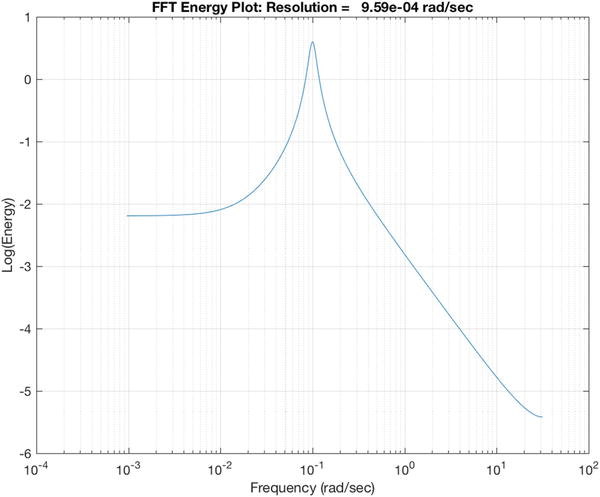
Figure 11.5 The frequency spectrum without noise.
The tuning approach is to
Excite the oscillator with a pulse.
Run it for 2 n steps.
Do an FFT.
If there is only one peak, compute the damping gain.
The script is shown below. It calls FFTEnergy.m with aPeak set to 0.7. The disturbances are Gaussian-distributed accelerations and there is noise in the measurement.
n = 4; % Number of measurement sequences
nSim = 2^16; % Number of time steps
dT = 0.1; % Time step (sec)
dRHS = RHSOscillatorControl; % Get the default data structure
dRHS.omega = 0.1; % Oscillator frequency
zeta = 0.5; % Damping ratio
x = [0;0]; % Initial state [position;velocity]
y1Sigma = 0.001; % 1 sigma position measurement noise
a = 1; % Perturbation
kPulseStop = 10;
aPeak = 0.7;
a1Sigma = 0.01;
%% Simulation
xPlot = zeros(3,n*nSim);
yFFT = zeros(1,nSim);
i = 0;
tuned = false;
wOsc = 0;
for j = 1:n
aJ = a;
for k = 1:nSim
i = i + 1;
% Measurements
y = x(1) + y1Sigma*randn;
% Plot storage
xPlot(:,i) = [x;y];
yFFT(k) = y;
dRHS.a = aJ + a1Sigma*randn;
if( k == kPulseStop )
aJ = 0;
end
% Propagate (numerically integrate) the state equations
x = RungeKutta( @RHSOscillatorControl, 0, x, dT, dRHS );
end
FFTEnergy( yFFT, dT );
[~, ~, wP] = FFTEnergy( yFFT, dT, aPeak );
if( length(wP) == 1 )
wOsc = wP;
fprintf(1,’Estimated␣oscillator␣frequency␣%12.4f␣rad/s ’,wP);
dRHS.c = 2*zeta*wOsc;
else
fprintf(1,’Tuned ’);
end
end
%% Plot the results
yL = {’r␣(m)’ ’v␣(m/s)’ ’y_r␣(m)’};
[t,tL] = TimeLabel(dT*(0:(n*nSim-1)));
PlotSet( t, xPlot, ’x␣label’, tL, ’y␣label’, yL,...
’plot␣title’, ’Oscillator’, ’figure␣title’, ’Oscillator’ );
The results in the command window are
TuningSim
Estimated oscillator frequency 0.0997 rad/s
Tuned
Tuned
Tuned
This is a crude approach. As you can see from the FFT plots, the spectra are “noisy” due to the sensor noise and Gaussian disturbance. The criterion for determining that it is underdamped is that it is a distinctive peak. If the noise is large enough, we have to set lower thresholds.
An important point is that we must stimulate the system to identify the peak. All system identification, parameter estimation, and tuning algorithms have this requirement. An alternative to a pulse (which has a broad frequency spectrum) would be to use a sinusoidal sweep. That would excite any resonances and make it easier to identify the peak.

Figure 11.6 Tuning simulation results. The first four plots are the frequency spectrums taken at the end of each sampling interval; the last shows the results over time.
11.2 Model Reference Adaptive Control
We want to control a robot with an unknown load so that it behaves in a desired manner. The dynamical model of the robot joint is [1]  (11.9)
where the damping a and/or input constants b are unknown. u is the input voltage and u
d
is a disturbance angular acceleration. This is a first-order system. We would like the system to behave like the reference model

Figure 11.7 Speed control of a robot for the model reference adaptive control demo.
 (11.10)
11.2.1 Generating a Square Wave Input
Problem We need to generate a square wave to stimulate the rotor. Solution For the purposes of simulation and testing our controller, we will generate a square wave with a MATLAB function.
How It Works The following function generates a square wave SquareWave.
function [v,d] = SquareWave( t, d )
if( nargin < 1 )
if( nargout == 0 )
Demo;
else
v = DataStructure;
end
return
end
if( d.state == 0 )
if( t - d.tSwitch >= d.tLow )
v = 1;
d.tSwitch = t;
d.state = 1;
else
v = 0;
end
else
if( t - d.tSwitch >= d.tHigh )
v = 0;
d.tSwitch = t;
d.state = 0;
else
v = 1;
end
end
function d = DataStructure
%% Default data structure
d = struct();
d.tLow = 10.0;
d.tHigh = 10.0;
d.tSwitch = 0;
d.state = 0;
function Demo
%% Demo
d = SquareWave;
t = linspace(0,100,1000);
v = zeros(1,length(t));
for k = 1:length(t)
[v(k),d] = SquareWave(t(k),d);
end
PlotSet(t,v,’x␣label’, ’t␣(sec)’, ’y␣label’, ’v’, ’plot␣title’,’Square␣Wave’,... ’figure␣title’, ’Square␣Wave’);
A square wave is shown in Figure 11.8. There are many ways to specify a square wave. This function produces a square wave with a minimum of zero and maximum of 1. You specify the time at zero and the time at 1 to create the square wave.

Figure 11.8 Square wave.
11.2.2 Implement Model Reference Adaptive Control
11.2.2.1 Problem
We want to control a system to behave like a particular model.
11.2.2.2 Solution
The solution is to implement model reference adaptive control (MRAC).
11.2.2.3 How It Works
Hence, the name model reference adaptive control. We will use the MIT rule to design the adaptation system. The MIT rule was first developed at the MIT Instrumentation Laboratory (now Draper Laboratory) that developed the Apollo and Shuttle guidance and control systems.
Consider a closed-loop system with one adjustable parameter, θ. The desired output is y
m
. Let ![]() (11.11)
(11.11)
Define a loss function (or cost) as  (11.12)
The square removes the sign. If the error is zero, the cost is zero. We would like to minimize J(θ). To make J small we change the parameters in the direction of the negative gradient of J or  (11.13)
This is the MIT rule. This can be applied when there is more than one parameter. If the system is changing slowly, then we can assume that θ is constant as the system adapts.
Let the controller be ![]() (11.14)
(11.14)
The second term provides the damping. The controller has two parameters. If they are ![]() (11.15)
(11.15)
![]() (11.16)
(11.16)
the error is ![]() (11.17)
(11.17)
With the parameters θ
1 and θ
2 the system is  (11.18)
To continue with the implementation we introduce the operator ![]() . Set u
d
= 0. We then write
. Set u
d
= 0. We then write ![]() (11.19)
(11.19)
or  (11.20)
We need to get the partial derivatives of the error with respect to θ
1 and θ
2. These are ![]() (11.21)
(11.21)
![]() (11.22)
(11.22)
from the chain rule for differentiation. Noting that  (11.23)
the second equation becomes ![]() (11.24)
(11.24)
Since we don’t know a, let’s assume that we are pretty close to it. Then let ![]() (11.25)
(11.25)
Our adaptation laws are now ![]() (11.26)
(11.26)
![]() (11.27)
(11.27)
where γ is the adaptation gain. The terms in the parentheses are two differential equations, so the complete set is ![]() (11.28)
(11.28)
![]() (11.29)
(11.29)
![]() (11.30)
(11.30)
![]() (11.31)
(11.31)
![]() (11.32)
(11.32)
As noted before, the controller is ![]() (11.33)
(11.33)
![]() (11.34)
(11.34)
![]() (11.35)
(11.35)
The MRAC is implemented in the function MRAC. The controller has five differential equations that are propagated. RungeKutta is used for the propagation, but a less computationally intensive lower-order integrator, such as Euler, could be used instead.
function d = MRAC( omega, d )
if( nargin < 1 )
d = DataStructure;
return
end
d.x = RungeKutta( @RHS, 0, d.x, d.dT, d, omega );
d.u = d.x(3)*d.uC - d.x(4)*omega;
function d = DataStructure
%% Default data structure
d = struct();
d.aM = 2.0;
d.bM = 2.0;
d.x = [0;0;0;0;0];
d.uC = 0;
d.u = 0;
d.gamma = 1;
d.dT = 0.1;
function xDot = RHS( ~, x, d, omega )
%% RHS for MRAC
e = omega - x(5);
xDot = [-d.aM*x(1) + d.aM*d.uC;...
-d.aM*x(2) + d.aM*omega;...
-d.gamma*x(1)*e;...
d.gamma*x(2)*e;...
-d.aM*x(5) + d.bM*d.uC];
11.2.3 Demonstrate MRAC for a Rotor
11.2.3.1 Problem
We want to control our rotor using MRAC.
11.2.3.2 Solution
The solution is to implement MRAC in a MATLAB script.
11.2.3.3 How It Works
MRAC is implemented in the script RotorSim. It calls MRAC to control the rotor. As in our other scripts, we use PlotSet. Notice that we use two new options. One ’plot set’ allows you to put more than one line on a subplot. The other ’legend’ adds legends to each plot. The cell array argument to ’legend’ has a cell array for each plot. In this case we have two plots each with two lines, so the cell array is
{{’true’ ’estimated’} {’Control’ ’Command’}}
Each plot legend is a cell entry within the overall cell array.
The rotor simulation script with MRAC is shown in the following listing. The square wave function generates the command to the system that ω should track. RHSRotor, SquareWave and MRAC all return default data structures.
%% Initialize
nSim = 4000; % Number of time steps
dT = 0.1; % Time step (sec)
dRHS = RHSRotor; % Get the default data structure
dC = MRAC;
dS = SquareWave;
x = 0.1; % Initial state vector
%% Simulation
xPlot = zeros(4,nSim);
theta = zeros(2,nSim);
t = 0;
for k = 1:nSim
% Plot storage
xPlot(:,k) = [x;dC.x(5);dC.u;dC.uC];
theta(:,k) = dC.x(3:4);
[uC, dS] = SquareWave( t, dS );
dC.uC = 2*(uC - 0.5);
dC = MRAC( x, dC );
dRHS.u = dC.u;
% Propagate (numerically integrate) the state equations
x = RungeKutta( @RHSRotor, t, x, dT, dRHS );
t = t + dT;
end
%% Plot the results
yL = {’omega␣(rad/s)’ ’u’};
[t,tL] = TimeLabel(dT*(0:(nSim-1)));
h = PlotSet( t, xPlot, ’x␣label’, tL, ’y␣label’, yL,’plot␣title’, {’Angular␣Rate’ ’Control’},... ’figure␣title’, ’Rotor’, ’plot␣set’,{[1 2] [3 4]},’legend’,{{’true’ ’estimated’} {’Control’ ’Command’}} );
PlotSet( theta(1,:), theta(2,:), ’x␣label’, ’ heta_1’,...
’y␣label’,’ heta_2’, ’plot␣title’, ’Controller␣Parameters’,...
’figure␣title’, ’Controller␣Parameters’ );
The results are shown in Figure 11.9. We set the adaptation gain γ to 1. a
m
and b
m
are set equal to 2. a is set equal to 1 and b to ![]() .
.

Figure 11.9 MRAC control of a first-order system.
The first plot shows the angular rate of the rotor and the control demand and actual control sent to the wheel. The desired control is a square wave (generated by SquareWave). Notice the transient in the applied control at the transitions of the square wave. The control amplitude is greater than the commanded control. Notice also that the angular rate approaches the desired commanded square wave shape.
Figure 11.10 shows the convergence of the adaptive gains, θ 1 and θ 2. They have converged by the end of the simulation.

Figure 11.10 Gain convergence in the MRAC controller.
MRAC learns the gains of the system by observing the response to the control excitation. It requires excitation to converge. This is the nature of all learning systems. If there is no stimulation, it isn’t possible to observe the behavior of the system so that the system can learn. It is easy to find an excitation for a first-order system. For higher-order systems, or nonlinear systems, this is more difficult.
11.3 Longitudinal Control of an Aircraft
In this section we are going to control the longitudinal dynamics of an aircraft using learning control. We will derive a simple longitudinal dynamics model with a “small” number of parameters. Our control will use nonlinear dynamics inversion with a proportional–integral–derivative (PID) controller to control the pitch dynamics. Learning will be done using a sigma-pi neural network.
We will use the learning approach developed at NASA Dryden Research Center [4]. The baseline controller is a dynamic inversion-type controller with a PID control law. A neutral net [3] provides learning while the aircraft is operating. The neutral network is a sigma-pi–type network, meaning that the network sums the products of the inputs with their associated weights. The weights of the neural network are determined by a training algorithm that uses
Commanded aircraft rates from the reference model
PID errors and
Adaptive control rates fed back from the neural network
11.3.1 Write the Differential Equations for the LongitudinalMotion of an Aircraft
11.3.1.1 Problem
We want to model the longitudinal dynamics of an aircraft.
11.3.1.2 Solution
The solution is to write the right-hand-side function for the aircraft longitudinal dynamics differential equations.
11.3.1.3 How It Works
The longitudinal dynamics of an aircraft are also known as the pitch dynamics. The dynamics are entirely in the plane of symmetry of the aircraft. These dynamics include the forward and version motion of the aircraft and the pitching of the aircraft about the axis perpendicular to the plane of symmetry. Figure 11.11 shows an aircraft in flight. α is the angle of attack, the angle between the wing and the velocity vector. We assume that the wind direction is opposite that of the velocity vector; that is, the aircraft produces all of its wind. Drag is along the wind direction and lift is perpendicular to drag. The pitch moment is around the center of mass. The model we will derive uses a small set of parameters yet reproduces the longitudinal dynamics reasonably well. It is also easy for you to modify to simulate any aircraft of interest. We summarized the symbols for the dynamical model in Table 11.1. Our aerodynamic model is very simple. The lift and drag are

Figure 11.11 Diagram of an aircraft in flight showing all the important quantities for longitudinal dynamics simulation.
Table 11.1 Aircraft Dynamics Symbols
Symbol | Description | Units |
|---|---|---|
g | Acceleration of gravity at sea level | 9.806 m/s2 |
h | Altitude | m |
k | Coefficient of lift-induced drag | |
m | Mass | kg |
p | Dynamic pressure | N/m2 |
q | Pitch angular rate | rad/s |
u | x-velocity | m/s |
w | z-velocity | m/s |
C L | Lift coefficient | |
C D | Drag coefficient | |
D | Drag | N |
I y | Pitch moment of inertia | kg-m2 |
L | Lift | N |
M | Pitch moment (torque) | Nm |
M e | Pitch moment due to elevator | Nm |
r e | Elevator moment arm | m |
S | Wetted area of wings | m2 |
S e | Wetted area of elevator | m2 |
T | Thrust | N |
X | X force in the aircraft frame | N |
Z | Z force in the aircraft frame | N |
α | Angle of attack | rad |
γ | Flight path angle | rad |
ρ | Air density | kg/m3 |
θ | Pitch angle | rad |
![]() (11.36)
(11.36)
![]() (11.37)
(11.37)
where S is the wetted area, or the area that is counted in computing the aerodynamic forces, and p is the dynamic pressure, the pressure on the aircraft caused by its velocity,  (11.38)
where ρ is the atmospheric density and v is the magnitude of the velocity. Atmospheric density is a function of altitude. S is the wetted area, that is, the area of the aircraft that interacts with the airflow. For low-speed flight, this is mostly the wings. Most books use q for dynamic pressure. We use q for pitch angular rate (also a convention), so we use p here to avoid confusion.
The lift coefficient, C
L
, is ![]() (11.39)
(11.39)
and the drag coefficient, C
D
, is ![]() (11.40)
(11.40)
The drag equation is called the drag polar. Increasing the angle of attack increases the aircraft lift but also increases the aircraft drag. The coefficient k is  (11.41)
where ε
0 is the Oswald efficiency factor that is typically between 0.75 and 0.85. AR is the wing aspect ratio. The aspect ratio is the ratio of the span of the wing to its chord. For complex shapes it is approximately given by the formula  (11.42)
where b is the span and S is the wing area. Span is measured from wingtip to wingtip. Gliders have very high aspect ratios and delta-wing aircraft have low aspect ratios.
The aerodynamic coefficients are nondimensional coefficients that when multiplied by the wetted area of the aircraft, and the dynamic pressure, produce the aerodynamic forces.
The dynamical equations, the differential equations of motion, are [2] ![]() (11.43)
(11.43)
![]() (11.44)
(11.44)
![]() (11.45)
(11.45)
![]() (11.46)
(11.46)
m is the mass, u is the x-velocity, w is the z-velocity, q is the pitch angular rate, θ is the pitch angle, T is the engine thrust, ε is the angle between the thrust vector and the x-axis, I
y
is the pitch inertia, X is the x-force, Z is the z-force, and M is the torque about the pitch axis. The coupling between x- and z-velocities is caused by writing the force equations in the rotating frame. The pitch equation is about the center of mass. These are a function of u, w, q and altitude, h, which is found from ![]() (11.47)
(11.47)
The angle of attack, α, is the angle between the u- and w-velocities and is ![]() (11.48)
(11.48)
The flight path angle γ is the angle between the vector velocity direction and the horizontal. It is related to θ and α by the relationship ![]() (11.49)
(11.49)
This does not appear in the equations, but it is useful to compute when studying aircraft motion. The forces are ![]() (11.50)
(11.50)
![]() (11.51)
(11.51)
The moment, or torque, is assumed due to the offset of the center of pressure and center of mass, which is assumed to be along the x-axis. ![]() (11.52)
(11.52)
where c
p
is the location of the center of pressure. The moment from the elevator is ![]() (11.53)
(11.53)
S
e
is the wetted area of the elevator and r
E
is the distance from the center of mass to the elevator. The dynamical model is in RHSAircraft. The atmospheric density model is an exponential model and is included as a subfunction in this function.
function [xDot, lift, drag, pD] = RHSAircraft( ~, x, d )
if( nargin < 1 )
xDot = DataStructure;
return
end
g = 9.806;
u = x(1);
w = x(2);
q = x(3);
theta = x(4);
h = x(5);
rho = AtmDensity( h );
alpha = atan(w/u);
cA = cos(alpha);
sA = sin(alpha);
v = sqrt(u^2 + w^2);
pD = 0.5*rho*v^2; % Dynamic pressure
cL = d.cLAlpha*alpha;
cD = d.cD0 + d.k*cL^2;
drag = pD*d.s*cD;
lift = pD*d.s*cL;
x = lift*sA - drag*cA;
z = -lift*cA - drag*sA;
m = d.c*z + pD*d.sE*d.rE*sin(d.delta);
sT = sin(theta);
cT = cos(theta);
tEng = d.thrust*d.throttle;
cE = cos(d.epsilon);
sE = sin(d.epsilon);
uDot = (x + tEng*cE)/d.mass - q*w - g*sT + d.externalAccel(1);
wDot = (z - tEng*sE)/d.mass + q*u + g*cT + d.externalAccel(2);
qDot = m/d.inertia + d.externalAccel(3);
hDot = u*sT - w*cT;
xDot = [uDot;wDot;qDot;q;hDot];
function d = DataStructure
%% Data structure
% F-16
d = struct();
d.cLAlpha = 2*pi; % Lift coefficient
d.cD0 = 0.0175; % Zero lift drag coefficient
d.k = 1/(pi*0.8*3.09); % Lift coupling coefficient A/R 3.09, Oswald Efficiency Factor 0.8
d.epsilon = 0; % rad
d.thrust = 76.3e3; % N
d.throttle = 1;
d.s = 27.87; % wing area m^2
d.mass = 12000; % kg
d.inertia = 1.7295e5; % kg-m^2
d.c = 2; % m
d.sE = 25; % m^2
We will use a model of the F-16 aircraft for our simulation. The F-16 is a single-engine supersonic multirole combat aircraft used by many countries. The F-16 is shown in Figure 11.12.

Figure 11.12 F-16 model.
The inertia matrix is found by taking this model, distributing the mass among all the vertices, and computing the inertia from the formulas ![]() (11.54)
(11.54)
![]() (11.55)
(11.55)
![]() (11.56)
(11.56)
where N is the number of nodes and r
k
is the vector from the origin (which is arbitrary) to node k.
inr =
1.0e+05 *
0.3672 0.0002 -0.0604
0.0002 1.4778 0.0000
-0.0604 0.0000 1.7295
The F-16 data are given in Table 11.2.
Table 11.2 F-16 data.
Symbol | Field | Value | Description | Units |
|---|---|---|---|---|
| cLAlpha | 6.28 | Lift coefficient | |
| cD0 | 0.0175 | Zero lift drag coefficient | |
k | k | 0.1288 | Lift coupling coefficient | |
ε | epsilon | 0 | Thrust angle from the x-axis | rad |
T | thrust | 76.3e3 | Engine thrust | N |
S | s | 27.87 | Wing area | m2 |
m | mass | 12000 | Aircraft mass | kg |
I y | inertia | 1.7295e5 | z-axis inertia | kg-m2 |
c − c p | c | 1 | Offset of center of mass from the center of pressure | m |
S e | sE | 3.5 | Elevator area | m2 |
r e | (rE) | 4.0 | Elevator moment arm | m |
There are many limitations to this model. First of all, the thrust is applied immediately with 100% accuracy. The thrust is also not a function of airspeed or altitude. Real engines take some time to achieve the commanded thrust and the thrust levels change with airspeed and altitude. The elevator also responds instantaneously. Elevators are driven by motors, usually hydraulic but sometimes pure electric, and they take time to reach a commanded angle. The aerodynamics are very simple. Lift and drag are complex functions of airspeed and angle of attack. Usually they are modeled with large tables of coefficients. We also model the pitching moment by a moment arm. Usually the torque is modeled by a table. No aerodynamic damping is modeled though this appears in most complete aerodynamic models for aircraft. You can easily add these features by creating functions
C_L = CL(v,h,alpha,delta)
C_D = CD(v,h,alpha,delta)
C_M = CL(v,h,vdot,alpha,delta)
11.3.2 Numerically Finding Equilibrium
11.3.2.1 Problem
We want to determine the equilibrium state for the aircraft.
11.3.2.2 Solution
The solution is to compute the Jacobian for the dynamics.
11.3.2.3 How It Works
We want to start every simulation from an equilibrium state. This is done using the function EquilibriumState. It uses fminsearch to minimize ![]() (11.57) given the flight speed, altitude, and flight path angle. It then computes the elevator angle needed to zero the pitch angular acceleration. It has a built-in demo for equilibrium-level flight at 10 km.
(11.57) given the flight speed, altitude, and flight path angle. It then computes the elevator angle needed to zero the pitch angular acceleration. It has a built-in demo for equilibrium-level flight at 10 km.
%% Code
if( nargin < 1 )
Demo;
return
end
x = [v;0;0;0;h];
[~,~,drag] = RHSAircraft( 0, x, d );
y0 = [0;drag];
cost(1) = RHS( y0, d, gamma, v, h );
y = fminsearch( @RHS, y0, [], d, gamma, v, h );
w = y(1);
thrust = y(2);
u = sqrt(v^2-w^2);
alpha = atan(w/u);
theta = gamma + alpha;
cost(2) = RHS( y, d, gamma, v, h );
x = [u;w;0;theta;h];
d.thrust = thrust;
d.delta = 0;
[xDot,~,~,p] = RHSAircraft( 0, x, d );
delta = -asin(d.inertia*xDot(3)/(d.rE*d.sE*p));
d.delta = delta;
radToDeg = 180/pi;
fprintf(1,’Velocity␣␣␣␣␣␣␣␣␣␣%8.2f␣m/s ’,v);
fprintf(1,’Altitude␣␣␣␣␣␣␣␣␣␣%8.2f␣m ’,h);
fprintf(1,’Flight␣path␣angle␣%8.2f␣deg ’,gamma*radToDeg);
fprintf(1,’Z␣speed␣␣␣␣␣␣␣␣␣␣␣%8.2f␣m/s ’,w);
fprintf(1,’Thrust␣␣␣␣␣␣␣␣␣␣␣␣%8.2f␣N ’,y(2));
fprintf(1,’Angle␣of␣attack␣␣␣%8.2f␣deg ’,alpha*radToDeg);
fprintf(1,’Elevator␣␣␣␣␣␣␣␣␣␣%8.2f␣deg ’,delta*radToDeg);
fprintf(1,’Initial␣cost␣␣␣␣␣␣%8.2e ’,cost(1));
fprintf(1,’Final␣cost␣␣␣␣␣␣␣␣%8.2e ’,cost(2));
function cost = RHS( y, d, gamma, v, h )
%% Cost function for fminsearch
w = y(1);
d.thrust = y(2);
d.delta = 0;
u = sqrt(v^2-w^2);
alpha = atan(w/u);
theta = gamma + alpha;
x = [u;w;0;theta;h];
xDot = RHSAircraft( 0, x, d );
cost = xDot(1:2)’*xDot(1:2);
function Demo
%% Demo
d = RHSAircraft;
gamma = 0.0;
v = 250;
The results of the demo are
>> EquilibriumState
Velocity 250.00 m/s
Altitude 10000.00 m
Flight path angle 0.00 deg
Z speed 13.84 m/s
Thrust 11148.95 N
Angle of attack 3.17 deg
Elevator -11.22 deg
Initial cost 9.62e+01
Final cost 1.17e-17
The initial and final costs show how successful fminsearch was in achieving the objective of minimizing the w and u accelerations.
11.3.3 Numerical Simulation of the Aircraft
11.3.3.1 Problem
We want to simulate the aircraft.
11.3.3.2 Solution
The solution is to create a script that calls the right-hand side in a loop and plots the results.
11.3.3.3 How It Works
The simulation script is shown below. It computes the equilibrium state and then simulates the dynamics in a loop by calling RungeKutta. It then uses PlotSet to plot the results.
%% Initialize
nSim = 2000; % Number of time steps
dT = 0.1; % Time step (sec)
dRHS = RHSAircraft; % Get the default data structure has F-16 data
h = 10000;
gamma = 0.0;
v = 250;
nPulse = 10;
[x, dRHS.thrust, dRHS.delta, cost] = EquilibriumState( gamma, v, h, dRHS );
fprintf(1,’Finding␣Equilibrium:␣Starting␣Cost␣%12.4e␣Final␣Cost␣%12.4e ’,cost);
accel = [0.0;0.1;0.0];
%% Simulation
xPlot = zeros(length(x)+2,nSim);
for k = 1:nSim
% Plot storage
[~,L,D] = RHSAircraft( 0, x, dRHS );
xPlot(:,k) = [x;L;D];
% Propagate (numerically integrate) the state equations
if( k > nPulse )
dRHS.externalAccel = [0;0;0];
else
dRHS.externalAccel = accel;
end
x = RungeKutta( @RHSAircraft, 0, x, dT, dRHS );
if( x(5) <= 0 )
break;
end
end
xPlot = xPlot(:,1:k);
%% Plot the results
yL = {’u␣(m/s)’ ’w␣(m/s)’ ’q␣(rad/s)’ ’ heta␣(rad)’ ’h␣(m)’ ’L␣(N)’ ’D␣(N)’};
[t,tL] = TimeLabel(dT*(0:(k-1)));
PlotSet( t, xPlot(1:5,:), ’x␣label’, tL, ’y␣label’, yL(1:5),...
This simulation puts the aircraft into a slight climb.
>> AircraftSimOpenLoop
Velocity 250.00 m/s
Altitude 10000.00 m
Flight path angle 0.57 deg
Z speed 13.83 m/s
Thrust 12321.13 N
Angle of attack 3.17 deg
Elevator 11.22 deg
Initial cost 9.62e+01
Final cost 5.66e-17
Finding Equilibrium: Starting Cost 9.6158e+01 Final Cost 5.6645e-17
The simulation results are shown in Figure 11.13. The aircraft climbs steadily. Two oscillations are seen: a high-frequency one primarily associated with pitch and a low-frequency one with the velocity of the aircraft.
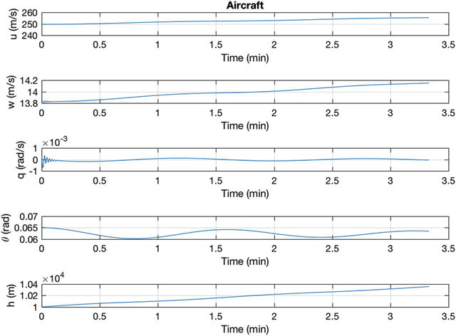
Figure 11.13 Open-loop response to a pulse for the F-16 in a shallow climb.
11.3.4 Find a Limiting and Scaling function for a Neural Net
11.3.4.1 Problem
You need a function to scale and limit measurements.
11.3.4.2 Solution
Use a sigmoid function.
11.3.4.3 How It Works
The neural net uses the following sigmoid function:  (11.58)
The sigmoid function with k = 1 is plotted in the following script.
%% Initialize
x = linspace(-7,7);
%% Sigmoid
s = (1-exp(-x))./(1+exp(-x));
PlotSet( x, s, ’x␣label’, ’x’, ’y␣label’, ’s’,...
’plot␣title’, ’Sigmoid’, ’figure␣title’, ’Sigmoid’ );
Results are shown in Figure 11.14.

Figure 11.14 Sigmoid function. At large values of x, the sigmoid function returns ± 1.
11.3.5 Find a Neural Net for the Learning Control
11.3.5.1 Problem
We need a neural net to add learning to the aircraft control system.
11.3.5.2 Solution
Use a sigma-pi function.
11.3.5.3 How It Works
The adaptive neural network for the pitch axis has seven inputs. The output of the neural network is a pitch angular acceleration that augments the control signal coming from dynamic inversion controller. The control system is shown in Figure 11.15.

Figure 11.15 Aircraft control.
The sigma-pi neutral net is shown in Figure 11.16 for a two-input system.

Figure 11.16 Sigma-pi neural net. Π stands for product and Σ stands for sum.
The output is ![]() (11.59)
(11.59)
The weights are selected to represent the nonlinear function. For example, suppose we want to represent the dynamic pressure  (11.60)
We let x
1 = ρ and x
2 = v
2. Set ![]() and all other weights to zero. Suppose we didn’t know the constant
and all other weights to zero. Suppose we didn’t know the constant ![]() . We would like our neural net to determine the weight through measurements.
. We would like our neural net to determine the weight through measurements.
Learning for a neural net means determining the weights so that our net replicates the function it is modeling. Define the vector z, which is the result of the product operations. In our two-input case this would be  (11.61)
x
1 and x
2 are after the sigmoid operation. The output is ![]() (11.62)
(11.62)
We could assemble multiple inputs and outputs ![]() (11.63)
(11.63)
where z
k
is a column array. We can solve for w using least squares. Define the vector of y to be Y and the matrix of z to be Z. The solution for w is ![]() (11.64)
(11.64)
The least-squares solution is ![]() (11.65)
(11.65)
This gives the best fit to w for the measurements Y and inputs Z. Suppose we take another measurement. We would then repeat this with bigger matrices. Clearly, this is impractical. As a side note you would really compute this using an inverse. There are better numerical methods for doing least squares. MATLAB has the pinv function. For example,
>> z = rand(4,4);
>> w = rand(4,1);
>> y = w’*z;
>> wL = inv(z*z’)*z*y’
wL =
0.8308
0.5853
0.5497
0.9172
>> w
w =
0.8308
0.5853
0.5497
0.9172
>> pinv(z’)*y’
ans =
0.8308
0.5853
0.5497
0.9172
As you can see, they all agree! This is a good way to initially train your neural net. Collect as many measurements as you have values of z and compute the weights. Your net is then ready to go.
The recursive approach is to initialize the recursive trainer with n values of z and y. ![]() (11.66)
(11.66)
![]() (11.67)
(11.67)
The recursive learning algorithm is ![]() (11.68)
(11.68)
![]() (11.69)
(11.69)
![]() (11.70) The following script demonstrates recursive learning or training. It starts with an initial estimate based on a four-element training set. It then recursively learns based on new data.
(11.70) The following script demonstrates recursive learning or training. It starts with an initial estimate based on a four-element training set. It then recursively learns based on new data.
w = rand(4,1); % Initial guess
Z = randn(4,4);
Y = Z’*w;
wN = w + 0.1*randn(4,1); % True weights are a little different
n = 300;
zA = randn(4,n); % Random inputs
y = wN’*zA; % 100 new measurements
% Batch training
p = inv(Z*Z’); % Initial value
w = p*Z*Y; % Initial value
%% Recursive learning
dW = zeros(4,n);
for j = 1:n
z = zA(:,j);
p = p - p*(z*z’)*p/(1+z’*p*z);
w = w + p*z*(y(j) - z’*w);
dW(:,j) = w - wN; % Store for plotting
end
%% Plot the results
yL = cell(1,4);
for j = 1:4
yL{j} = sprintf(’\Delta␣W_%d’,j);
end
PlotSet(1:n,dW,’x␣label’,’Sample’,’y␣label’,yL,...
’plot␣title’,’Recursive␣Training’,...
’figure␣title’,’Recursive␣Training’);
Figure 11.17 shows the results. After an initial transient the learning converges. Every time you run this you will get different answers because we initialize with random values.

Figure 11.17 Recursive training or learning. After an initial transient the weights converge quickly.
You will notice that the recursive learning algorithm is identical in form to the conventional Kalman filter given in Section 10.1.4 Our learning algorithm was derived from batch least squares, which is an alternative derivation for the Kalman filter.
11.3.6 Enumerate All Sets of Inputs
11.3.6.1 Problem
We need a function to enumerate all possible sets of combinations.
11.3.6.2 Solution
Write a combination function.
11.3.6.3 How It Works
We hand coded the products of the inputs. For more general code we want to enumerate all sets of inputs. If we have n inputs and want to take them k at a time, the number of sets is  (11.71)
The code to enumerate all sets is in the function Combinations.
%% Demo
if( nargin < 1 )
Combinations(1:4,3)
return
end
%% Special cases
if( k == 1 )
c = r’;
return
elseif( k == length(r) )
c = r;
return
end
%% Recursion
rJ = r(2:end);
c = [];
if( length(rJ) > 1 )
for j = 2:length(r)-k+1
rJ = r(j:end);
nC = NumberOfCombinations(length(rJ),k-1);
cJ = zeros(nC,k);
cJ(:,2:end) = Combinations(rJ,k-1);
cJ(:,1) = r(j-1);
if( ~isempty(c) )
c = [c;cJ];
else
c = cJ;
end
end
else
c = rJ;
end
c = [c;r(end-k+1:end)];
function j = NumberOfCombinations(n,k)
%% Compute the number of combinations
j = factorial(n)/(factorial(n-k)*factorial(k));
This handles two special cases on input and then calls itself recursively for all other cases. Here are some examples:
>> Combinations(1:4,3)
ans =
1 2 3
1 2 4
1 3 4
2 3 4
>> Combinations(1:4,2)
ans =
1 2
1 3
1 4
2 3
2 4
3 4
You can see that if we have 4 inputs and want all possible combinations we end up with 14 total! This indicates a practical limit to a sigma-pi neural network as the number of weights will grow fast as the number of inputs increases.
11.3.7 Write a General Neural Net Function
11.3.7.1 Problem
We need a neural net function for general problems.
11.3.7.2 Solution
Use a sigma-pi function.
11.3.7.3 How It Works
The following code shows how we implement the sigma-pi neural net. SigmaPiNeuralNet has action as its first input. You use this to access the functionality of the function. Actions are
“initialize”: initialize the function
“set constant”: set the constant term
“batch learning”: perform batch learning
“recursive learning”: perform recursive learning
“output”: generate outputs without training
You usually go in order when running the function. Setting the constant is not needed if the default of 1 is fine.
The functionality is distributed among subfunctions called from the switch statement.
% None.
function [y, d] = SigmaPiNeuralNet( action, x, d )
% Demo or default data structure
if( nargin < 1 )
if( nargout == 1)
y = DefaultDataStructure;
else
Demo;
end
return
end
switch lower(action)
case ’initialize’
d = CreateZIndices( x, d );
d.w = zeros(size(d.zI,1)+1,1);
y = [];
case ’set␣constant’
d.c = x;
y = [];
case ’batch␣learning’
[y, d] = BatchLearning( x, d );
case ’recursive␣learning’
[y, d] = RecursiveLearning( x, d );
case ’output’
[y, d] = NNOutput( x, d );
otherwise
error(’%s␣is␣not␣an␣available␣action’,action );
end
function d = CreateZIndices( x, d )
%% Create the indices
n = length(x);
m = 0;
nF = factorial(n);
for k = 1:n
m = m + nF/(factorial(n-k)*factorial(k));
end
d.z = zeros(m,1);
d.zI = cell(m,1);
i = 1;
for k = 1:n
c = Combinations(1:n,k);
for j = 1:size(c,1)
d.zI{i} = c(j,:);
i = i + 1;
end
end
d.nZ = m+1;
function d = CreateZArray( x, d )
%% Create array of products of x
n = length(x);
d.z(1) = d.c;
for k = 1:d.nZ-1
d.z(k+1) = 1;
for j = 1:length(d.zI(k))
d.z(k+1) = d.z(k)*x(d.zI{k}(j));
end
end
function [y, d] = RecursiveLearning( x, d )
%% Recursive Learning
d = CreateZArray( x, d );
z = d.z;
d.p = d.p - d.p*(z*z’)*d.p/(1+z’*d.p*z);
d.w = d.w + d.p*z*(d.y - z’*d.w);
y = z’*d.w;
function [y, d] = NNOutput( x, d )
%% Output without learning
x = SigmoidFun(x,d.kSigmoid);
d = CreateZArray( x, d );
y = d.z’*d.w;
function [y, d] = BatchLearning( x, d )
%% Batch Learning
z = zeros(d.nZ,size(x,2));
x = SigmoidFun(x,d.kSigmoid);
for k = 1:size(x,2)
d = CreateZArray( x(:,k), d );
z(:,k) = d.z;
end
d.p = inv(z*z’);
d.w = (z*z’)z*d.y;
y = z’*d.w;
function d = DefaultDataStructure
%% Default data structure
d = struct();
d.w = [];
d.c = 1; % Constant term
d.zI = {};
d.z = [];
d.kSigmoid = 0.0001;
d.y = [];
The demo shows an example of using the function to model dynamic pressure. Our inputs are the altitude and the square of the velocity. The neutral net will try to fit ![]() (11.72)
(11.72)
to ![]() (11.73)
(11.73)
We get the default data structure. Then we initialize the filter with an empty x. We then get the initial weights by using batch learning. The number of columns of f x should be at least twice the number of inputs. This gives a starting p matrix and initial estimate of weights. We then perform recursive learning. It is important that the field kSigmoid is small enough so that valid inputs are in the linear region of the sigmoid function. Note that this can be an array so that you can use different scalings on different inputs.
%% Sigmoid function
kX = k.*x;
s = (1-exp(-kX))./(1+exp(-kX));
function Demo
%% Demo
x = zeros(2,1);
d = SigmaPiNeuralNet;
[~, d] = SigmaPiNeuralNet( ’initialize’, x, d );
h = linspace(10,10000);
v = linspace(10,400);
v2 = v.^2;
q = 0.5*AtmDensity(h).*v2;
n = 5;
x = [h(1:n);v2(1:n)];
d.y = q(1:n)’;
[y, d] = SigmaPiNeuralNet( ’batch␣learning’, x, d );
fprintf(1,’Batch␣Results #␣␣␣␣␣␣␣␣␣Truth␣␣␣Neural␣Net ’);
for k = 1:length(y)
fprintf(1,’%d:␣%12.2f␣%12.2f ’,k,q(k),y(k));
end
n = length(h);
y = zeros(1,n);
x = [h;v2];
for k = 1:n
d.y = q(k);
[y(k), d] = SigmaPiNeuralNet( ’recursive␣learning’, x(:,k), d );
end
yL = {’q␣(N/m^2)’ ’v␣(m/s)’ ’h␣(m)’};
The batch results are as follows. This is at low altitude.
>> SigmaPiNeuralNet
Batch Results
# Truth Neural Net
1: 61.22 61.17
2: 118.24 118.42
3: 193.12 192.88
4: 285.38 285.52
5: 394.51 394.48
The recursive learning results are shown in Figure 11.18. The results are pretty good over a wide range of altitudes. You could then just use the “update” action during aircraft operation.

Figure 11.18 Recursive training for the dynamic pressure example.
11.3.8 Implement PID Control
11.3.8.1 Problem
We want a PID controller.
11.3.8.2 Solution
Write a function to implement PID control.
11.3.8.3 How It Works
Assume with we have a double integrator driven by a constant input ![]() (11.74)
(11.74)
where  (11.75)
The result is  (11.76)
The simplest control is to add a feedback controller ![]() (11.77)
(11.77)
where K is the forward gain and τ is the damping time constant. Our dynamical equation is now ![]() (11.78)
(11.78)
The damping term will cause the transients to die out. When that happens the second derivative and first derivatives of x are zero and we end up with an offset ![]() (11.79)
(11.79)
This is generally not desirable. You could increase K until the offset were small, but that would mean your actuator would need to produce higher forces or torques. What we have at the moment is a PD controller, or proportional derivative. Let’s add another term to the controller  (11.80)
This is now a PID controller, or proportional–integral–derivative controller. There is now a gain proportional to the integral of x. We add the new controller and then take another derivative to get  (11.81)
Now in steady state ![]() (11.82)
(11.82)
If u is constant, the offset is zero. Let ![]() (11.83)
(11.83)
Then  (11.84)
 (11.85)
where τ
d
is the rate time constant, which is how long the system will take to damp, and τ
i
is how fast the system will integrate out a steady disturbance.
The open-loop transfer function is  (11.86)
where s = j ω and ![]() . The closed-loop transfer function is
. The closed-loop transfer function is ![]() (11.87)
(11.87)
The desired closed-loop transfer function is ![]() (11.88)
(11.88)
or ![]() (11.89)
(11.89)
The parameters are ![]() (11.90)
(11.90)
![]() (11.91)
(11.91)
![]() (11.92)
(11.92)
This is a design for a PID. However, it is not possible to write this in the desired state-space form ![]() (11.93)
(11.93)
![]() (11.94)
(11.94)
because it has a pure differentiator. We need to add a filter to the rate term so that it looks like ![]() (11.95)
(11.95)
instead of s. We aren’t going to derive the constants and will leave it as an exercise for the reader. The code for the PID is in PID.
function [a, b, c, d] = PID( zeta, omega, tauInt, omegaR, tSamp )
% Demo
if( nargin < 1 )
Demo;
return
end
% Input processing
if( nargin < 4 )
omegaR = [];
end
% Default roll-off
if( isempty(omegaR) )
omegaR = 5*omega;
end
% Compute the PID gains
omegaI = 2*pi/tauInt;
c2 = omegaI*omegaR;
c1 = omegaI+omegaR;
b1 = 2*zeta*omega;
b2 = omega^2;
g = c1 + b1;
kI = c2*b2/g;
kP = (c1*b2 + b1.*c2 - kI)/g;
kR = (c1*b1 + c2 + b2 - kP)/g;
% Compute the state space model
a = [0 0;0 -g];
b = [1;g];
c = [kI -kR*g];
It is interesting to evaluate the effect of the integrator. This is shown in Figure 11.19. The code is the demo in PID. Instead of numerically integrating the differential equations, we convert them into sampled time and propagate them. This is handy for linear equations. The double-integrator equations are in the form ![]() (11.96)
(11.96)
![]() (11.97) This is the same form as the PID controller.
(11.97) This is the same form as the PID controller.

Figure 11.19 PID control given a unit input.
% Convert to discrete time
if( nargin > 4 )
[a,b] = CToDZOH(a,b,tSamp);
end
function Demo
%% Demo
% The double integrator plant
dT = 0.1; % s
aP = [0 1;0 0];
bP = [0;1];
[aP, bP] = CToDZOH( aP, bP, dT );
% Design the controller
[a, b, c, d] = PID( 1, 0.1, 100, 0.5, dT );
% Run the simulation
n = 2000;
p = zeros(2,n);
x = [0;0];
xC = [0;0];
for k = 1:n
% PID Controller
y = x(1);
xC = a*xC + b*y;
uC = c*xC + d*y;
p(:,k) = [y;uC];
x = aP*x + bP*(1-uC); % Unit step response
end
It takes about 2 minutes to drive x to zero, which is close to the 100 seconds specified for the integrator.
11.3.9 Demonstrate PID control of Pitch for the Aircraft
11.3.9.1 Problem
We want to control pitch with a PID control.
11.3.9.2 Solution
Write a script to implement the controller with the PID controller and pitch dynamic inversion compensation.
11.3.9.3 How It Works
The PID controller changes the elevator angle to produce a pitch acceleration to rotate the aircraft. In addition, additional elevator movement is needed to compensate for changes in the accelerations due to lift and drag as the aircraft changes its pitch orientation. This is done using the pitch dynamic inversion function. This returns the pitch acceleration that must be compensated for when applying the pitch control.
function qDot = PitchDynamicInversion( x, d )
if( nargin < 1 )
qDot = DataStructure;
return
end
u = x(1);
w = x(2);
h = x(5);
rho = AtmDensity( h );
alpha = atan(w/u);
cA = cos(alpha);
sA = sin(alpha);
v = sqrt(u^2 + w^2);
pD = 0.5*rho*v^2; % Dynamic pressure
cL = d.cLAlpha*alpha;
cD = d.cD0 + d.k*cL^2;
drag = pD*d.s*cD;
lift = pD*d.s*cL;
z = -lift*cA - drag*sA;
m = d.c*z;
qDot = m/d.inertia;
function d = DataStructure
%% Data structure
% F-16
d = struct();
d.cLAlpha = 2*pi; % Lift coefficient
d.cD0 = 0.0175; % Zero lift drag coefficient
d.k = 1/(pi*0.8*3.09); % Lift coupling coefficient A/R 3.09, Oswald Efficiency Factor 0.8
d.s = 27.87; % wing area m^2
d.inertia = 1.7295e5; % kg-m^2
d.c = 2; % m
d.sE = 25; % m^2
d.delta = 0; % rad
d.rE = 4; % m
d.externalAccel = [0;0;0]; % [m/s^2;m/s^2;rad/s^2[
The simulation incorporating the controls is shown below. There is a flag to turn on control and another to turn on the learning control.
% Options for control
addLearning = true;
addControl = true;
%% Initialize the simulation
nSim = 1000; % Number of time steps
dT = 0.1; % Time step (sec)
dRHS = RHSAircraft; % Get the default data structure has F-16 data
h = 10000;
gamma = 0.0;
v = 250;
nPulse = 10;
pitchDesired = 0.2;
dL = load(’PitchNNWeights’);
[x, dRHS.thrust, deltaEq, cost] = EquilibriumState( gamma, v, h, dRHS );
fprintf(1,’Finding␣Equilibrium:␣Starting␣Cost␣%12.4e␣Final␣Cost␣%12.4e ’,cost);
if( addLearning )
temp = load(’DRHSL’);
dRHSL = temp.dRHSL;
temp = load(’DNN’);
dNN = temp.d;
else
temp = load(’DRHSL’);
dRHSL = temp.dRHSL;
end
accel = [0.0;0.0;0.0];
% Design the PID Controller
[aC, bC, cC, dC] = PID( 1, 0.1, 100, 0.5, dT );
dRHS.delta = deltaEq;
xDotEq = RHSAircraft( 0, x, dRHS );
aEq = xDotEq(3);
xC = [0;0];
%% Simulation
xPlot = zeros(length(x)+8,nSim);
for k = 1:nSim
% Control
[~,L,D,pD] = RHSAircraft( 0, x, dRHS );
% Measurement
pitch = x(4);
% PID control
if( addControl )
pitchError = pitch - pitchDesired;
xC = aC*xC + bC*pitchError;
aDI = PitchDynamicInversion( x, dRHSL );
aPID = -(cC*xC + dC*pitchError);
else
pitchError = 0;
aPID = 0;
end
% Learning
if( addLearning )
xNN = [x(4);x(1)^2 + x(2)^2];
aLearning = SigmaPiNeuralNet( ’output’, xNN, dNN );
else
aLearning = 0;
end
if( addControl )
aTotal = aPID - (aDI + aLearning);
% Convert acceleration to elevator angle
gain = dRHS.inertia/(dRHS.rE*dRHS.sE*pD);
dRHS.delta = asin(gain*aTotal);
else
dRHS.delta = deltaEq;
end
% Plot storage
xPlot(:,k) = [x;L;D;aPID;pitchError;dRHS.delta;aPID;aDI;aLearning];
% Propagate (numerically integrate) the state equations
if( k > nPulse )
dRHS.externalAccel = [0;0;0];
else
dRHS.externalAccel = accel;
end
x = RungeKutta( @RHSAircraft, 0, x, dT, dRHS );
% A crash
if( x(5) <= 0 )
break;
end
end
%% Plot the results
xPlot = xPlot(:,1:k);
yL = {’u␣(m/s)’ ’w␣(m/s)’ ’q␣(rad/s)’ ’ heta␣(rad)’ ’h␣(m)’ ’L␣(N)’ ’D␣(N)’ ’a_{PID}␣(rad/s^2)’ ’delta heta␣(rad)’ ’delta␣(rad)’ ...
’a_{PID}’ ’a_{DI}’ ’a_{L}’};
[t,tL] = TimeLabel(dT*(0:(k-1)));
PlotSet( t, xPlot(1:5,:), ’x␣label’, tL, ’y␣label’, yL(1:5),...
’plot␣title’, ’Aircraft’, ’figure␣title’, ’Aircraft␣State’ );
PlotSet( t, xPlot(6:7,:), ’x␣label’, tL, ’y␣label’, yL(6:7),...
’plot␣title’, ’Aircraft’, ’figure␣title’, ’Aircraft␣L␣and␣D’ );
PlotSet( t, xPlot(8:10,:), ’x␣label’, tL, ’y␣label’, yL(8:10),...
’plot␣title’, ’Aircraft’, ’figure␣title’, ’Aircraft␣Control’ );
PlotSet( t, xPlot(11:13,:), ’x␣label’, tL, ’y␣label’, yL(11:13),...
’plot␣title’, ’Aircraft’, ’figure␣title’, ’Control␣Acceleratins’ );
We command a 0.2-radian pitch angle using the PID control. The results are shown in Figure 11.20, Figure 11.21, and Figure 11.22.

Figure 11.20 Aircraft pitch angle change. The aircraft oscillates due to the pitch dynamics.

Figure 11.21 Aircraft pitch angle change. Notice the changes in lift and drag with angle.

Figure 11.22 Aircraft pitch angle change. The PID acceleration is much lower than the pitch inversion acceleration.
The maneuver increases the drag and we don’t adjust the throttle to compensate. This will cause the airspeed to drop. In implementing the controller we neglected to consider coupling between states, but this can be added easily.
11.3.10 Create the Neural Net for the Pitch Dynamics
11.3.10.1 Problem
We want a nonlinear inversion controller with a PID controller and the neural net learning system.
11.3.10.2 Solution
Train the neural net with a script that takes the angle and velocity squared input and computes the pitch acceleration error.
11.3.10.3 How It Works
The following script computes the pitch acceleration for a slightly different set of parameters. It then processes the delta-acceleration. The script passes a range of pitch angles to the function and learns the acceleration. We use the velocity squared as an input because the dynamic pressure is proportional to the dynamic pressure. Thus, a base acceleration (in dRHSL) is for our “a priori” model. dRHS is the measured values. We assume that these are obtained during flight testing.
dRHS = RHSAircraft; % Get the default data structure has F-16
% data
h = 10000;
gamma = 0.0;
v = 250;
% Get the equilibrium state
[x, dRHS.thrust, deltaEq, cost] = EquilibriumState( gamma, v, h, dRHS );
% Angle of attack
alpha = atan(x(2)/x(1));
cA = cos(alpha);
sA = sin(alpha);
% Create the assumed properties
dRHSL = dRHS;
dRHSL.cD0 = 2.2*dRHS.cD0;
dRHSL.k = 1.0*dRHSL.k;
% 2 inputs
xNN = zeros(2,1);
d = SigmaPiNeuralNet;
[~, d] = SigmaPiNeuralNet( ’initialize’, xNN, d );
theta = linspace(0,pi/8);
v = linspace(300,200);
n = length(theta);
aT = zeros(1,n);
aM = zeros(1,n);
for k = 1:n
x(4) = theta(k);
x(1) = cA*v(k);
x(2) = sA*v(k);
aT(k) = PitchDynamicInversion( x, dRHSL );
aM(k) = PitchDynamicInversion( x, dRHS );
end
% The delta pitch acceleration
dA = aM - aT;
% Inputs to the neural net
v2 = v.^2;
xNN = [theta;v2];
% Outputs for training
d.y = dA’;
[aNN, d] = SigmaPiNeuralNet( ’batch␣learning’, xNN, d );
% Save the data for the aircraft simulation
save( ’DRHSL’,’dRHSL’ );
save( ’DNN’, ’d’ );
The resulting weights are saved in a MAT-file for use in AircraftSim. The simulation uses dRHS, but our pitch acceleration model uses dRHSL. The latter is saved in another MAT-file.
>> PitchNeuralNetTraining
Velocity 250.00 m/s
Altitude 10000.00 m
Flight path angle 0.00 deg
Z speed 13.84 m/s
Thrust 11148.95 N
Angle of attack 3.17 deg
Elevator 11.22 deg
Initial cost 9.62e+01
Final cost 1.17e-17
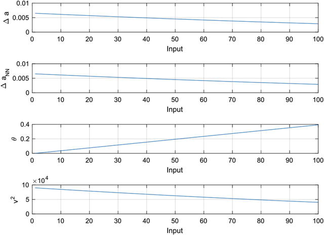
Figure 11.23 Neural net fit to the delta-acceleration
As can be seen, the neural net reproduces the model very well. The script also outputs DNN.mat, which contains the trained neural net data.
11.3.11 Demonstrate the Controller in a Nonlinear Simulation
11.3.11.1 Problem
We want to demonstrate our learning control system.
11.3.11.2 Solution
Enable the control functions to the simulation script described in this chapter.
11.3.11.3 How It Works
After training the neural net in the previous recipe we set addLearning to true. The weights are read in. When learning control is on, it uses the right-hand side. PitchDynamicInversion uses modified parameters that were used in the learning script to compute the weight. This simulates the uncertainty in the models.
We command a 0.2-radian pitch angle using the PID learning control. The results are shown in Figure 11.24, Figure 11.25, and Figure 11.26. The figures show without learning control on the left and with learning control on the right.

Figure 11.24 Aircraft pitch angle change. Lift and drag variations are shown.

Figure 11.25 Aircraft pitch angle change. Without learning control the elevator saturates.
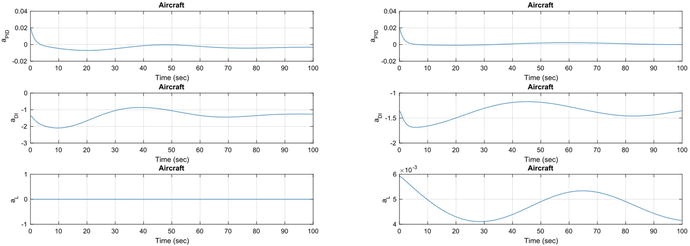
Figure 11.26 Aircraft pitch angle change. The PID acceleration is much lower than the pitch inversion acceleration.
Learning control helps the performance of the controller. However, the weights are fixed throughout the simulation. Learning occurs prior to the controller becoming active. The control system is still sensitive to parameter changes since the learning part of the control was computed for a predetermined trajectory. Our weights were determined only as a function of pitch angle and velocity squared. Additional inputs would improve the performance. There are many opportunities for you to try to expand and improve the learning system.
11.4 Ship Steering: Implement Gain Scheduling for Steering Control of a Ship
11.4.1 Problem
We want to steer a ship at all speeds.
11.4.2 Solution
The solution is to use gain scheduling to set the gains based on speeds. The gain scheduled is learned by automatically computing gains from the dynamical equations of the ship. This is similar to the self-tuning example except that we are seeking a set of gains for all speeds, not just one. In addition, we assume that we know the model of the system.
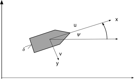
Figure 11.27 Ship heading control for gain scheduling control.
11.4.3 How It Works
The dynamical equations for the heading of a ship are in state-space form [1].  (11.98)
v is the transverse speed, u is the ship’s speed, l is the ship length, r is the turning rate, and ψ is the heading angle. α
v
and α
r
are disturbances. The ship is assumed to be moving at speed u. This is achieved by the propeller that is not modeled. You’ll note we leave out the equation for forward motion. The control is the rudder angle δ. Notice that if u = 0, the ship cannot be steered. All of the coefficients in the state matrix are functions of u, except for the heading angle. Our goal is to control the heading given the disturbance acceleration in the first equation and the disturbance angular rate in the second.
The disturbances only affect the dynamics states, r and v. The last state, ψ, is a kinematic state and does not have a disturbance.
Table 11.3 Ship parameters [1].
Parameter | Minesweeper | Cargo | Tanker |
|---|---|---|---|
l | 55 | 161 | 350 |
a 11 | -0.86 | -0.77 | -0.45 |
a 12 | -0.48 | -0.34 | -0.44 |
a 21 | -5.20 | -3.39 | -4.10 |
a 22 | -2.40 | -1.63 | -0.81 |
b 1 | 0.18 | 0.17 | 0.10 |
b 2 | 1.40 | -1.63 | -0.81 |
The ship model is shown in the following code. The second and third outputs are for use in the controller. Notice that the differential equations are linear in the state and the control. Both matrices are a function of the forward velocity. The default parameters are for the minesweeper in the table.
function [xDot, a, b] = RHSShip( ~, x, d )
if( nargin < 1 )
xDot = struct(’l’,100,’u’,10,’a’,[-0.86 -0.48;-5.2 -2.4],’b’,[0.18;-1.4],’alpha’,[0;0;0],’delta’,0);
return
end
uOL = d.u/d.l;
uOLSq = d.u/d.l^2;
uSqOl = d.u^2/d.l;
a = [ uOL*d.a(1,1) d.u*d.a(1,2) 0;...
uOLSq*d.a(2,1) uOL*d.a(2,2) 0;...
0 1 0];
b = [uSqOl*d.b(1);...
uOL^2*d.b(2);...
0];
xDot = a*x + b*d.delta + d.alpha;
In the ship simulation we linearly increase the forward speed while commanding a series of heading psi changes. The controller takes the state-space model at each time step and computes new gains, which are used to steer the ship. The controller is a linear quadratic regulator. We can use full state feedback because the states are easily modeled. Such controllers will work perfectly in this case but are a bit harder to implement when you need to estimate some of the states or have unmodeled dynamics.
%% Initialize
nSim = 10000; % Number of time steps
dT = 1; % Time step (sec)
dRHS = RHSShip; % Get the default data structure
x = [0;0.001;0.0]; % [lateral velocity;angular velocity;heading]
u = linspace(10,20,nSim)*0.514; % m/s
qC = eye(3); % State cost in the controller
rC = 0.1; % Control cost in the controller
% Desired heading angle
psi = [zeros(1,nSim/4) ones(1,nSim/4) 2*ones(1,nSim/4) zeros(1,nSim/4)];
%% Simulation
xPlot = zeros(3,nSim);
gain = zeros(nSim,3);
delta = zeros(1,nSim);
for k = 1:nSim
% Plot storage
xPlot(:,k) = x;
dRHS.u = u(k);
% Control
% Get the state space matrices
[~,a,b] = RHSShip( 0, x, dRHS );
gain(k,:) = QCR( a, b, qC, rC );
dRHS.delta = -gain(k,:)*[x(1);x(2);x(3) - psi(k)]; % Rudder angle
delta(k) = dRHS.delta;
% Propagate (numerically integrate) the state equations
x = RungeKutta( @RHSShip, 0, x, dT, dRHS );
end
%% Plot the results
yL = {’v␣(m/s)’ ’r␣(rad/s)’ ’psi␣(rad)’ ’u␣(m/s)’ ’Gain␣v’ ’Gain␣r’ ’Gain␣psi’ ’delta␣(rad)’ };
[t,tL] = TimeLabel(dT*(0:(nSim-1)));
PlotSet( t, [xPlot;u], ’x␣label’, tL, ’y␣label’, yL(1:4),...
’plot␣title’, ’Ship’, ’figure␣title’, ’Ship’ );
The quadratic regulator generator code is shown in the following lists. It generates the gain from the matrix Riccati equation. A Riccati equation is an ordinary differential equation that is quadratic in the unknown function. In steady state this reduces to the algebraic Riccati equation that is solved in this function.
function k = QCR( a, b, q, r )
[sinf,rr] = Riccati( [a,-(b/r)*b’;-q’,-a’] );
if( rr == 1 )
disp(’Repeated␣roots.␣Adjust␣q,␣r␣or␣n’);
end
k = r(b’*sinf);
function [sinf, rr] = Riccati( g )
%% Ricatti
% Solves the matrix Riccati equation.
%
% Solves the matrix Riccati equation in the form
%
% g = [a r ]
% [q -a’]
rg = size(g);
[w, e] = eig(g);
es = sort(diag(e));
% Look for repeated roots
j = 1:length(es)-1;
if ( any(abs(es(j)-es(j+1))<eps*abs(es(j)+es(j+1))) ),
rr = 1;
else
rr = 0;
end
% Sort the columns of w
ws = w(:,real(diag(e)) < 0);
sinf = real(ws(rg/2+1:rg,:)/ws(1:rg/2,:));
The results are given in Figure 11.28. Note how the gains evolve.

Figure 11.28 Ship steering simulation. The states are shown on the left with the forward velocity. The gains and rudder angle are shown on the right. Notice the “pulses” in the rudder to make the maneuvers.
The gain on the angular rate r is nearly constant. The other two gains increase with speed. This is an example of gain scheduling. The difference is that we autonomously compute the gains from measurements of the ship’s forward speed.
The next script is a modified version of ShipSim that is a shorter duration, with only one course change, and with disturbances in both angular rate and lateral velocity.
%% Initialize
nSim = 300; % Number of time steps
dT = 1; % Time step (sec)
dRHS = RHSShip; % Get the default data structure
x = [0;0.001;0.0]; % [lateral velocity;angular velocity;heading]
u = linspace(10,20,nSim)*0.514; % m/s
qC = eye(3); % State cost in the controller
rC = 0.1; % Control cost in the controller
alpha = [0.01;0.001]; % 1 sigma disturbances
% Desired heading angle
psi = [zeros(1,nSim/6) ones(1,5*nSim/6)];
%% Simulation
xPlot = zeros(3,nSim);
gain = zeros(nSim,3);
delta = zeros(1,nSim);
for k = 1:nSim
% Plot storage
xPlot(:,k) = x;
dRHS.u = u(k);
% Control
% Get the state space matrices
[~,a,b] = RHSShip( 0, x, dRHS );
gain(k,:) = QCR( a, b, qC, rC );
dRHS.alpha = [alpha.*randn(2,1);0];
dRHS.delta = -gain(k,:)*[x(1);x(2);x(3) - psi(k)]; % Rudder angle
delta(k) = dRHS.delta;
% Propagate (numerically integrate) the state equations
x = RungeKutta( @RHSShip, 0, x, dT, dRHS );
end
%% Plot the results
yL = {’v␣(m/s)’ ’r␣(rad/s)’ ’psi␣(rad)’ ’u␣(m/s)’ ’Gain␣v’ ’Gain␣r’
’Gain␣psi’ ’delta␣(rad)’ };
[t,tL] = TimeLabel(dT*(0:(nSim-1)));
PlotSet( t, [xPlot(1:3,:);delta], ’x␣label’, tL, ’y␣label’, yL([1:3 8]),...
The results are given in Figure 11.29.

Figure 11.29 Ship steering simulation. The states are shown on the left with the rudder angle. The disturbances are Gaussian white noise.
Summary
This chapter has demonstrated adaptive or learning control. You learned about model tuning, model reference adaptive control, adaptive control, and gain scheduling.
Table 11.4 Chapter Code Listing
File | Description |
|---|---|
AircraftSim | Simulation of the longitudinal dynamics of an aircraft |
AtmDensity | Atmospheric density using a modified exponential model |
Combinations | Enumerates n integers for 1:n taken k at a time |
EquilibriumState | Finds the equilibrium state for an aircraft |
FFTEnergy | Generates FFT energy |
FFTSim | Demonstration of the FFT |
MRAC | Implement MRAC |
PID | Implements a PID controller |
PitchDynamicInversion | Pitch angular acceleration |
PitchNeuralNetTraining | Train the pitch acceleration neural net |
QCR | Generates a full state feedback controller |
RecursiveLearning | Demonstrates recursive neural net training or learning |
RHSAircraft | Right-hand side for aircraft longitudinal dynamics |
RHSOscillatorControl | Right-hand side of a damped oscillator with a velocity gain |
RHSRotor | Right-hand side for a rotor |
RHSShip | Right-hand side for a ship steering model |
RotorSim | Simulation of MRAC |
ShipSim | Simulation of ship steering |
ShipSimDisturbance | Simulation of ship steering with disturbances |
SigmaPiNeuralNet | Implements a sigma-pi neural net |
Sigmoid | Plot a sigmoid function |
SquareWave | Generate a square wave |
TuningSim | Controller tuning demonstration |
WrapPhase | Keep angles between −π and π |
[1] K. J. Åström and B. Wittenmark. Adaptive Control, Second Edition. Addison-Wesley, 1995.
[2] A. E. Bryson Jr. Control of Spacecraft and Aircraft. Princeton, 1994.CrossRef
[3] Byoung S. Kim and Anthony J. Calise. Nonlinear flight control using neural networks. Journal of Guidance, Control, and Dynamics, 20(1):26–33, 1997.CrossRefMATH
[4] Peggy S. Williams-Hayes. Flight Test Implementation of a Second Generation Intelligent Flight Control System. Technical Report NASA/TM-2005-213669, NASA Dryden Flight Research Center, November 2005.