
Consider a primary car that is driving along a highway at variable speeds. It carries a radar that measures azimuth, range, and range rate. Many cars pass the primary car, some of which change lanes from behind the car and cut in front. The multiple-hypothesis system tracks all cars around the primary car. At the start of the simulation there are no cars in the radar field of view. One car passes and cuts in front of the radar car. The other two just pass in their lanes. You want to accurately track all cars that your radar can see.
There are two elements to this problem. One is to model the motion of the tracked automobiles using measurements to improve your estimate of each automobile’s location and velocity. The second is to systematically assign measurements to different tracks. A track should represent a single car, but the radar is just returning measurements on echoes; it doesn’t know anything about the source of the echoes.
You will solve the problem by first implementing a Kalman filter to track one automobile. We need to write measurement and dynamics functions that will be passed to the Kalman filter, and we need a simulation to create the measurements. You’ll then combine the filter with the software to assign measurements to tracks, called multiple-hypothesis testing. You should master Chapter 10, on Kalman filters, before digging into this material.
12.1 Modeling the Automobile Radar
12.1.1 Problem
The sensor utilized for this example will be the automobile radar. The radar measures azimuth, range, and range rate. We need two functions: one for the simulation and the second for use by the unscented Kalman filter (UKF).
12.1.2 How It Works
The radar model is extremely simple. It assumes the radar measures line-of-sight range, range rate, and azimuth, the angle from the forward axis of the car. The model skips all the details of radar signal processing and outputs those three quantities. This type of simple model is always the best when you start a project. Later on you will need to add a very detailed model that has been verified against test data, to demonstrate that your system works as expected.
The position and velocity of the radar are entered through the data structure. This does not model the signal-to-noise ratio of a radar. The power received from a radar goes as ![]() . In this model the signal goes to zero at the maximum range. The range is found from the difference in position between the radar and the target.
. In this model the signal goes to zero at the maximum range. The range is found from the difference in position between the radar and the target.  (12.1)
The range is then ![]() (12.2)
(12.2)
The delta velocity is  (12.3)
In both equations the subscript r denotes the radar. The range rate is  (12.4)
12.1.3 Solution
The AutoRadar function handles multiple targets and can generate radar measurements for an entire trajectory. This is really convenient because you can give it your trajectory and see what it returns. This gives you a physical feel for the problem without running a simulation. It also allows you to be sure the sensor model is doing what you expect! This is important because all models have assumptions and limitations. It may be that the model really isn’t suitable for your application. For example, this model is two dimensional. If you are concerned about your system getting confused about a car driving across a bridge above your automobile, this model will not be useful in testing that scenario.
Notice that the function has a built-in demo and, if there are no outputs, will plot the results. Adding demos to your code is a nice way to make your functions more user-friendly to other people using your code and even to you when you encounter the code again several months after writing the code! We put the demo in a subfunction because it is long. If the demo is one or two lines, a subfunction isn’t necessary. Just before the demo function is the function defining the data structure.
%% AUTORADAR - Models automotive radar for simulation
%% Form:
% [y, v] = AutoRadar( x, d )
%
%% Description
% Automotive (2D) radar.
%
% Returns azimuth, range and range rate. The state vector may be
% any order. You pass the indices for the position and velocity states.
% The angle of the car is passed in d even though it may be in the state
function [y, v] = AutoRadar( x, d )
% Demo
if( nargin < 1 )
if( nargout == 0 )
Demo;
else
y = DataStructure;
end
return
end
m = size(d.kR,2);
n = size(x,2);
y = zeros(3*m,n);
v = ones(m,n);
cFOV = cos(d.fOV);
% Build an array of random numbers for speed
ran = randn(3*m,n);
% Loop through the time steps
for j = 1:n
i = 1;
s = sin(d.theta(j));
c = cos(d.theta(j));
cIToC = [c s;-s c];
% Loop through the targets
for k = 1:m
xT = x(d.kR(:,k),j);
vT = x(d.kV(:,k),j);
th = x(d.kT(1,k),j);
s = sin(th);
c = cos(th);
cTToIT = [c -s;s c];
dR = cIToC*(xT - d.xR(:,j));
dV = cIToC*(cTToIT*vT - cIToC’*d.vR(:,j));
rng = sqrt(dR’*dR);
uD = dR/rng;
% Apply limits
if( d.noLimits || (uD(1) > cFOV && rng < d.maxRange) )
y(i ,j) = rng + d.noise(1)*ran(i ,j);
y(i+1,j) = dR’*dV/y(i,j) + d.noise(2)*ran(i+1,j);
y(i+2,j) = atan(dR(2)/dR(1)) + d.noise(3)*ran(i+2,j);
else
v(k,j) = 0;
end
i = i + 3;
end
end
% Plot if no outputs are requested
if( nargout < 1 )
[t, tL] = TimeLabel( d.t );
% Every 3rd y is azimuth
i = 3:3:3*m;
y(i,:) = y(i,:)*180/pi;
yL = {’Range␣(m)’ ’Range␣Rate␣(m/s)’, ’Azimuth␣(deg)’ ’Valid␣Data’};
PlotSet(t,[y;v],’x␣label’,tL’,’y␣label’,yL,’figure␣title’,’Auto␣Radar’,...
’plot␣title’,’Auto␣Radar’);
clear y
end
function d = DataStructure
%% Default data structure
d.kR = [1;2];
d.kV = [3;4];
d.kT = 5;
d.theta = [];
d.xR = [];
d.vR = [];
d.noise = [0.02;0.0002;0.01];
d.fOV = 0.95*pi/16;
d.maxRange = 60;
d.noLimits = 1;
d.t = [];
function Demo
%% Demo
omega = 0.02;
d = DataStructure;
n = 1000;
d.xR = [linspace( 0,1000,n);zeros(1,n)];
d.vR = [ones(1,n);zeros(1,n)];
t = linspace(0,1000,n);
a = omega*t;
x = [linspace(10,10+1.05*1000,n);2*sin(a);...
1.05*ones(1,n); 2*omega*cos(a);zeros(1,n)];
d.theta = zeros(1,n);
d.t = t;
AutoRadar( x, d );
The second function, AutoRadarUKF, is the same core code but designed to be compatible with the UKF. We could have used AutoRadar, but this is more convenient.
%% AUTORADARUKF - radar model for the UKF
%% Form:
% y = AutoRadarUKF( x, d )
%
%% Description
% Automotive (2D) radar model for use with UKF.
%
function y = AutoRadarUKF( x, d )
s = sin(d.theta);
c = cos(d.theta);
cIToC = [c s;-s c];
dR = cIToC*x(1:2);
dV = cIToC*x(3:4);
rng = sqrt(dR’*dR);
Even though we are using radar as our sensor, there is no reason why you couldn’t use a camera, laser rangefinder, or sonar instead. The limitation on the algorithms and software provided in this book is that it will only handle one sensor. You can get software from Princeton Satellite Systems that expands this to multiple sensors, for example, for a car with radar and cameras. Figure 12.1 shows the internal radar demo. The target car is weaving in front of the radar. It is receding at a steady velocity, but the weave introduces a time-varying range rate.

Figure 12.1 Built-in radar demo. The target is weaving in front of the radar.
12.2 Automobile Autonomous Passing Control
12.2.1 Problem
In order to have something interesting for our radar to measure, we need our cars to perform some maneuvers. We will develop an algorithm for a car to change lanes.
12.2.2 Solution
The cars are driven by steering controllers that execute basic automobile maneuvers. The throttle (accelerator pedal) and steering angle can be controlled. Multiple maneuvers can be chained together. This provides a challenging test for the multiple-hypothesis testing (MHT) system. The first function is for autonomous passing and the second performs the lane change.
12.2.3 How It Works
The AutomobilePassing implements passing control by pointing the wheels at the target. It generates a steering angle demand and torque demand. Demand is what we want the steering to do. In a real automobile the hardware will try and meet the demand, but there will be a time lag before the wheel angle or motor torque meets the demand. In many cases, you are passing the demand to another control system that will try and meet the demand.
The state is defined by the passState variable. Prior to passing, the passState is 0. During the passing, it is 1. When it returns to its original lane, the state is set to 0.
%% AUTOMOBILEPASSING - Automobile passing control
%% Form:
% passer = AutomobilePassing( passer, passee, dY, dV, dX, gain )
%
%% Description
% Implements passing control by pointing the wheels at the target.
% Generates a steering angle demand and torque demand.
%
% Prior to passing the passState is 0. During the passing it is 1.
% When it returns to its original lane the state is set to 0.
%
%% Inputs
% passer (1,1) Car data structure
% .mass (1,1) Mass (kg)
% .delta (1,1) Steering angle (rad)
% .r (2,4) Position of wheels (m)
% .cD (1,1) Drag coefficient
% .cF (1,1) Friction coefficient
% .torque (1,1) Motor torque (Nm)
% .area (1,1) Frontal area for drag (m^2)
% .x (6,1) [x;y;vX;vZ;theta;omega]
% .errOld (1,1) Old position error
% .passState (1,1) State of passing maneuver
% passee (1,1) Car data structure
% dY (1,1) Relative position in y
% dV (1,1) Relative velocity in x
% dX (1,1) Relative position in x
% gain (1,3) Gains [position velocity position derivative]
%
%% Outputs
% passer (1,1) Car data structure with updated fields:
% .passState
% .delta
% .errOld
% .torque
function passer = AutomobilePassing( passer, passee, dY, dV, dX, gain )
% Default gains
if( nargin < 6 )
gain = [0.05 80 120];
end
% Lead the target unless the passing car is in front
if( passee.x(1) + dX > passer.x(1) )
xTarget = passee.x(1) + dX;
else
xTarget = passer.x(1) + dX;
end
% This causes the passing car to cut in front of the car being passed
if( passer(1).passState == 0 )
if( passer.x(1) > passee.x(1) + 2*dX )
dY = 0;
passer(1).passState = 1;
end
else
dY = 0;
end
% Control calculation
target = [xTarget;passee.x(2) + dY];
theta = passer.x(5);
dR = target - passer.x(1:2);
angle = atan2(dR(2),dR(1));
err = angle - theta;
passer.delta = gain(1)*(err + gain(3)*(err - passer.errOld));
passer.errOld = err;
passer.torque = gain(2)*(passee.x(3) + dV - passer.x(3));
The second function performs a lane change. It implements lane change control by pointing the wheels at the target. The function generates a steering angle demand and a torque demand.
function passer = AutomobileLaneChange( passer, dX, y, v, gain )
% Default gains
if( nargin < 5 )
gain = [0.05 80 120];
end
% Lead the target unless the passing car is in front
xTarget = passer.x(1) + dX;
% Control calculation
target = [xTarget;y];
theta = passer.x(5);
dR = target - passer.x(1:2);
angle = atan2(dR(2),dR(1));
err = angle - theta;
passer.delta = gain(1)*(err + gain(3)*(err - passer.errOld));
12.3 Automobile Dynamics
12.3.1 Problem
We need to model the car dynamics. We will limit this to a planar model in two dimensions. We are modeling the location of the car in x∕y and the angle of the wheels which allows the car to change direction.
12.3.2 How It Works
Much like with the radar we will need two functions for the dynamics of the automobile. RHSAutomobile is used by the simulation and RHSAutomobileXY by the Kalman filter. RHSAutomobile has the full dynamic model including the engine and steering model. Aerodynamic drag, rolling resistance, and side force resistance (the car doesn’t slide sideways without resistance) are modeled. RHSAutomobile handles multiple automobiles. An alternative would be to have a one-automobile function and call RungeKutta once for each automobile. The latter approach works in all cases, except when you want to model collisions. In many types of collisions two cars collide and then stick, effectively becoming a single car. A real tracking system would need to handle this situation.
Each vehicle has six states. They are
x-position
y-position
x-velocity
y-velocity
Angle about vertical
Angular rate about vertical
The velocity derivatives are driven by the forces and the angular rate derivative by the torques.
The planar dynamics model is illustrated in Figure 12.2 [7]. Unlike the reference we constrain the rear wheels to be fixed and the angles for the front wheels to be the same.
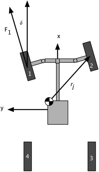
Figure 12.2 Planar automobile dynamical model.
The dynamical equations are written in the rotating frame. ![]() (12.5)
(12.5)
![]() (12.6)
(12.6)
![]() (12.7)
(12.7)
where the dynamic pressure is  (12.8)
and  (12.9)
The unit vector is  (12.10)
The normal force is mg, where g is the acceleration of gravity. The force at the tire contact point (where the tire touches the road) is20pt]Please provide the text citation for Fig. 12.3.

Figure 12.3 Wheel force and torque.
 (12.11)
where F
f
is the rolling friction and is ![]() (12.12)
(12.12)
where ![]() is the x-velocity in the tire frame. For front wheel drive cars the torque, T, is zero for the rear wheels. The contact friction is
is the x-velocity in the tire frame. For front wheel drive cars the torque, T, is zero for the rear wheels. The contact friction is  (12.13) The velocity term ensures that the friction force does not cause limit cycling.
The transformation from tire to body frame is  (12.14)
so that ![]() (12.15)
(12.15)
 (12.16)
The kinematic equations are ![]() (12.17)
(12.17)
and  (12.18)
12.3.3 Solution
The RHSAutomobile function is shown below.
function xDot = RHSAutomobile( ~, x, d )
% Constants
g = 9.806; % Acceleration of gravity (m/s^2)
n = length(x);
nS = 6; % Number of states
xDot = zeros(n,1);
nAuto = n/nS;
j = 1;
% State [j j+1 j+2 j+3 j+4 j+5]
% x y vX vY theta omega
for k = 1:nAuto
vX = x(j+2,1);
vY = x(j+3,1);
theta = x(j+4,1);
omega = x(j+5,1);
% Car angle
c = cos(theta);
s = sin(theta);
% Inertial frame
v = [c -s;s c]*[vX;vY];
delta = d.car(k).delta;
c = cos(delta);
s = sin(delta);
mCToT = [c s;-s c];
% Find the rolling resistance of the tires
vTire = mCToT*[vX;vY];
f0 = d.car(k).fRR(1);
K1 = d.car(k).fRR(2);
fRollingF = f0 + K1*vTire(1)^2;
fRollingR = f0 + K1*vX^2;
% This is the side force friction
fFriction = d.car(k).cF*d.car(k).mass*g;
fT = d.car(k).radiusTire*d.car(k).torque;
fF = [fT - fRollingF;-vTire(2)*fFriction];
fR = [ - fRollingR;-vY *fFriction];
% Tire forces
f1 = mCToT’*fF;
f2 = f1;
f3 = fR;
f4 = f3;
% Aerodynamic drag
vSq = vX^2 + vY^2;
vMag = sqrt(vSq);
q = 0.5*1.225*vSq;
fDrag = q*[d.car(k).cDF*d.car(k).areaF*vX;...
d.car(k).cDS*d.car(k).areaS*vY]/vMag;
% Force summations
f = f1 + f2 + f3 + f4 - fDrag;
% Torque
T = Cross2D( d.car(k).r(:,1), f1 ) + Cross2D( d.car(k).r(:,2), f2 ) + ...
Cross2D( d.car(k).r(:,3), f3 ) + Cross2D( d.car(k).r(:,4), f4 );
% Right hand side
xDot(j, 1) = v(1);
xDot(j+1,1) = v(2);
xDot(j+2,1) = f(1)/d.car(k).mass + omega*vY;
xDot(j+3,1) = f(2)/d.car(k).mass - omega*vX;
xDot(j+4,1) = omega;
xDot(j+5,1) = T/d.car(k).inr;
j = j + nS;
end
function c = Cross2D( a, b )
%% Cross2D
c = a(1)*b(2) - a(2)*b(1);
The Kalman filter’s right-hand side is just the differential equations ![]() (12.19)
(12.19)
![]() (12.20)
(12.20)
![]() (12.21)
(12.21)
![]() (12.22)
(12.22)
The dot means time derivative or rate of change with time. These are the state equations for the automobile. This model says that the position change with time is proportional to the velocity. It also says the velocity is constant. Information about velocity changes will come solely from the measurements. We also don’t model the angle or angular rate. This is because we aren’t getting information about it from the radar. However, you might try including it!
The RHSAutomobileXY function is shown below; it is only two lines of code!
function xDot = RHSAutomobileXY( ~, x, ~ )
xDot = [x(3:4);0;0];
12.4 Automobile Simulation and the Kalman Filter
12.4.1 Problem
You want to track a car using radar measurements to track an automobile maneuvering around your car. Cars may appear and disappear at any time. The radar measurement needs to be turned into the position and velocity of the tracked car. In between radar measurements you want to make your best estimate of where the automobile will be at a given time.
12.4.2 Solution
The solution is to implement a UKF to take radar measurements and update a dynamical model of the tracked automobile.
12.4.3 How It Works
The demonstration simulation is the same simulation used to demonstrate the multiple-hypothesis system tracking. This simulation just demonstrates the Kalman filter. Since the Kalman filter is the core of the package, it is important that it work well before adding the measurement assignment part.
MHTDistanceUKF finds the MHT distance for use in gating computations using the UKF. The measurement function is of the form h(x, d), where d is the UKF data structure. MHTDistanceUKF uses sigma points. The code is similar to UKFUpdate. As the uncertainty gets smaller, the residual must be smaller to remain within the gate.
function [k, del] = MHTDistanceUKF( d )
% Get the sigma points
pS = d.c*chol(d.p)’;
nS = length(d.m);
nSig = 2*nS + 1;
mM = repmat(d.m,1,nSig);
if( length(d.m) == 1 )
mM = mM’;
end
x = mM + [zeros(nS,1) pS -pS];
[y, r] = Measurement( x, d );
mu = y*d.wM;
b = y*d.w*y’ + r;
del = d.y - mu;
k = del’*(bdel);
function [y, r] = Measurement( x, d )
%% Measurement from the sigma points
nSigma = size(x,2);
lR = length(d.r);
y = zeros(lR,nSigma);
r = d.r;
iR = 1:lR;
for j = 1:nSigma
f = feval( d.hFun, x(:,j), d.hData );
y(iR,j) = f;
r(iR,iR) = d.r;
The simulation UKFAutomobileDemo uses a car data structure to contain all of the car information. A MATLAB function AutomobileInitialize takes parameter pairs and builds the data structure. This is a lot cleaner than assigning the individual fields in your script. It will return a default data structure if nothing is entered as an argument.
The first part of the demo, shown in the following listing, is the automobile simulation. It generates the measurements of the automobile positions to be used by the Kalman filter.
%% Initialize
% Set the seed for the random number generators.
% If the seed is not set each run will be different.
seed = 45198;
rng(seed);
% Car control
laneChange = 1;
% Clear the data structure
d = struct;
% Car 1 has the radar
d.car(1) = AutomobileInitialize( ...
’mass’, 1513,...
’position␣tires’, [1.17 1.17 -1.68 -1.68; -0.77 0.77 -0.77 0.77], ...
’frontal␣drag␣coefficient’, 0.25, ...
’side␣drag␣coefficient’, 0.5, ...
’tire␣friction␣coefficient’, 0.01, ...
’tire␣radius’, 0.4572, ...
’engine␣torque’, 0.4572*200, ...
’rotational␣inertia’, 2443.26, ...
’rolling␣resistance␣coefficients’, [0.013 6.5e-6], ...
’height␣automobile’, 2/0.77, ...
’side␣and␣frontal␣automobile␣dimensions’, [1.17+1.68 2*0.77]);
% Make the other car identical
d.car(2) = d.car(1);
nAuto = length(d.car);
% Velocity set points for the cars
vSet = [12 13];
% Time step setup
dT = 0.1;
tEnd = 20*60;
tLaneChange = 10*60;
tEndPassing = 6*60;
n = ceil(tEnd/dT);
% Car initial states
x = [140; 0;12;0;0;0;...
0; 0;11;0;0;0];
% Radar - the radar model has a field of view and maximum range
% Range drop off or S/N is not modeled
m = length(x)-1;
dRadar.kR = [ 7:6:m; 8:6:m]; % State position indices
dRadar.kV = [ 9:6:m;10:6:m]; % State velocity indices
dRadar.kT = 11:6:m; % State yaw angle indices
dRadar.noise = 0.1*[0.02;0.001;0.001]; % [range; range rate; azimuth]
dRadar.fOV = pi/4; % Field of view
dRadar.maxRange = inf;
dRadar.noLimits = 0; % Limits are checked (fov and range)
% Plotting
yP = zeros(3*(nAuto-1),n);
vP = zeros(nAuto-1,n);
xP = zeros(length(x)+2*nAuto,n);
s = 1:6*nAuto;
%% Simulate
t = (0:(n-1))*dT;
fprintf(1,’ Running␣the␣simulation...’);
for k = 1:n
% Plotting
xP(s,k) = x;
j = s(end)+1;
for i = 1:nAuto
p = 6*i-5;
d.car(i).x = x(p:p+5);
xP(j:j+1,k) = [d.car(i).delta;d.car(i).torque];
j = j + 2;
end
% Get radar measurements
dRadar.theta = d.car(1).x(5);
dRadar.t = t(k);
dRadar.xR = x(1:2);
dRadar.vR = x(3:4);
[yP(:,k), vP(:,k)] = AutoRadar( x, dRadar );
% Implement Control
% For all but the passing car control the velocity
d.car(1).torque = -10*(d.car(1).x(3) - vSet(1));
% The active car
if( t(k) < tEndPassing )
d.car(2) = AutomobilePassing( d.car(2), d.car(1), 3, 1.3, 10 );
elseif ( t(k) > tLaneChange && laneChange )
d.car(2) = AutomobileLaneChange( d.car(2), 10, 3, 12 );
else
d.car(2).torque = -10*(d.car(2).x(3) - vSet(2));
end
% Integrate
x = RungeKutta(@RHSAutomobile, 0, x, dT, d );
end
fprintf(1,’DONE. ’);
% The state of the radar host car
xRadar = xP(1:6,:);
% Plot the simulation results
NewFigure( ’Auto’ )
kX = 1:6:length(x);
kY = 2:6:length(x);
c = ’bgrcmyk’;
j = floor(linspace(1,n,20));
for k = 1:nAuto
plot(xP(kX(k),j),xP(kY(k),j),[c(k) ’.’]);
hold on
end
legend(’Auto␣1’,’Auto␣2’);
for k = 1:nAuto
plot(xP(kX(k),:),xP(kY(k),:),c(k));
end
xlabel(’x␣(m)’);
ylabel(’y␣(m)’);
set(gca,’ylim’,[-5 5]);
grid
The second part of the demo, shown in this listing, processes the measurements in the UKF to generate the estimates of the automobile track.
%% Implement UKF
% Covariances
r0 = diag(dRadar.noise.^2); % Measurement 1-sigma
q0 = [1e-7;1e-7;.1;.1]; % The baseline plant covariance diagonal
p0 = [5;0.4;1;0.01].^2; % Initial state covariance matrix diagonal
% Each step is one scan
ukf = KFInitialize( ’ukf’,’f’,@RHSAutomobileXY,’alpha’,1,...
’kappa’,0,’beta’,2,’dT’,dT,’fData’,struct(’f’,0),...
’p’,diag(p0),’q’,diag(q0),’x’,[0;0;0;0],’hData’,struct(’theta’,0),...
’hfun’,@AutoRadarUKF,’m’,[0;0;0;0],’r’,r0);
ukf = UKFWeight( ukf );
% Size arrays
k1 = find( vP > 0 );
k1 = k1(1);
% Limit to when the radar is tracking
n = n - k1 + 1;
yP = yP(:,k1:end);
xP = xP(:,k1:end);
pUKF = zeros(4,n);
xUKF = zeros(4,n);
dMHTU = zeros(1,n);
t = (0:(n-1))*dT;
for k = 1:n
% Prediction step
ukf.t = t(k);
ukf = UKFPredict( ukf );
% Update step
ukf.y = yP(:,k);
ukf = UKFUpdate( ukf );
% Compute the MHT distance
dMHTU(1,k) = MHTDistanceUKF( ukf );
% Store for plotting
pUKF(:,k) = diag(ukf.p);
xUKF(:,k) = ukf.m;
end
% Transform the velocities into the inertial frame
for k = 1:n
c = cos(xP(5,k));
s = sin(xP(5,k));
cCarToI = [c -s;s c];
xP(3:4,k) = cCarToI*xP(3:4,k);
c = cos(xP(11,k));
s = sin(xP(11,k));
cCarToI = [c -s;s c];
xP(9:10,k) = cCarToI*xP(9:10,k);
end
% Relative position
dX = xP(7:10,:) - xP(1:4,:);
%% Plotting
[t,tL] = TimeLabel(t);
% Plot just select states
k = [1:4 7:10];
yL = {’p_x’ ’p_y’ ’p_{v_x}’ ’p_{v_y}’};
pS = {[1 5] [2 6] [3 7] [4 8]};
PlotSet(t, pUKF, ’x␣label’, tL,’y␣label’, yL,’figure␣title’, ’Covariance’, ’plot␣title’, ’Covariance’);
PlotSet(t, [xUKF;dX], ’x␣label’, tL,’y␣label’,{’x’ ’y’ ’v_x’ ’v_y’},...
’plot␣title’,’UKF␣State:␣Blue␣is␣UKF,␣Green␣is␣Truth’,’figure␣title’,’UKF␣State’,’plot␣set’, pS );
PlotSet(t, dMHTU, ’x␣label’, tL,’y␣label’,’d␣(m)’, ’plot␣title’,’MHT␣Distance␣UKF’, ’figure␣title’,’MHT␣Distance␣UKF’,’plot␣type’,’ylog’);
The results of the script are shown in Figure 12.4, Figure 12.5, and Figure 12.6.

Figure 12.4 Automobile trajectories.

Figure 12.5 The true states and UKF estimated states.

Figure 12.6 The MHT distance between the automobiles during the simulation. Notice the spike in distance when the automobile maneuver starts.
12.5 Perform MHT on the Radar Data
12.5.1 Problem
You want to use hypothesis testing to track multiple cars. You need to take measurements returned by the radar and assign them methodically to the state histories, that is, position and velocity histories, of the automobiles. The radar doesn’t know one car from the other so you need a methodical and repeatable way to assign radar pings to tracks.
12.5.2 Solution
The solution is to implement track-oriented MHT. This system will learn the trajectories of all cars that are visible to the radar system.
Figure 12.7 shows the general tracking problem. Two scans of data are shown. When the first scan is done there are two tracks. The uncertainty ellipsoids are shown and they are based on all previous information. In the k − 1 scan three measurements are observed. 1 and 3 are within the ellipsoids of the two tracks but 2 is in both. It may be a measurement of either of the tracks or a spurious measurement. In scan k four measurements are taken. Only measurement 4 is in one of the uncertainty ellipsoids. 3 might be interpreted as spurious, but it is actually caused by a new track from a third vehicle that separates from the blue track. 1 is outside the red ellipsoid but is actually a good measurement of the red track and (if correctly interpreted) indicates that the model is erroneous. 4 is a good measurement of the blue track and indicates that the model is valid. The illustration shows how the tracking system should behave but without the tracks it would be difficult to interpret the measurements. A measurement can be valid, spurious, or a new track.

Figure 12.7 Tracking problem.
We define a contact as an observation where the signal-to-noise ratio is above a certain threshold. The observation then constitutes a measurement. Low signal-to-noise ratio observations can happen in both optical and radar systems. Thresholding reduces the number of observations that need to be associated with tracks but may lose valid data. An alternative is to treat all observations as contact but adjust the measurement error accordingly.
Valid measurements must then be assigned to tracks. An ideal tracking system would be able to categorize each measurement accurately and then assign them to the correct track. The system must also be able to identify new tracks and remove tracks that no longer exist.
If we were confident that we were only tracking one vehicle, all of the data might be incorporated into the state estimate. An alternative is to incorporate only the data within the covariance ellipsoids and treat the remainders as outliers. If the latter strategy were taken, it would be sensible to remember that data in case future measurements also were “outliers,” in which case the filter might go back and incorporate different sets of outliers into the solution. This could easily happen if the model were invalid, for example, if the vehicle, which had been coasting, suddenly began maneuvering and the filter model did not allow for maneuvers.
In classical multiple-target tracking [6], the problem is divided into two steps, association and estimation. Step 1 associates contacts with targets and step 2 estimates each target’s state. Complications arise when there is more than one reasonable way to associate contacts with targets. The MHT approach is to form alternative hypotheses to explain the source of the observations. Each hypothesis assigns observations to targets or false alarms.
There are two approaches to MHT [3]. The first, following Reid [5], operates within a structure in which hypotheses are continually maintained and updated as observation data are received. In the second, the track-oriented approach to MHT, tracks are initiated, updated, and scored before being formed into hypotheses. The scoring process consists of comparing the likelihood that the track represents a true target versus the likelihood that it is a collation of false alarms. Thus, unlikely tracks can be deleted before the next stage in which tracks are formed into hypotheses.
The track-oriented approach recomputes the hypotheses using the newly updated tracks after each scan of data is received. Rather than maintaining, and expanding, hypotheses from scan to scan, the track-oriented approach discards the hypotheses formed on scan k − 1. The tracks that survive pruning are predicted to the next scan k where new tracks are formed, using the new observations, and reformed into hypotheses. Except for the necessity to delete some tracks based upon low probability or N-scan pruning, no information is lost because the track scores, which are maintained, contain all the relevant statistical data. MHT terms are defined in Table 12.1.
Table 12.1 MHT Terms
Term | Definition |
Clutter | Transient objects of no interest to the tracking system |
Cluster | A collection of tracks that are linked by common observations |
Family | A set of tracks with a common root node. At most one track per family can be included in a hypothesis. A family can represent at most one target |
Hypothesis | A set of tracks that do not share any common observations |
N-Scan Pruning | Using the track scores from the last N scans of data to prune tracks. The count starts from a root node. When the tracks are pruned, a new root node is established |
Observation | A measurement that indicates the presence of an object. The observation may be of a target or be spurious |
Pruning | Removal of low-score tracks |
Root Node | An established track to which observations can be attached and which may spawn additional tracks |
Scan | A set of data taken simultaneously |
Target | An object being tracked |
Trajectory | The path of a target |
Track | A trajectory that is propagated |
Track Branch | A track in a family that represents a different data association hypothesis. Only one branch can be correct |
Track Score | The log-likelihood ratio for a track |
Track scoring is done using log-likelihood ratios: ![$$displaystyle{ L(K) =log [mathrm{LR}(K)] =sum _{ k=1}^{K}left [mathrm{LLR}_{ K}(k) +mathrm{ LLR}_{S}(k)
ight ] +log [L_{0}] }$$](http://images-20200215.ebookreading.net/5/1/1/9781484222508/9781484222508__matlab-machine-learning__9781484222508__A420697_1_En_12_Chapter_Equ23.gif) (12.23)
(12.23)
where the subscript K denotes kinematic and the subscript S denotes signal. It is assumed that the two are statistically independent.  (12.24)
where H
1 and H
0 are the true target and false alarm hypotheses. log is the natural logarithm. The likelihood ratio for the kinematic data is the probability that the data are a result of the true target divided by the probability that the data are from a false alarm:
 (12.25)
where M is the measurement dimension, V
C
is the measurement volume, S = HPT
T
+ R is the measurement residual covariance matrix, and d
2 = y
T
S
−1
y is the normalized statistical distance for the measurement defined by the residual y and the covariance matrix S. The numerator is the multivariate Gaussian.
The following are the rules for each measurement:
Each measurement creates a new track.
Each measurement in each gate updates the existing track. If there is more than one measurement in a gate, the existing track is duplicated with the new measurement.
All existing tracks are updated with a “missed” measurement, creating a new track.
Figure 12.8 gives an example. There are two tracks and three measurements. All three measurements are in the gate for track 1, but only one is in the gate for track 2. Each measurement produces a new track. The three measurements produce three tracks based on track 1 and the one measurement produces one track based on track 2. Each track also spawns a new track assuming that there was no measurement for the track. Thus, in this case three measurements and two tracks result in nine tracks. Tracks 7–9 are initiated based only on the measurement, which may not be enough information to initiate the full state vector. If this is the case, there would be an infinite number of tracks associated with each measurement, not just one new track. If we have a radar measurement we have azimuth, elevation, range, and range rate. This gives all position states and one velocity state.

Figure 12.8 Measurement and gates. M0 is an “absent” measurement.
12.5.3 How It Works
Track management is done by MHTTrackMgmt. This implements track-oriented MHT. It creates new tracks each scan. A new track is created
For each measurement
For any track which has more than one measurement in its gate
For each existing track with a ”null” measurement
Tracks are pruned to eliminate those of low probability and find the hypothesis which includes consistent tracks. Consistent tracks do not share any measurements.
This is typically used in a loop in which each step has new measurements, known as “scans.” Scan is radar terminology for a rotating antenna beam. A scan is a set of sensor data taken at the same time.
The simulation can go in a loop to generate y or you can run the simulation separately and store the measurements in y. This can be helpful when you are debugging your MHT code.
For real-time systems y would be read in from your sensors. The MHT code would update every time you received new measurements. The code snippet below is from the header of MHTTrackMgmt, showing the overall approach to implementation.
zScan = [];
for k = 1:n
zScan = AddScan( y(:,k), [], [], [], zScan ) ;
[b, trk, sol, hyp] = MHTTrackMgmt( b, trk, zScan, trkData, k, t );
MHTGUI(trk,sol);
for j = 1:length(trk)
trkData.fScanToTrackData.v = myData
end
if( ~isempty(zScan) && makePlots )
TOMHTTreeAnimation( ’update’, trk );
end
t = t + dT;
end
Reference [1] provides good background reading, but the code in this function is not based on the reference. Other good references are books and papers by Blackman including [2] and [4].
%% MHTTrackMgmt - manages tracks
%
%% Form:
% [b, trk, sol, hyp] = MHTTrackMgmt( b, trk, zScan, d, scan, t )
%
%% Description
% Manage Track Oriented Multiple Hypothesis Testing tracks.
%
% Performs track reduction and track pruning.
%
% It creates new tracks each scan. A new track is created
% - for each measurement
% - for any track which has more than one measurement in its gate
% - for each existing track with a "null" measurement.
%
% Tracks are pruned to eliminate those of low probability and find the
% hypothesis which includes consistent tracks. Consistent tracks do
% not share any measurements.
%
% This is typically used in a loop in which each step has new
% measurements, known as "scans". Scan is radar terminology for a
% rotating antenna beam. A scan is a set of sensor data taken at the
% ame time.
%
% The simulation can go in ths loop to generate y or you can run the
% simulation separately and store the measurements in y. This can be
% helpful when you are debugging your MHT code.
%
% For real time systems y would be read in from your sensors. The MHT
% code would update every time you received new measurements.
%
% zScan = [];
%
% for k = 1:n
%
% zScan = AddScan( y(:,k), [], [], [], zScan ) ;
%
% [b, trk, sol, hyp] = MHTTrackMgmt( b, trk, zScan, trkData, k, t );
%
% MHTGUI(trk,sol);
%
% for j = 1:length(trk)
% trkData.fScanToTrackData.v = myData
% end
%
% if( ~isempty(zScan) && makePlots )
% TOMHTTreeAnimation( ’update’, trk );
% end
%
% t = t + dT;
%
% end
%
% The reference provides good background reading but the code in this
% function is not based on the reference. Other good references are
% books and papers by Blackman.
%
%% Inputs
% b (m,n) [scans, tracks]
% trk (:) Track data structure
% zScan (1,:) Scan data structure
% d (1,1) Track management parameters
% scan (1,1) The scan id
% t (1,1) Time
%
%% Outputs
% b (m,1) [scans, tracks]
% trk (:) Track data structure
% sol (.) Solution data structure from TOMHTAssignment
% hyp (:) Hypotheses
%
%% Reference
% A. Amditis1, G. Thomaidis1, P. Maroudis, P. Lytrivis1 and
% G. Karaseitanidis1, "Multiple Hypothesis Tracking
% Implementation ," www.intechopen.com.
function [b, trk, sol, hyp] = MHTTrackMgmt( b, trk, zScan, d, scan, t )
% Warn the user that this function does not have a demo
if( nargin < 1 )
disp(’Error:␣6␣inputs␣are␣required’);
return;
end
MLog(’add’,sprintf(’=============␣SCAN␣%d␣==============’,scan),scan);
% Add time to the filter data structure
for j = 1:length(trk)
trk(j).filter.t = t;
end
% Remove tracks with an old scan history
earliestScanToKeep = scan-d.nScan;
keep = zeros(1,length(trk));
for j=1:length(trk);
if( isempty(trk(j).scanHist) || max(trk(j).scanHist)>=earliestScanToKeep )
keep(j) = 1;
end
end
if any(~keep)
txt = sprintf(’DELETING␣%d␣tracks␣with␣old␣scan␣histories. ’, length(find (~keep)));
MLog(’add’,txt,scan);
end
trk = trk( find(keep) );
nTrk = length(trk);
% Remove old scanHist and measHist entries
for j=1:nTrk
k = find(trk(j).scanHist<earliestScanToKeep);
if( ~isempty(k) )
trk(j).measHist(k) = [];
trk(j).scanHist(k) = [];
end
end
% Above removal of old entries could result in duplicate tracks
%--------------------------------------------------------------
dup = CheckForDuplicateTracks( trk, d.removeDuplicateTracksAcrossAllTrees );
trk = RemoveDuplicateTracks( trk, dup, scan );
nTrk = length(trk);
% Perform the Kalman Filter prediction step
%------------------------------------------
for j = 1:nTrk
trk(j).filter = feval( d.predict, trk(j).filter );
trk(j).mP = trk(j).filter.m;
trk(j).pP = trk(j).filter.p;
trk(j).m = trk(j).filter.m;
trk(j).p = trk(j).filter.p;
end
% Track assignment
% 1. Each measurement creates a new track
% 2. One new track is created by adding a null measurement to each existing
% track
% 3. Each measurement within a track’s gate is added to a track. If there
% are more than 1 measurement for a track create a new track.
%
% Assign to a track. If one measurement is within the gate we just assign
% it. If more than one we need to create a new track
nNew = 0;
newTrack = [];
newScan = [];
newMeas = [];
nS = length(zScan);
maxID = 0;
maxTag = 0;
for j = 1:nTrk
trk(j).d = zeros(1,nS);
trk(j).new = [];
for i = 1:nS
trk(j).filter.x = trk(j).m;
trk(j).filter.y = zScan(i);
trk(j).d(i) = feval( d.fDistance, trk(j).filter );
end
trk(j).gate = trk(j).d < d.gate;
hits = find(trk(j).gate==1);
trk(j).meas = [];
lHits = length(hits);
if( lHits > 0 )
if( lHits > 1)
for k = 1:lHits-1
newTrack(end+1) = j;
newScan(end+1) = trk(j).gate(hits(k+1));
newMeas(end+1) = hits(k+1);
end
nNew = nNew + lHits - 1;
end
trk(j).meas = hits(1);
trk(j).measHist(end+1) = hits(1);
trk(j).scanHist(end+1) = scan;
if( trk(j).scan0 == 0 )
trk(j).scan0 = scan;
end
end
maxID = max(maxID,trk(j).treeID);
maxTag = max(maxTag,trk(j).tag);
end
nextID = maxID+1;
nextTag = maxTag+1;
% Create new tracks assuming that existing tracks had no measurements
%--------------------------------------------------------------------
nTrk0 = nTrk;
for j = 1:nTrk0
if( ~isempty(trk(j).scanHist) && trk(j).scanHist(end) == scan )
% Add a copy of track "j" to the end with NULL measurement
%---------------------------------------------------------
nTrk = nTrk + 1;
trk(nTrk) = trk(j);
trk(nTrk).meas = [];
trk(nTrk).treeID = trk(nTrk).treeID; % Use the SAME track tree ID
trk(nTrk).scan0 = scan;
trk(nTrk).tag = nextTag;
nextTag = nextTag + 1; % increment next tag number
% The track we copied already had a measurement appended for this
% scan, so replace these entries in the history
%----------------------------------------------
trk(nTrk).measHist(end) = 0;
trk(nTrk).scanHist(end) = scan;
end
end
% Do this to notify us if any duplicate tracks are created
%---------------------------------------------------------
dup = CheckForDuplicateTracks( trk );
trk = RemoveDuplicateTracks( trk, dup, scan );
% Add new tracks for existing tracks which had multiple measurements
%-------------------------------------------------------------------
if( nNew > 0 )
nTrk = length(trk);
for k = 1:nNew
j = k + nTrk;
trk(j) = trk(newTrack(k));
trk(j).meas = newMeas(k);
trk(j).treeID = trk(j).treeID;
trk(j).measHist(end) = newMeas(k);
trk(j).scanHist(end) = scan;
trk(j).scan0 = scan;
trk(j).tag = nextTag;
nextTag = nextTag + 1;
end
end
% Do this to notify us if any duplicate tracks are created
dup = CheckForDuplicateTracks( trk );
trk = RemoveDuplicateTracks( trk, dup, scan );
nTrk = length(trk);
% Create a new track for every measurement
for k = 1:nS
nTrk = nTrk + 1;
% Use next track ID
%------------------
trkF = feval(d.fScanToTrack, zScan(i), d.fScanToTrackData, scan, nextID, nextTag );
if( isempty(trk) )
trk = trkF;
else
trk(nTrk) = trkF;
end
trk(nTrk).meas = k;
trk(nTrk).measHist = k;
trk(nTrk).scanHist= scan;
nextID = nextID + 1; % increment next track-tree ID
nextTag = nextTag + 1; % increment next tag number
end
% Exit now if there are no tracks
if( nTrk == 0 )
b = [];
hyp = [];
sol = [];
return;
end
% Do this to notify us if any duplicate tracks are created
dup = CheckForDuplicateTracks( trk );
trk = RemoveDuplicateTracks( trk, dup, scan );
nTrk = length(trk);
% Remove any tracks that have all NULL measurements
kDel = [];
if( nTrk > 1 ) % do this to prevent deletion of very first track
for j=1:nTrk
if( ~isempty(trk(j).measHist) && all(trk(j).measHist==0) )
kDel = [kDel j];
end
end
if( ~isempty(kDel) )
keep = setdiff(1:nTrk,kDel);
trk = trk( keep );
end
nTrk = length(trk);
end
% Compute track scores for each measurement
for j = 1:nTrk
if( ~isempty(trk(j).meas ) )
i = trk(j).meas;
trk(j).score(scan) = MHTTrackScore( zScan(i), trk(j).filter, d.pD, d.pFA, d.pH1, d.pH0 );
else
trk(j).score(scan) = MHTTrackScore( [], trk(j).filter, d.pD, d.pFA, d.pH1, d.pH0 );
end
end
% Find the total score for each track
nTrk = length(trk);
for j = 1:nTrk
if( ~isempty(trk(j).scanHist) )
k1 = trk(j).scanHist(1);
k2 = length(trk(j).score);
kk = k1:k2;
if( k1<length(trk(j).score)-d.nScan )
error(’The␣scanHist␣array␣spans␣back␣too␣far.’)
end
else
kk = 1;
end
trk(j).scoreTotal = MHTLLRUpdate( trk(j).score(kk) );
% Add a weighted value of the average track score
if( trk(j).scan0 > 0 )
kk2 = trk(j).scan0 : length(trk(j).score);
avgScore = min(0,MHTLLRUpdate( trk(j).score(kk2) ) / length(kk2));
trk(j).scoreTotal = trk(j).scoreTotal + d.avgScoreHistoryWeight * avgScore;
end
end
% Update the Kalman Filters
for j = 1:nTrk
if( ~isempty(zScan) && ~isempty(trk(j).meas) )
trk(j).filter.y = zScan(trk(j).meas);
trk(j).filter = feval( d.update, trk(j).filter );
trk(j).m = trk(j).filter.m;
trk(j).p = trk(j).filter.p;
trk(j).mHist(:,end+1) = trk(j).filter.m;
end
end
% Examine the tracks for consistency
duplicateScans = zeros(1,nTrk);
for j=1:nTrk
if( length(unique(trk(j).scanHist)) < length(trk(j).scanHist))
duplicateScans(j)=1;
end
end
% Update the b matrix and delete the oldest scan if necessary
b = MHTTrkToB( trk );
rr = rand(size(b,2),1);
br = b*rr;
if( length(unique(br))<length(br) )
MLog(’add’,sprintf(’DUPLICATE␣TRACKS!!! ’),scan);
end
% Solve for "M best" hypotheses
sol = TOMHTAssignment( trk, d.mBest );
% prune by keeping only those tracks whose treeID is present in the list of
% "M best" hypotheses
trk0 = trk;
if( d.pruneTracks )
[trk,kept,pruned] = TOMHTPruneTracks( trk, sol, d.hypScanLast );
b = MHTTrkToB( trk );
% Do this to notify us if any duplicate tracks are created
dup = CheckForDuplicateTracks( trk );
trk = RemoveDuplicateTracks( trk, dup, scan );
% Make solution data compatible with pruned tracks
if( ~isempty(pruned) )
for j=1:length(sol.hypothesis)
for k = 1:length(sol.hypothesis(j).trackIndex)
sol.hypothesis(j).trackIndex(k) = find( sol.hypothesis(j).trackIndex(k) == kept );
end
end
end
end
if( length(trk)<length(trk0) )
txt = sprintf(’Pruning:␣Reduce␣from␣%d␣to␣%d␣tracks. ’, length (trk0), length (trk));
MLog(’add’,txt,scan);
else
MLog(’add’,sprintf(’Pruning:␣All␣tracks␣survived. ’),scan);
end
% Form hypotheses
if( scan >= d.hypScanLast + d.hypScanWindow )
hyp = sol.hypothesis(1);
else
hyp = [];
end
function trk = RemoveDuplicateTracks( trk, dup, scan )
%% Remove duplicate tracks
if( ~isempty(dup) )
MLog(’update’,sprintf(’DUPLICATE␣TRACKS:␣%s ’,mat2str(dup)),scan);
kDup = unique(dup(:,2));
kUnq = setdiff(1:length(trk),kDup);
trk(kDup) = [];
dup2 = CheckForDuplicateTracks( trk );
if( isempty(dup2) )
txt = sprintf(’Removed␣%d␣duplicates,␣kept␣tracks:␣%s ’, length (kDup),mat2str(kUnq));
MLog(’add’,txt,scan);
else
error(’Still␣have␣duplicates.␣Something␣is␣wrong␣with␣this␣pruning.’)
end
end
MHTTrackMgmt uses hypothesis forming and track pruning from the following two recipes.
12.5.4 Hypothesis Formation
12.5.4.1 Problem
Form hypotheses about tracks.
12.5.4.2 Solution
Formulate as a mixed integer-linear programming (MILP) and solve using GNU Linear Programming Kit (GLPK).
12.5.4.3 How It Works
Hypotheses are sets of tracks with consistent data, that is, where no measurements are assigned to more than one track. The track-oriented approach recomputes the hypotheses using the newly updated tracks after each scan of data is received. Rather than maintaining, and expanding, hypotheses from scan to scan, the track-oriented approach discards the hypotheses formed on scan k − 1. The tracks that survive pruning are propagated to the next scan k where new tracks are formed, using the new observations, and reformed into hypotheses. Except for the necessity to delete some tracks based upon low probability, no information is lost because the track scores, which are maintained, contain all the relevant statistical data.
In MHT, a valid hypothesis is any compatible set of tracks. In order for two or more tracks to be compatible, they cannot describe the same object, and they cannot share the same measurement at any of the scans. The task in hypothesis formation is to find one or more combinations of tracks that (1) are compatible and (2) maximize some performance function.
Before discussing the method of hypothesis formation, it is useful to first consider track formation and how tracks are associated with unique objects. New tracks may be formed in one of two ways:
The new track is based on some existing track, with the addition of a new measurement.
The new track is NOT based on any existing tracks; it is based solely on a single new measurement.
Recall that each track is formed as a sequence of measurements across multiple scans. In addition to the raw measurement history, every track also contains a history of state and covariance data that is computed from a Kalman filter. When a new measurement is appended to an existing track, we are spawning a new track that includes all of the original track’s measurements, plus this new measurement. Therefore, the new track is describing the same object as the original track.
A new measurement can also be used to generate a completely new track that is independent of past measurements. When this is done, we are effectively saying that the measurement does not describe any of the objects that are already being tracked. It therefore must correspond to a new or different object.
In this way, each track is given an object ID to distinguish which object it describes. Within the context of track-tree diagrams, all of the tracks inside the same track-tree have the same object ID. For example, if at some point there are 10 separate track-trees, this means that 10 separate objects are being tracked in the MHT system. When a valid hypothesis is formed, it may turn out that only a few of these objects have compatible tracks.
The hypothesis formation step is formulated as an MILP and solved using GLPK. Each track is given an aggregate score that reflects the component scores attained from each measurement. The MILP formulation is constructed to select a set of tracks that add to give the highest score, such that
No two tracks have the same object ID.
No two tracks have the same measurement index for any scan.
In addition, we extended the formulation with an option to solve for multiple hypotheses, rather than just one. The algorithm will return the “M best” hypotheses, in descending order of score. This enables tracks to be preserved from alternate hypotheses that may be very close in score to the best.
The following code shows how hypothesis formation is done. GLPK is available for free. Its website includes installation instructions.
TOMHTAssignment generates hypotheses. The “b” matrix represents a stacked set of track-trees. Each row is a different path through a track-tree. Each column is a different scan. Values in the matrix are the index of the measurement for that scan. A valid hypothesis is a combination of rows of b (a combination of track-tree paths), such that the same measurement is not repeated. The solution vector “x” is an array with 0s and 1s that selects a set of track-tree paths. The objective is to find the hypothesis that maximizes the total score.
%% TOMHTASSIGNMENT - generates hypotheses
%
%% Form:
% d = TOMHTAssignment( trk, M, glpkParams );
%
%% Description
% Track oriented MHT assignment. Generates hypotheses.
%
% The "b" matrix represents a stacked set of track-trees.
% Each row is a different path through a track-tree
% Each column is a different scan
% Values in matrix are index of measurement for that scan
%
% A valid hypothesis is a combination of rows of b (a combination of
% track-tree paths), such that the same measurement is not repeated.
%
% Solution vector "x" is 0|1 array that selects a set of track-tree-paths.
%
% Objective is to find the hypothesis that maximizes total score.
%
%
%% Inputs
% trk (.) Data structure array of track information
% From this data we will obtain:
% b (nT,nS) Matrix of measurement IDs across scans
% trackScores (1,nT) Array of total track scores
% treeIDs (1,nT) Array of track ID numbers. A common ID across
% multiple tracks means they are in the same
% track-tree.
% M (1,1) Number of hypotheses to generate.
% glpkParams (.) Data structure with glpk parameters.
%
%% Outputs
% d (.) Data structure with fields:
% .nT Number of tracks
% .nS Number of scans
% .M Number of hypotheses
% .pairs Pairs of hypotheses for score constraints
% .nPairs Number of pairs
% .A Constraint matrix for optimization
% .b Constraint vector for optimization
% .c Cost vector for optimization
% .lb lower bounds on solution vector
% .ub upper bounds on solution vector
% .conType Constraint type array
% .varType Variable type array
% .x Solution vector for optimization
% .hypothesis(:) Array of hypothesis data
%
% d.hypothesis(:) Data strcuture array with fields:
% .treeID Vector of track-tree IDs in hypothesis
% .trackIndex Vector of track indices in hypothesis.
% Maps to rows of "b" matrix.
% .tracks Set of tracks in hypothesis. These are
% the selected rows of "b" matrix.
% .trackScores Vector of scores for selected tracks.
% .score Total score for hypothesis.
%
%% References
% Blackman, S. and R. Popoli, "Design and Analysis of Modern
% Tracking Systems," Artech House, 1999.
%% Copyright
% Copyright (c) 2012-2013 Princeton Satellite Systems, Inc.
% All rights reserved.
function d = TOMHTAssignment( trk, M, glpkParams )
%==================================
% --- OPTIONS ---
%
% Prevent tracks with all zeros
% from being selected?
%
preventAllZeroTracks = 0;
%
%
%
% Choose a scoring method:
% log-LR sum of log of likelihood ratios
% LR sum of likelihood ratios
% prob sum of probabilities
%
scoringMethod = ’log-LR’;
%
%==================================
% how many solutions to generate?
if( nargin<2 )
M = 2;
end
% GLPK parameters
if( nargin<5 )
% Searching time limit, in seconds.
% If this value is positive, it is decreased each
% time when one simplex iteration has been performed by the
% amount of time spent for the iteration, and reaching zero
% value signals the solver to stop the search. Negative
% value means no time limit.
glpkParams.tmlim = 10;
% Level of messages output by solver routines:
% 0 - No output.
% 1 - Error messages only.
% 2 - Normal output.
% 3 - Full output (includes informational messages).
glpkParams.msglev = 0;
end
% extract "b" matrix
b = MHTTrkToB(trk);
% the track tree IDs
treeIDs = [trk.treeID];
scans = unique([trk.scanHist]);
scan = max(scans);
% the track scores
switch lower(scoringMethod)
case ’log-lr’
% the "scoreTotal" field is the sum of log likelihood ratios
trackScores = [trk.scoreTotal];
case ’lr’
% Redefine scores this way rather than sum of log of each scan score
trackScores = zeros(1,nT);
for j=1:nT
if( ~isempty(trk(j).scanHist) )
trackScores(j) = sum(trk(j).score(trk(j).scanHist(1):end));
else
trackScores(j) = sum(trk(j).score);
end
end
case ’prob’
error(’Probability␣scoring␣not␣implemented␣yet.’)
end
% remove occurrence of "inf"
kinf = find(isinf(trackScores));
trackScores(kinf) = sign(trackScores(kinf))*1e8;
% remove treeIDs column from b
b = b(:,2:end);
[nT,nS] = size(b);
nCon = 0; % number of constraints not known yet. compute below
nVar = nT; % number of variables is equal to total # track-tree-paths
% compute number of constraints
for i=1:nS
% number of measurements taken for this scan
nMeasForThisScan = max(b(:,i));
nCon = nCon + nMeasForThisScan;
end
% Initialize A, b, c
d.A = zeros(nCon,nVar*M);
d.b = zeros(nCon,1);
d.c = zeros(nVar*M,1);
d.conType = char(zeros(1,nCon));
d.varType = char(zeros(1,nVar));
for i=1:M
col0 = (i-1)*nT;
for j=1:nT
d.varType(col0+j) = ’B’; % all binary variables
%d.c(col0+j) = trackProb(j);
d.c(col0+j) = trackScores(j);
%d.c(col0+j) = trackScoresPos(j);
end
end
% coefficients for unique tag generation
%coeff = 2.^[0 : 1 : nT-1];
conIndex = 0;
col0 = 0;
% find set of tracks that have all zeros, if any
bSumCols = sum(b,2);
kAllZeroTracks = find(bSumCols==0);
for mm = 1:M
% for each track-tree ID
treeIDsU = unique(treeIDs);
for i=1:length(treeIDsU)
rows = find(treeIDs==treeIDsU(i));
% for each row of b with this track ID
conIndex = conIndex+1;
for j=rows
d.A(conIndex,col0+j) = 1;
d.b(conIndex) = 1;
d.conType(conIndex) = ’U’; % upper bound: A(conIndex ,:)*x <= 1
end
end
% for each scan
for i=1:nS
% number of measurements taken for this scan
nMeasForThisScan = max(b(:,i));
% for each measurement (not 0)
for k=1:nMeasForThisScan
% get rows of b matrix with this measurement index
bRowsWithMeasK = find(b(:,i)==k);
conIndex = conIndex+1;
% for each row
for j = bRowsWithMeasK
d.A(conIndex,col0+j) = 1;
d.b(conIndex) = 1;
d.conType(conIndex) = ’U’; % upper bound: A(conIndex ,:)*x <= 1
end
end
end
% prevent tracks with all zero measurements from being selected
if( preventAllZeroTracks )
for col = kAllZeroTracks
conIndex = conIndex+1;
d.A(conIndex,col) = 1;
d.b(conIndex) = 0;
d.conType(conIndex) = ’S’;
end
end
col0 = col0 + nT;
end
% variable bounds
d.lb = zeros(size(d.c));
d.ub = ones(size(d.c));
% add set of constraints / vars for each pair of solutions
if( M>1 )
pairs = nchoosek(1:M,2);
nPairs = size(pairs,1);
for i=1:nPairs
k1 = pairs(i,1);
k2 = pairs(i,2);
xCol1 = (k1-1)*nT+1 : k1*nT;
xCol2 = (k2-1)*nT+1 : k2*nT;
% enforce second score to be less than first score
% c1*x1 - c2*x2 >= tol
conIndex = conIndex + 1;
d.A(conIndex,xCol1) = d.c(xCol1);
d.A(conIndex,xCol2) = -d.c(xCol2);
d.b(conIndex) = 10; % must be non-negative and small
d.conType(conIndex) = ’L’;
end
else
pairs = [];
nPairs = 0;
end
if( nT>1 )
% call glpk to solve for optimal hypotheses
%glpkParams.msglev = 3; % use this for detailed GLPK printout
d.A( abs(d.A)<eps ) = 0;
d.b( abs(d.b)<eps ) = 0;
[d.x,~,status] = glpk(d.c,d.A,d.b,d.lb,d.ub,d.conType,d.varType,-1,glpkParams);
switch status
case 1
MLog(’add’,sprintf(’GLPK:␣1:␣solution␣is␣undefined. ’),scan);
case 2
MLog(’add’,sprintf(’GLPK:␣2:␣solution␣is␣feasible. ’),scan);
case 3
MLog(’add’,sprintf(’GLPK:␣3:␣solution␣is␣infeasible. ’),scan);
case 4
MLog(’add’,sprintf(’GLPK:␣4:␣no␣feasible␣solution␣exists. ’),scan);
case 5
MLog(’add’,sprintf(’GLPK:␣5:␣solution␣is␣optimal. ’),scan);
case 6
MLog(’add’,sprintf(’GLPK:␣6:␣solution␣is␣unbounded. ’),scan);
otherwise
MLog(’add’,sprintf(’GLPK:␣%d ’,status),scan);
end
else
d.x = ones(M,1);
end
d.nT = nT;
d.nS = nS;
d.M = M;
d.pairs = pairs;
d.nPairs = nPairs;
d.trackMat = b;
for mm=1:M
rows = (mm-1)*nT+1 : mm*nT;
sel = find(d.x(rows));
d.hypothesis(mm).treeID = treeIDs(sel);
d.hypothesis(mm).tracks = b(sel,:);
for j=1:length(sel)
d.hypothesis(mm).meas{j} = trk(sel).measHist;
d.hypothesis(mm).scans{j} = trk(sel).scanHist;
end
d.hypothesis(mm).trackIndex = sel;
d.hypothesis(mm).trackScores = trackScores(sel);
d.hypothesis(mm).score = sum(trackScores(sel));
end
12.5.5 Track Pruning
12.5.5.1 Problem
We need to prune tracks to prevent an explosion of tracks.
12.5.5.2 Solution
Implement N-scan track pruning.
12.5.5.3 How It Works
The N-scan track pruning is carried out at every step using the last n scans of data. We use a pruning method in which the following tracks are preserved:
Tracks with the “N” highest scores
Tracks that are included in the “M best” hypotheses
Tracks that have both (1) the object ID and (2) the first “P” measurements found in the “M best” hypotheses
We use the results of hypothesis formation to guide track pruning. The parameters N, M, P can be tuned to improve performance. The objective with pruning is to reduce the number of tracks as much as possible while not removing any tracks that should be part of the actual true hypothesis.
The second item listed above is to preserve all tracks included in the “M best” hypotheses. Each of these is a full path through a track-tree, which is clear. The third item listed above is similar, but less constrained. Consider one of the tracks in the “M best” hypotheses. We will preserve this full track. In addition, we will preserve all tracks that stem from scan “P” of this track.
Figure 12.9 provides an example of which tracks in a track-tree might be preserved. The diagram shows 17 different tracks over 5 scans. The green track represents one of the tracks found in the set of “M best” hypotheses, from the hypothesis formation step. This track would be preserved. The orange tracks all stem from the node in this track at scan 2. These would be preserved if we set P = 2 from the description above. The following code shows how track pruning is done.

Figure 12.9 Track pruning example
function [tracksP,keep,prune,d] = TOMHTPruneTracks( tracks, soln, scan0, opts )
% default value for starting scan index
if( nargin<3 )
scan0 = 0;
end
% default algorithm options
if( nargin<4 )
opts.nHighScoresToKeep = 5;
opts.nFirstMeasMatch = 3;
end
% increment the # scans to match
opts.nFirstMeasMatch = opts.nFirstMeasMatch + scan0;
% output structure to record which criteria resulted in preservation of
% which tracks
d.bestTrackScores = [];
d.bestHypFullTracks = [];
d.bestHypPartialTracks = [];
% number of hypotheses, tracks, scans
nHyp = length(soln.hypothesis);
nTracks = length(tracks);
nScans = size(soln.hypothesis(1).tracks,2);
% must limit # required matching measurements to # scans
if( opts.nFirstMeasMatch > nScans )
opts.nFirstMeasMatch = nScans;
end
% if # high scores to keep equals or exceeds # tracks
% then just return original tracks
if( opts.nHighScoresToKeep > nTracks )
tracksP = tracks;
keep = 1:length(tracks);
prune = [];
d.bestTrackScores = keep;
return
end
% get needed vectors out of trk array
scores = [tracks.scoreTotal];
treeIDs = [tracks.treeID];
% get list of all treeIDs in hypotheses
treeIDsInHyp = [];
for j=1:nHyp
treeIDsInHyp = [treeIDsInHyp, soln.hypothesis(j).treeID];
end
treeIDsInHyp = unique(treeIDsInHyp);
% create a matrix of hypothesis data with ID and tracks
hypMat = [soln.hypothesis(1).treeID’, soln.hypothesis(1).tracks];
for j=2:nHyp
for k=1:length(soln.hypothesis(j).treeID)
% if this track ID is not already included,
if( all(soln.hypothesis(j).treeID(k) ~= hypMat(:,1)) )
% then append this row to bottom of matrix
hypMat = [hypMat; ...
soln.hypothesis(j).treeID(k), soln.hypothesis(j).tracks(k,:)];
end
end
end
% Initialize "keep" array to all zeros
keep = zeros(1,nTracks);
% Keep tracks with the "N" highest scores
if( opts.nHighScoresToKeep>0 )
[~,ks] = sort(scores,2,’descend’);
index = ks(1:opts.nHighScoresToKeep);
keep( index ) = 1;
d.bestTrackScores = index(:)’;
end
% Keep tracks in the "M best" hypotheses
for j=1:nHyp
index = soln.hypothesis(j).trackIndex;
keep( index ) = 1;
d.bestHypFullTracks = index(:)’;
end
% If we do not require any measurements to match,
% then include ALL tracks with an ID contained in "M best hypotheses"
if( opts.nFirstMeasMatch == 0 )
% This means we include the entire track-tree for those IDs in included
% in the set of best hypotheses.
for k = 1:length(trackIDsInHyp)
index = find(treeIDs == trackIDsInHyp(k));
keep( index ) = 1;
d.bestHypPartialTracks = index(:)’;
end
% If the # measurements we require to match is equal to # scans, then
% this is equivalent to the set of tracks in the hypothesis solution.
elseif( opts.nFirstMeasMatch == nScans )
% We have already included these tracks, so nothing more to do here.
else
% Otherwise, we have some subset of measurements to match.
% Find the set of tracks that have:
% 1. track ID and
% 2. first "P" measurements
% included in "M best" hypotheses
nTracksInHypSet = size(hypMat,1);
tagMap = rand(opts.nFirstMeasMatch+1,1);
b = MHTTrkToB2( tracks );
trkMat = [ trackIDs’, b ];
trkTag = trkMat(:,1:opts.nFirstMeasMatch+1)*tagMap;
for j=1:nTracksInHypSet
hypTrkTag = hypMat(j,1:opts.nFirstMeasMatch+1)*tagMap;
index = find( trkTag == hypTrkTag );
keep( index ) = 1;
d.bestHypPartialTracks = [d.bestHypPartialTracks, index(:)’];
end
d.bestHypPartialTracks = sort(unique(d.bestHypPartialTracks));
end
% prune index list is everything not kept
prune = ~keep;
% switch from logical array to index
keep = find(keep);
prune = find(prune);
12.5.5.4 Simulation
The simulation is for a two-dimensional model of automobile dynamics. The primary car is driving along a highway at variable speeds. It carries a radar. Many cars pass the primary car, some of which change lanes from behind the car and cut in front. The MHT system tracks all cars. At the start of the simulation there are no cars in the radar field of view. One car passes and cuts in front of the radar car. The other two just pass in their lanes. This is a good test of track initiation.
The radar, covered in the first recipe of the chapter, measures range, range rate, and azimuth in the radar car frame. The model generates those values directly from the target and tracking cars’ relative velocity and positions. The radar signal processing is not modeled, but the radar has field-of-view and range limitations. See AutoRadar.
The cars are driven by steering controllers that execute basic automobile maneuver. The throttle (accelerator pedal) and steering angle can be controlled. Multiple maneuvers can be chained together. This provides a challenging test for the MHT system. You can try different maneuvers and add additional maneuver functions of your own.
The UKFilter described in Chapter 10 is used in this demo since the radar is a highly nonlinear measurement. The UKF dynamical model, RHSAutomobileXY, is a pair of double integrators in the inertial frame relative to the radar car. The model accommodates steering and throttle changes by making the plant covariance, both position and velocity, larger than would be expected by analyzing the relative accelerations. An alternative would be to use interactive multiple models (IMMs) with a “steering” model and “acceleration” model. This added complication does not appear to be necessary. A considerable amount of uncertainty would be retained even with IMMs since a steering model would be limited to one or two steering angles.
The script implementing the simulation with MHT is MHTAutomobileDemo. There are four cars in the demo; car 4 will be passing.
% Set the seed for the random number generators.
% If the seed is not set each run will be different.
seed = 45198;
rng(seed);
% Control screen output
% This demo takes about 4 minutes with the graphics OFF.
% It takes about 10 minutes with the graphics on.
printTrackUpdates = 0; % includes a pause at every MHT step
graphicsOn = 0;
treeAnimationOn = 0;
% Car 1 has the radar
% ’mass’ (1,1)
% ’steering angle’ (1,1) (rad)
% ’position tires’ (2,4)
d.car(1) = AutomobileInitialize( ’mass’, 1513,...
’position␣tires’, [ 1.17 1.17 -1.68 -1.68; -0.77 0.77 -0.77 0.77], ...
’frontal␣drag␣coefficient’, 0.25, ...
’side␣drag␣coefficient’, 0.5, ...
’tire␣friction␣coefficient’, 0.01, ...
’tire␣radius’, 0.4572, ...
’engine␣torque’, 0.4572*200, ...
’rotational␣inertia’, 2443.26, ...
’rolling␣resistance␣coefficients’, [0.013 6.5e-6], ...
’height␣automobile’, 2/0.77, ...
’side␣and␣frontal␣automobile␣dimensions’, [1.17+1.68 2*0.77]);
% Make the other cars identical
d.car(2) = d.car(1);
d.car(3) = d.car(1);
d.car(4) = d.car(1);
nAuto = length(d.car);
% Velocity set points for cars 1-3. Car 4 will be passing
vSet = [12 13 14];
% Time step setup
dT = 0.1;
tEnd = 300;
n = ceil(tEnd/dT);
% Car initial state
x = [140; 0;12;0;0;0;...
30; 3;14;0;0;0;...
0;-3;15;0;0;0;...
0; 0;11;0;0;0];
% Radar
m = length(x)-1;
dRadar.kR = [7:6:m;8:6:m];
dRadar.kV = [9:6:m;10:6:m];
dRadar.kT = 11:6:m;
dRadar.noise = [0.1;0.01;0.01]; % [range; range rate; azimuth]
dRadar.fOV = pi/4;
dRadar.maxRange = 800;
dRadar.noLimits = 0;
figure(’name’,’Radar␣FOV’)
range = tan(dRadar.fOV)*5;
fill([x(1) x(1)+range*[1 1]],[x(2) x(2)+5*[1 -1]],’y’)
iX = [1 7 13 19];
l = plot([[0;0;0;0] x(iX)]’,(x(iX+1)*[1 1])’,’-’);
hold on
for k = 1:length(l)
plot(x(iX(k)),x(iX(k)+1)’,’*’,’color’,get(l(k),’color’));
end
set(gca,’ylim’,[-5 5]);
grid
range = tan(dRadar.fOV)*5;
fill([x(1) x(1)+range*[1 1]],[x(2) x(2)+5*[1 -1]],’y’)
legend(l,’Auto␣1’,’Auto␣2’, ’Auto␣3’, ’Auto␣4’);
title(’Initial␣Conditions␣and␣Radar␣FOV’)
% Plotting
yP = zeros(3*(nAuto-1),n);
vP = zeros(nAuto-1,n);
xP = zeros(length(x)+2*nAuto,n);
s = 1:6*nAuto;
%% Simulate
t = (0:(n-1))*dT;
fprintf(1,’ Running␣the␣simulation...’);
for k = 1:n
% Plotting
xP(s,k) = x;
j = s(end)+1;
for i = 1:nAuto
p = 6*i-5;
d.car(i).x = x(p:p+5);
xP(j:j+1,k) = [d.car(i).delta;d.car(i).torque];
j = j + 2;
end
% Get radar measurements
dRadar.theta = d.car(1).x(5);
dRadar.t = t(k);
dRadar.xR = x(1:2);
dRadar.vR = x(3:4);
[yP(:,k), vP(:,k)] = AutoRadar( x, dRadar );
% Implement Control
% For all but the passing car control the velocity
for j = 1:3
d.car(j).torque = -10*(d.car(j).x(3) - vSet(j));
end
% The passing car
d.car(4) = AutomobilePassing( d.car(4), d.car(1), 3, 1.3, 10 );
% Integrate
x = RungeKutta(@RHSAutomobile, 0, x, dT, d );
end
fprintf(1,’DONE. ’);
% The state of the radar host car
xRadar = xP(1:6,:);
% Plot the simulation results
figure(’name’,’Auto’)
kX = 1:6:length(x);
kY = 2:6:length(x);
c = ’bgrcmyk’;
j = floor(linspace(1,n,20));
[t, tL] = TimeLabel( t );
for k = 1:nAuto
plot(xP(kX(k),j),xP(kY(k),j),[c(k) ’.’]);
hold on
end
legend(’Auto␣1’,’Auto␣2’, ’Auto␣3’, ’Auto␣4’);
for k = 1:nAuto
plot(xP(kX(k),:),xP(kY(k),:),c(k));
end
xlabel(’x␣(m)’);
ylabel(’y␣(m)’);
set(gca,’ylim’,[-5 5]);
grid
kV = [19:24 31 32];
yL = {’x␣(m)’ ’y␣(m)’ ’v_x␣(m/s)’ ’v_y␣(m/s)’ ’ heta␣(rad)’ ’omega␣(rad/s)’ ’delta␣(rad)’ ’T␣(Nm)’};
PlotSet( t,xP(kV,:), ’x␣label’,tL, ’y␣label’, yL,’figure␣title’,’Passing␣car’);
% Plot the radar results but ignore cars that are not observed
for k = 1:nAuto-1
j = 3*k-2:3*k;
sL = sprintf(’Radar:␣Observed␣Auto␣%d’,k);
b = mean(yP(j(1),:));
if( b ~= 0 )
PlotSet(t,[yP(j,:);vP(k,:)],’x␣label’,tL,’y␣label’, {’Range␣(m)’ ’Range␣Rate␣(m/s)’ ’Azimuth␣(rad)’ ’Valid’},’figure␣title’,sL);
end
end
%% Implement MHT
% Covariances
r0 = dRadar.noise.^2; % Measurement 1-sigma
q0 = [1e-7;1e-7;.1;.1]; % The baseline plant covariance diagonal
p0 = [5;0.4;1;0.01].^2; % Initial state covariance matrix diagonal
% Adjust the radar data structure for the new state
dRadar.noise = [0;0;0];
dRadar.kR = [1;2];
dRadar.kV = [3;4];
dRadar.noLimits = 1;
ukf = KFInitialize(’ukf’,’x’,xRadar(1:4,1),’f’,@RHSAutomobileXY ,...
’h’, {@AutoRadarUKF},’hData’,{dRadar},’alpha’,1,...
’kappa’,2,’beta’,2,’dT’,dT,’fData’,[],’p’,diag(p0),...
’q’,diag(q0),’m’,xRadar(1:4,1),’r’,{diag(r0)});
ukf = UKFWeight( ukf );
[mhtData, trk] = MHTInitialize( ’probability␣false␣alarm’, 0.01,...
’probability␣of␣signal␣if␣target␣present’, 1,...
’probability␣of␣signal␣if␣target␣absent’, 0.01,...
’probability␣of␣detection’, 1, ...
’measurement␣volume’, 1.0, ...
’number␣of␣scans’, 5, ...
’gate’, 20,...
’m␣best’, 2,...
’number␣of␣tracks’, 1,...
’scan␣to␣track␣function’,@ScanToTrackAuto ,...
’scan␣to␣track␣data’,dRadar,...
’distance␣function’,@MHTDistanceUKF ,...
’hypothesis␣scan␣last’, 0,...
’remove␣duplicate␣tracks␣across␣all␣trees’,1,...
’average␣score␣history␣weight’,0.01,...
’prune␣tracks’, 1,...
’create␣track’, 1,...
’filter␣type’,’ukf’,...
’filter␣data’, ukf);
% Size arrays
%------------
m = zeros(5,n);
p = zeros(5,n);
scan = cell(1,n);
b = MHTTrkToB( trk );
t = 0;
% Parameter data structure for the measurements
sParam = struct( ’hFun’, @AutoRadarUKF, ’hData’, dRadar, ’r’, diag(r0) );
TOMHTTreeAnimation( ’initialize’, trk );
MHTGUI;
MLog(’init’)
MLog(’name’,’MHT␣Automobile␣Tracking␣Demo’)
fprintf(1,’Running␣the␣MHT...’);
for k = 1:n
% Assemble the measurements
zScan = [];
for j = 1:size(vP,1)
if( vP(j,k) == 1 )
tJ = 3*j;
zScan = AddScan( yP(tJ-2:tJ,k), [], [], sParam, zScan );
end
end
% Add state data for the radar car
mhtData.fScanToTrackData.xR = xRadar(1:2,k);
mhtData.fScanToTrackData.vR = xRadar(3:4,k);
mhtData.fScanToTrackData.theta = xRadar(5,k);
% Manage the tracks
[b, trk, sol, hyp, mhtData] = MHTTrackMgmt( b, trk, zScan, mhtData, k, t );
% A guess for the initial velocity of any new track
for j = 1:length(trk)
mhtData.fScanToTrackData.x = xRadar(:,k);
end
% Update MHTGUI display
if( ~isempty(zScan) && graphicsOn )
if (treeAnimationOn)
TOMHTTreeAnimation( ’update’, trk );
end
if( ~isempty(trk) )
MHTGUI(trk,sol,’hide’);
end
drawnow
end
% Update time
t = t + dT;
end
fprintf(1,’DONE. ’);
% Show the final GUI
if (~treeAnimationOn)
TOMHTTreeAnimation( ’update’, trk );
end
if (~graphicsOn)
MHTGUI(trk,sol,’hide’);
end
MHTGUI;
PlotTracks(trk)
Figure 12.11 shows the radar measurement-300pt]Please provide text citation for Fig. 12.10. for car 3 which is the last car tracked. The MHT system handles vehicle acquisition well.

Figure 12.10 Automobile demo car trajectories.

Figure 12.11 Automobile demo radar measurement for car 3.
The MHT graphical user interface (GUI) in Figure 12.12 shows a hypothesis with three tracks at the end of the simulation. This is the expected result.

Figure 12.12 The MHT GUI shows three tracks. Each track has consistent measurements.
Figure 12.13 shows the final tree. There are several redundant tracks. These tracks can be removed since they are clones of other tracks. This does not impact the hypothesis generation.

Figure 12.13 The final tree for the automobile demo.
Summary
This chapter has demonstrated an automobile tracking problem. The automobile has a radar system that detects cars in its field of view. The system accurately assigns measurements to tracks and successfully learns the path of each neighboring car. You started by building a UKF to model the motion of an automobile and to incorporate measurements from a radar system. The UKF is demonstrated in a simulation script. You then build a script that incorporates track-oriented MHT to assign measurements taken by the radar of multiple automobiles. This allows our radar system to autonomously and reliably track multiple cars.
You also learned how to make simple automobile controllers. The two controllers steer the automobiles and allow them to pass other cars.
Table 12.2 Chapter Code Listing
File | Description |
AddScan | Add a scan to the data |
AutoRadar | Automobile radar model for simulation |
AutoRadarUKF | Automobile radar model for the UKF |
AutomobileInitialize | Initialize the automobile data structure |
AutomobileLaneChange | Automobile control algorithm for lane changes |
AutomobilePassing | Automobile control algorithm for passing |
CheckForDuplicateTracks | Look through the recorded tracks for duplicates |
MHTAutomobileDemo | Demonstrate the use of MHT for automobile radar systems |
MHTDistanceUKF | Compute the MHT distance |
MHTGUI.fig | Saved layout data for the MHT GUI |
MHTGUI | GUI for the MHT software |
MHTHypothesisDisplay | Display hypotheses in a GUI |
MHTInitialize | Initialize the MHT algorithm |
MHTInitializeTrk | Initialize a track |
MHTLLRUpdate | Update the log-likelihood ratio |
MHTMatrixSortRows | Sort rows in the MHT |
MHTMatrixTreeConvert | Convert to and from a tree format for the MHT data |
MHTTrackMerging | Merge MHT tracks |
MHTTrackMgmt | Manage MHT tracks |
MHTTrackScore | Compute the total score for the track |
MHTTrackScoreKinematic | Compute the kinematic portion of the track score |
MHTTrackScoreSignal | Compute the signal portion of the track score |
MHTTreeDiagram | Draw an MHT tree diagram |
MHTTrkToB | Convert tracks to a b matrix |
PlotTracks | Plot object tracks |
Residual | Compute the residual |
RHSAutomobile | Automobile dynamical model for simulation |
RHSAutomobileXY | Automobile dynamical model for the UKF |
ScanToTrackAuto | Assign a scan to a track for the automobile problem |
TOMHTTreeAnimation | Track-oriented MHT tree diagram animation |
TOMHTAssignment | Assign a scan to a track |
TOMHTPruneTracks | Prune the tracks |
UKFAutomobileDemo | Demonstrate the UKF for an automobile |
[1] A. Amditis, G. Thomaidis, P. Maroudis, P. Lytrivis, and G. Karaseitanidis. Multiple hypothesis tracking implementation. www.intechopen.com, 2016.
[2] S. S. Blackman. Multiple hypothesis tracking for multiple target tracking. Aerospace and Electronic Systems Magazine, IEEE, 19(1):5–18, Jan. 2004.CrossRef
[3] S. S. Blackman and R. F. Popoli. Design and Analysis of Modern Tracking Systems. Artech House, 1999.MATH
[4] S. S. Blackman, R. J. Dempster, M. T. Busch, and R. F. Popoli. Multiple hypothesis tracking for multiple target tracking. IEEE Transactions on Aerospace and Electronic Systems, 35(2):730–738, April 1999.CrossRef
[5] D. B. Reid. An algorithm for tracking multiple targets. IEEE Transactions on Automatic Control, AC=24(6):843–854, December 1979.
[6] L. D. Stone, C. A. Barlow, and T. L. Corwin. Bayesian Multiple Target Tracking. Artech House, 1999.MATH
[7] Matthew G. Villella. Nonlinear Modeling and Control of Automobiles with Dynamic Wheel-Road Friction and Wheel Torque Inputs. PhD thesis, Georgia Institute of Technology, April 2004.