
A graph is the primary data structure for representing different types of networks (for example, directed, undirected, weighted, signed, and bipartite). Networks are most naturally represented as a set of nodes with links between them. Social networks are one very prominent class of networks. The Internet is the biggest real-world network, easily codified as a graph. Furthermore, road networks and related algorithms to calculate various routes are again based on graphs. This chapter introduces the basic elements of a graph, shows how to manipulate graphs using a powerful Python framework, NetworkX, and exemplifies ways to transform various problems as graph problems. This chapter also unravels pertinent metrics to evaluate properties of graphs and associated networks. Special attention will be given to bipartite graphs and corresponding algorithms like graph projections. We will also cover some methods to generate artificial networks with predefined properties.
The main reason for representing a real-world phenomenon as an abstract network (graph) is to answer questions about the target domain by analyzing the structure of that network. For example, if we represent cities as nodes and roads between them as links, then we can readily use many algorithms to calculate various routes between cities. The criteria could be to find the shortest, fastest, or cheapest routes. In social networks, it is interesting to find the most influential person, which can be mapped to the notion of centrality of a node inside a graph. The ability to associate a problem space with a matching graph structure is already half of the solution.
Usage Matrix As a Graph Problem
The best way to understand the types and elements of a graph is to see things in action using NetworkX ( https://networkx.github.io ). Figure 10-1 shows the major use cases (UCs) of a generic Internet of Things (IoT) platform. Suppose that you want to optimize the system using an analytical framework called Usage Matrix. It provides guidance to pinpoint opportunities for tuning the code base. This technique is applicable in many contexts, including data science products. Table 10-1 depicts the template of a usage matrix. Columns denote individual use cases or functions. Rows represent resources or data nodes. Table 10-2 shows one instance of the usage matrix (the values are made up just to illustrate the technique).
Summing down column j designates the relative volume of accesses against all resources caused by that use case. Summing across row i designates the relative volume of accesses against that resource caused by all use cases. Outliers mark the set of columns/rows that are candidates for optimization; that is, the corresponding use cases and/or resources should be prioritized for performance tuning according to the law of diminishing returns. A particular cell’s value is calculated as aij = freqijnijpj, where freqij denotes the use case j’s frequency regarding resource i (how many times use case j visits this resource per unit of time), nij shows the number of accesses per one visit, and pj is the relative priority of use case j.
We can reformulate our optimization task as a graph problem. Nodes (vertices) are use cases and resources, while links (edges) are weighted according to the impact of use cases on resources. The “impact” relationships are unidirectional (from use cases toward resources). The graph also shows other relationships, too. For example, there are directional edges denoting specific include and extend UML constructs for use cases. Finally, actors are also associated with use cases using the “interact” bidirectional relationships. Overall, a graph where one node may have parallel links is called a multigraph ; our graph is a weighted directed multigraph. A graph where all links are bidirectional and have some default weight is an example of an undirected graph.
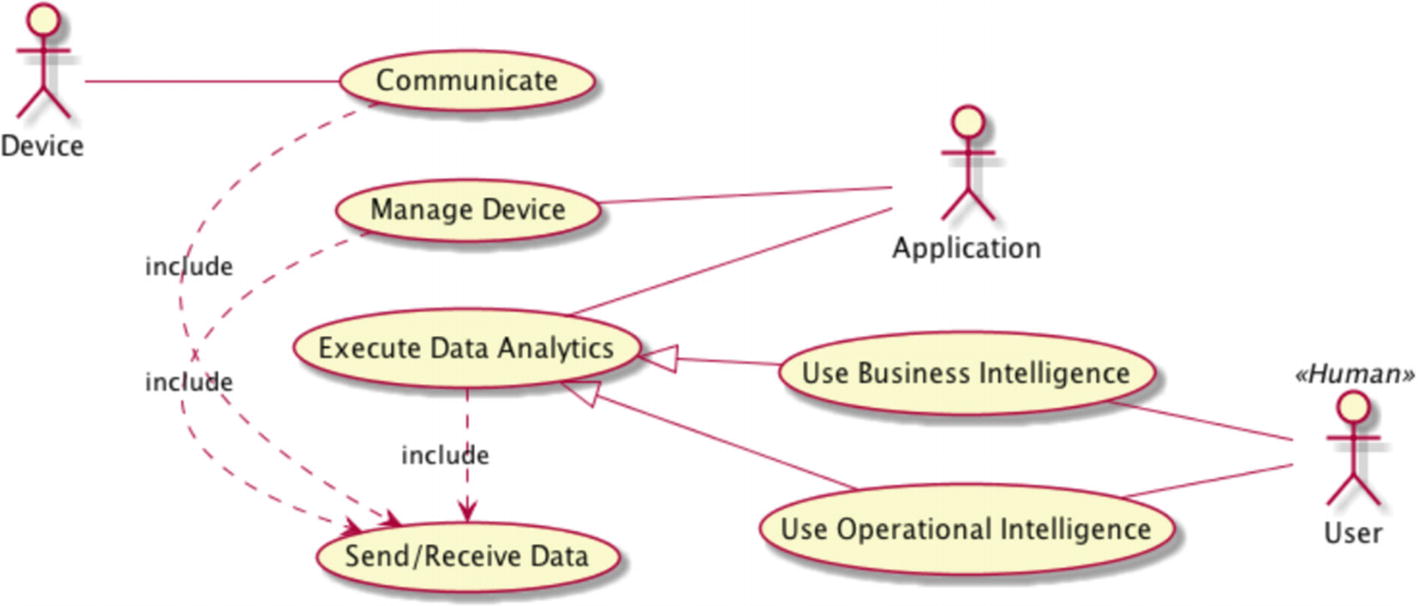
The major use cases and actors in an IoT platform presented as a UML use case diagram (see reference [1] for more information). The usage matrix focuses on use cases and their impact on resources.
Generic Template of a Usage Matrix
UC 1 | UCj | UCn | |
|---|---|---|---|
R 1 | |||
R i | a ij | ||
R m |
Sample Instance of Usage Matrix Template
Row Total | Communicate | Manage Dev. | Exec. Data Analytics | Use Bus. Int. | Use Op. Int. | |
|---|---|---|---|---|---|---|
Network | 615 | 120*1*5=600 | 5*3*1=15 | 0 | 0 | 0 |
Messaging | 700 | 120*1*5=600 | 0 | 20*2*3=100 | 0 | 0 |
Database | 2660 | 0 | 0 | 30*10*3=900 | 40*10*2=800 | 80*3*4=960 |
Column Total | 1200 | 15 | 1000 | 800 | 960 |
The concrete numbers in Table 10-2 are made up and not important. The Send/Receive use case isn’t included explicitly in Table 10-2 because it is part of other use cases. Of course, you may structure the table differently. At any rate, this UC will be associated with the other UC via the dedicated relationship type. Note that the UML extend mechanism isn’t the same as subclassing in Python and we don’t talk here about inheritance. Based on this table, we see that improving the database (possibly using separate technologies for real-time data acquisition and analytics) is most beneficial.
Content of the usage_matrix.py Module
Caution
I advise you to make a copy of the graph before adding visual effects and relabeling nodes (use the copy parameter to perform the operation in place). If you are not careful with the latter, then you may waste lots of time trying to decipher what is going on with the rest of your code (written to use the previous labels). Keep your original graph tidy, as it should serve as a source of truth.

Imagine how much time you would need to spend on this drawing if you weren’t able to utilize NetworkX and Graphviz
For basic drawings, you may rely on the built-in matplotlib engine. However, you shouldn’t use it for more complex drawings because, for example, it is quite tedious to control the sizes and shapes of node boxes in matplotlib. Moreover, as you will encounter later, Graphviz allows you to visualize graphs and run algorithms for controlling layouts. Finding out which resource is the most impacted boils down to calculating the degree of resource nodes by using the in_degree method on a graph (keep in mind the directionality of edges). The only caveat is that you must specify the weight argument (in our case, it would point to the custom weight property of associated edges). In an undirected graph, you would simply use the degree method.
Opposite Quality Attributes
Module signed_graph.py Models the Relationships Between Quality Attributes (see Exercise 10-2)
Partitioning the Model into a Bipartite Graph
An important category of graphs is bipartite graphs, where nodes can be segregated into two disjunct sets L(eft) and R(ight). Edges are only allowed between nodes from disparate sets; that is, no edge may connect two nodes in set L or R. For example, in a recommender system, a set of users and a set of movies form a bipartite graph for the rated relation . It makes no sense for two users or two movies to rate each other. Therefore, there is only an edge between a user and a movie, if that user has rated that movie. The weight of the edge would be the actual rating.
Module bipartite.py Creating a Bipartite Graph from Our Original Multigraph

The Application actor uses all three use cases depicted as a triangle. Therefore, they all have a single common actor. The other two use cases are accessed by the User actor.
Scalable Graph Loading
Thus far, we have constructed our graphs purely by code. This is OK for small examples, but in the real world your network is going to be huge. A better approach is to directly load a graph definition from an external source (such as a text file or database). In this section we will examine how to combine Pandas and NetworkX to produce a graph whose structure is kept inside a CSV file (see also the sidebar “Graph Serialization Formats”).
Graph Serialization Formats
Adjacency (incidence) matrix: This is very similar in structure to our usage matrix, where rows and columns denote nodes. At each intersection of row i and column j there is a value 0 (edge doesn’t exist between nodes i and j) or 1 (edge exists between nodes i and j). You can pass this matrix as an initialization argument when creating a new graph. This matrix isn’t good to specify additional node/edge properties and is very memory hungry. Graphs are typically sparse, so you will have lots of zeros occupying space.
Adjacency list: A separate row exists for each node. Inside a row there are node identifiers of neighbors. This format preserves space, since only existing edges are listed. An isolated node would have an empty row. You cannot define additional properties with this format. NetworkX has a method read_adjlist to read a graph saved as an adjacency list. You can specify the nodetype parameter to convert nodes to a designated type. The create_using parameter is a pointer to the desired factory (for example, you can force NetworkX to load the graph as a multigraph). Text files may contain comments, and these can be skipped by passing the value for the comments parameter.
Edge list: Each row denotes an edge with source and sink node identifiers. You can attach additional items as edge properties (like weight, relation, etc.). It is possible to specify the data types for these properties inside the dedicated read_edgelist method. Note that this format alone cannot represent isolated nodes.
GraphML: This is a comprehensive markup language to express all sorts of graphs (visit http://graphml.graphdrawing.org ). NetworkX has a method read_graphml to read graphs saved in this file format.
Content of the nodes.csv File with a Proper Header Row
edges.edgelist Stores Edges in the Standard Edge List Format
Complete Code to Load Graph from nodes.csv and edges.edgelist
You can also iterate over nonexistent edges in the graph G by invoking nx.non_edges(G). A similar function that returns the non-neighbors of the node n in the graph G is nx.non_neighbors(G, n).
Social Networks
There are many ways to describe social networks, but we will assume in this section that social network means any network of people where both individual characteristics and relationships are important to understand the real world’s dynamics. In data science, we want to produce actionable insights from data. The story always begins with a compelling question. To reason about reality and answer that question, we need a model. It turns out that representing people as nodes and their relationships as edges in a graph is a viable model. There are lots of metrics to evaluate various properties (both local and global) of a graph. From these we can infer necessary rules and synthesize knowledge. Moreover, measures of a graph may be used as features in machine learning systems (for example, to predict new link creations based on known facts from a training dataset).
Module artificial_network.py, Which Demonstrates Some Local and Global Graph Metrics

Apparently, you cannot rely on a single metric to decide about some aspect of a graph
For example, nodes 2, 3, and 4 all have the same closeness centrality. Nonetheless, the betweenness centrality gives precedence to node 2, as it is on more shortest paths in the network. By judiciously selecting and combining different metrics, you may come up with good indicators of a network.
The local clustering coefficient (LCC)
of a node represents the fraction of pairs of the node’s neighbors who are connected. Node 2 has an LCC of 
 is the degree of node 2. LCC embodies people’s tendency to form clusters; in other words, if two persons share a connection, then they tend to become connected, too (a.k.a. triadic closure).
Nodes 2, 3, and 4 are considered central because the maximum shortest path (in our case, measured as the number of hops in a path) to any other node is equal to the radius of the network. The radius of a graph is the minimum eccentricity for all nodes. The eccentricity of a node is the largest distance between this node and all other nodes. The diameter of a graph is the maximum distance between any pair of nodes. Peripheral nodes have eccentricity equal to the diameter. Note that these measures are very susceptible to outliers, in the same way as is the average. By adding a chain of nodes to a network’s periphery, we can easily move the central nodes toward those items. This is why social network are better described with different centrality measures.
The average clustering coefficient is simply a mean of individual clustering coefficients of nodes. The transitivity is another global clustering flag, which is calculated as the ratio of triangles and open triads in a network. For example, the set of nodes 2, 5, and 4 forms an open triad (there is a missing link between nodes 5 and 4 for a triangle). Transitivity puts more weight on high-degree nodes, which is why it is lower than the average clustering coefficient (nodes 2, 3, and 4 as central are heavier penalized for not forming triangles).
The centrality measures try to indicate the importance of nodes in a network. Degree centrality measures the number of connections a node has to other nodes; influential nodes are heavily connected. The closeness centrality says that important nodes are close to other nodes. The betweenness centrality defines a node’s importance by the ratio of shortest paths in a network including the node. There is a similar notion of betweenness centrality for an edge.
karate-network.py Module Exemplifying the Well-Known Karate Club Network (see Exercise 10-3)
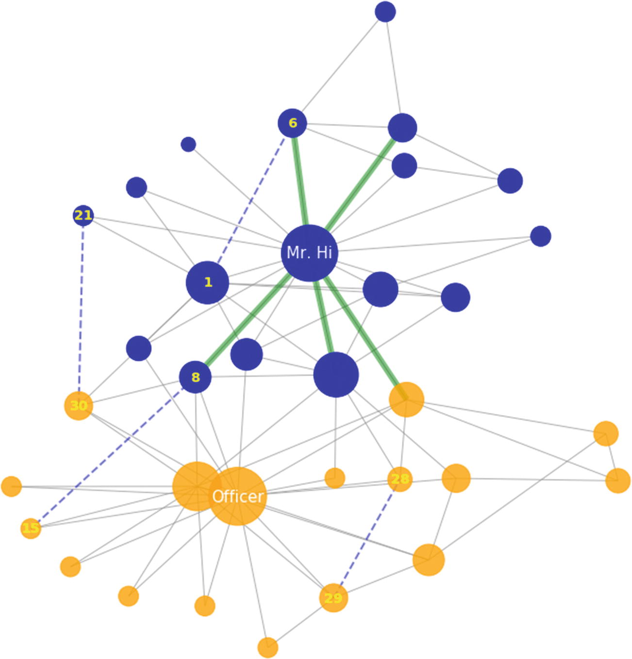
The karate club social network, which clearly emphasizes the split of a club into two parts. The sizes of nodes reflect their degree. The five most important connections are highlighted in green. The dashed lines denote candidate edges. The nodes are colored according to what club they belong to.
Preferential Attachment: Favors nodes with high degree centrality. This is why the score for nodes 1 and 6 is much higher than for the others.
Jaccard Coefficient: The number of common neighbors normalized by the total number of neighbors.
Adamic-Adar Index: Has a logarithm in the denominator that is compared to the Resource Allocation index. For nodes A and B, this index indicates the information flow dispersal level through common neighbors. In a sense, nodes that would like to join tend to have direct communication. If common neighbors have high degree centrality, then such a flow is going to be dissolved.
Community Common Neighbors: The number of common neighbors, with extra points for neighbors from the same community.
Community Resource Allocation: Similar to the Resource Allocation index, but only counts nodes inside the same community. Notice that the candidate edges (9, 15) and (30, 21) have received zero community resources, since they are from different karate clubs.
There are three more real social networks available in NetworkX (as of the time of writing). You may want to experiment with them as we did here. The visualization part can be easily reused.
When you study a social network, it is an interesting option to generate realistic network models. These networks aim to mimic pertinent properties of real-world networks under consideration. There are many network generators available inside NetworkX, including the popular preferential model (which obeys the power law) and the small-world network (which has a relatively high clustering coefficient and short average path length). The latter tries to mimic the six degrees of separation idea. Once you have a model, then you can compare it with observations (samples) from the real world. If the estimated parameters of a model (like the exponent α and constant C in a preferential model) work well to produce networks close to those from the real world, then real-world phenomena may be analyzed by using graph theory and computation. For example, you can train a classifier using network features (like our metrics) to predict probabilities about future connections.
Exercise 10-1. Beautify The Displayed Network, Part 1
Experiment by setting visual properties of edges (we have set some for nodes). For example, you may color relations differently and set the line widths to the weights of relations. As a bonus exercise, try to attach a custom image for actor nodes. This can be done by mixing in HTML content and referencing an image using the img tag.
Exercise 10-2. Beautify The Displayed Network, Part 2
Build on the experience you’ve gained from Exercise 10-1 to visualize a signed graph (like the one we used to model relationships between quality attributes). You may want to display a plus sign or minus sign for each edge as well as color them differently.
You can traverse the edges of an undirected graph G by using the G.edges(data=True) call, which returns all the edges with properties. To display the sign, use the G.edge[node_1][node_2]['sign'] expression, where node_1 and node_2 are node identifiers of this edge.
Exercise 10-3. Generate An Erdös-RÉnyi Network
Read the documentation for the nx.generators.random_graphs.erdos_renyi_graph function to see how to produce this random graph. This model chooses each of the possible edges with probability p, which is a synonym for a binomial graph (since it follows Bernoulli’s probability distribution).
The generated network doesn’t resemble real-world networks (as a matter of fact, the small-world network model doesn’t do a great job in this respect either). Nonetheless, the model is extremely simple, and binomial graphs are used as the basis in graph theory proofs.
Summary
Real-world networks are humungous, so they require more scalable approaches than what has been presented here. One plausible choice is to utilize the Stanford Network Analysis Project (SNAP) framework (visit http://snap.stanford.edu ), which has a Python API, too. Storing huge graphs is also an issue. There are specialized database systems for storing graphs and many more graph formats (most of them are documented and supported by NetworkX). One possible selection for a graph database is Neo4j (see https://neo4j.com/developer/python ).
Graphs are used to judge the robustness of real-world networks (such as the Web, transportation infrastructures, electrical power grids, etc.). Robustness is a quality attribute that indicates how well a network is capable of retaining its core structural properties under failures or attacks (when nodes and/or edges disappear). The basic structural property is connectivity. NetworkX has functions for this purpose (for evaluating both nodes and edges): nx.node_connectivity, nx.minimum_node_cut, nx.edge_connectivity, nx.minimum_edge_cut, and nx.all_simple_paths. The functions are applicable for both undirected and directed graphs. Graphs are also the basis for all sorts of search problems in artificial intelligence.
References
- 1.
Ervin Varga, Draško Drašković, and Dejan Mijić, Scalable Architecture for the Internet of Things: An Introduction to Data-Driven Computing Platforms, O’Reilly, 2018.
- 2.
Ronald C. Read and Robin J. Wilson, An Atlas of Graphs, Oxford University Press, 1999.
- 3.
David Easley and Jon Kleinberg, Networks, Crowds, and Markets: Reasoning About a Highly Connected World, Cambridge University Press, 2010.
- 4.
Michel Rigo, Advanced Graph Theory and Combinatorics, John Wiley & Sons, 2016.