
Let me start by making an analogy between software engineering and data science. Software engineering may be summarized as the application of engineering principles and methods to the development of software. The aim is to produce a dependable software product. In a similar vein, data science may be described as the application of scientific principles and methods to data collection, analysis, and reporting. The goal is to synthesize reliable and actionable insights from data (sometimes referred as data product). To continue with our analogy, the systems/software development life cycle (SDLC) prescribes the major phases of a software development process: project initiation, requirements engineering, design, construction, testing, deployment, and maintenance. The data science process also encompasses multiple phases: project initiation, data acquisition, data preparation, data analysis, reporting, and execution of actions (another “phase” is data exploration, which is more of an all-embracing activity than a stand-alone phase). As in software development, these phases are quite interwoven, and the process is inherently iterative and incremental. An overarching activity that is indispensable in both software engineering and data science (and any other iterative and incremental endeavor) is retrospection, which involves reviewing a project or process to determine what was successful and what could be improved. Another similarity to software engineering is that data science also relies on a multidimensional team or team of teams. A typical project requires domain experts, software engineers specializing in various technologies, and mathematicians (a single person may take different roles at various times). Yet another common denominator with software engineering is a penchant for automation (via programmability of most activities) to increase productivity, reproducibility, and quality. The aim of this chapter is to explain the key concepts regarding data science and put them into proper context.
Main Phases of a Data Science Project
It is a familiar and significant saying that a problem well put is half-solved.
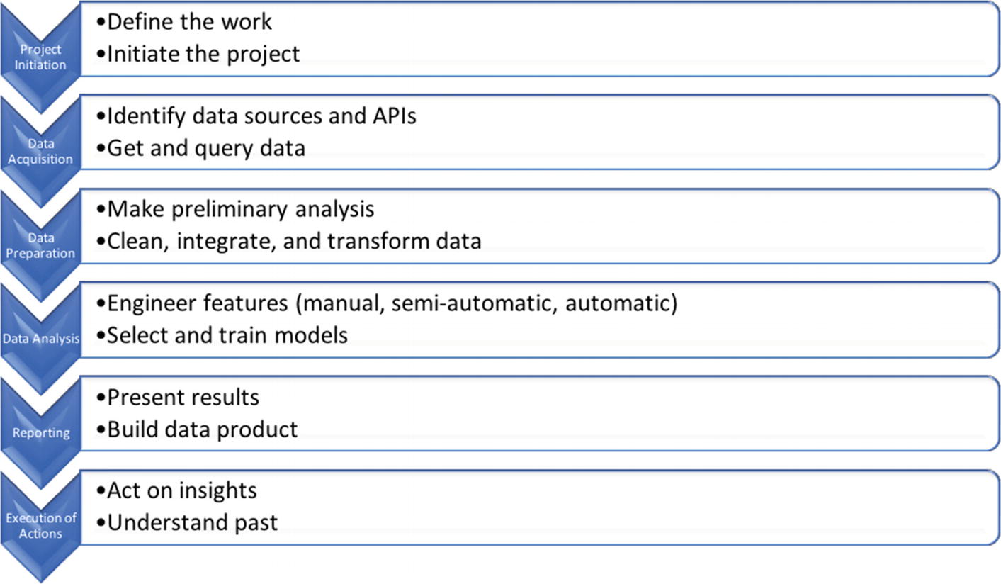
The main phases of a data science project
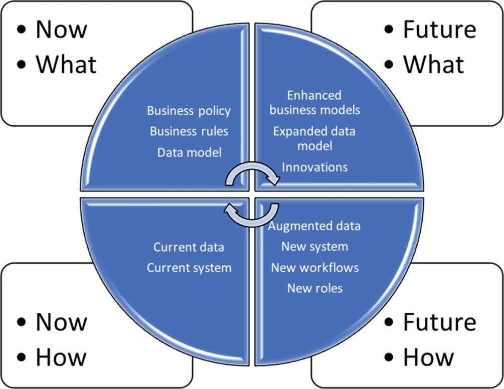
The Brown Cow model adapted for a data science project
The Brown Cow model contains four segments: the How tackles the solution space, the What touches upon the problem space, the Now designates the current situation, while the Future describes the desired state. Each segment designates one specific viewpoint, which helps to avoid confusion among stakeholders. The Brown Cow model incorporates a systematic procedure for transitioning from the current state toward the future, while satisfying the interests of key stakeholders of a project. Without their global consensus, it is very hard to judge the successfulness of the final data product. The next section illustrates this model in a case study.
Brown Cow Model Case Study
Project initiation: Based on symptoms of the disease (vomiting and diarrhea), Dr. Snow properly surmised that it must be caused by an infection carried by something people ate or drank. Prevalent public opinion at that time was that cholera was transmitted by bad smells (a.k.a. miasma theory). According to the Brown Cow model, the Now-How is the existing registry of deaths as well as total confusion regarding what is the root cause of cholera. The Now-What is the prevalent wrong theory of how the disease spreads (with a futile rule to cover your nose and mouth). The Future-What is the new theory of what may cause cholera. The Future-How is the incremental procedure to establish causation between contaminated water and cholera as well as clear advice about what should be the immediate next steps. It is also important to note that this revelation opened up the possibility to further investigate cholera, which eventually led to the discovery of the matching bacteria.
Data engineering 1 (acquisition, preparation, and exploration): Snow recorded the location of each death around the Soho district of London (where the epidemy had emanated) and put everything on a map (as shown in Figure 1-3). He also marked the water pumps on a map to be able to discern patterns. This is a fine example of using visualization in parallel to raw tabular data; exploration most frequently entails some sort of graphics (image, plot, graph, etc.). Exploration as an activity permeates all phases of the data science process, though.

Snow’s original map. Black bars denote deaths. Black discs are pumps. The clustering of death cases around the Broad Street pump is apparent.
Data analysis 1: After Snow carefully examined every case (including important outliers), he established a strong correlation between deaths and the Broad Street pump. He was cautious and resisted establishing causation at this stage. This is a fine example of applying a scientific skillset in working with data (the Web is full of embarrassing stories of correlation being misapplied as causation).
Retrospective: The first milestone was an enabler for the second part.1 Snow had revisited the original plan and prepared the next stage to answer his initial research question. He needed to carry out a randomized control experiment (the best way to assuredly reach causality) and had to use the method of comparison. In a randomized experiment, participants are segregated into two groups: treatment (e.g., those who drank contaminated water) and control (e.g., those who were not exposed to infection). The comparison method seeks to find an association between the applied treatment and observed outcome. It is very important for groups to systematically differ only in that single characteristic that is the criteria for separation. In Snow’s case, this was the water supply received by people in these categories. Luckily, there were two water suppliers whose customers weren’t one-sidedly different in any other aspect except water supply. One supplier delivered clean water upriver from the sewage discharge point, and the other drew its contaminated water below it. The groups were naturally randomized and formed.
Data engineering 2: Snow collected data on all cases of cholera for a broader area of London that were covered by these water suppliers.
Data analysis 2: After a careful analysis, it was evident that people got sick by drinking contaminated water. This was the moment when Snow could safely claim a causal relationship between an infection through contaminated water and cholera.
Reporting: Snow prepared a detailed table showing death rates of people belonging to the two groups. The death rate in the treatment group was ten times higher than that of the control group, so he was confident in his statement.
Action: The authorities removed the handle from the Broad Street pump to prevent further infections, and it proved effective. Further investigations and actions followed this study.
Evidently, this is a compelling data science project from the 19th century. Why, then, is data science such a hot topic nowadays? The answer lurks in the name of the discipline itself (data science). It is popular again due to the vastly different data and concomitant complex problem space(s) embodied by Big Data (see also the sidebar “Big Data Requires Data Scientists”). In the past, data was relatively scarce and data management solutions were much more expensive. Today, we have a data deluge phenomenon that was aptly commented on by John Naisbitt as follows: “We are drowning in information and starving for knowledge.”
Big Data Requires Data Scientists
Big Data, covered in the next section, refers to data at a scale that is difficult to conceptualize. An analogy to help you understand why data scientists are required when designing a Big Data system is that of designing a building. If you want to design your own home, you might be able to draft your own floor plan (or find one on the Internet) and give it to the builder; you don’t need to be an architect. Scale that up to designing a multistory apartment building, then you must be a certified architect, but you can rely on existing resources and tools to complete the design.
Finally, if you’re hired to design the world’s tallest skyscraper or build apartments on an artificial island in the middle of a sea, then you not only must be a certified architect, but also must possess extraordinary knowledge and experience, apply unconventional methods, and devise unique tools. Designing a Big Data system is analogous to designing a skyscraper and requires data scientists with vast knowledge and experience.
Big Data
Volume denotes the sheer amount of data. The assumption is that the vast quantity of data cannot fit on a single machine (not even on disk, let alone in memory), so the data must be distributed over dozens of networked machines. This brings in all sorts of issues related to distributed computing that don’t exist in the case of a single machine.
Variety designates the property of data being organized in various ways. In a classical setup, we presume well-structured data, whose schema is properly documented. Usually such data resides in relational databases. With Big Data, we must also deal with unstructured and semi-structured forms. Nonetheless, all data eventually needs to be aligned and managed in a unified fashion.
Velocity dictates the pace of data changes (arrival of new data, update of existing data, and removal of data). Besides processing data at rest, many times we must handle data changes in real time to avoid any data loss. This kind of data management is known as stream processing. Streams of data may arrive to a system previously trained on historical data and this data combination (historical + real-time) is sometimes called actionable information.
Veracity is about trustworthiness of data. As we amalgamate disparate data sources, we must handle inaccurate, incomplete, and misapplied (sometimes adversary) data.
All these Vs require novel methods, algorithms, and technologies. Also, the complexity and size of the required software systems become larger. These are the principal reasons why data science gets so much attention from both research communities and industry. The next example illustrates these dimensions.
Big Data Example: MOOC Platforms
Differences Between Old and Modern Data Science Projects in Light of Big Data
Snow’s Project | MOOC Platform–Based Project | |
|---|---|---|
Volume | The total impacted population was of a manageable size to be tracked by a single person. | One platform may host hundreds of courses, each potentially having thousands of students. A course is composed of multimedia material as well as content created by participants (comments on the associated discussion forum, exam answers, assignment submissions, etc.). Just to store the data, you need a huge distributed file system. |
Variety | The data was well defined as a set of locations of deaths caused by cholera. | All sorts of data are present: structured course material, unstructured discussion forum stuff, and semi-structured assignment submissions (just to name a few). |
Velocity | The rate of death cases was low enough to be tracked by a person (including visualization effort). | The system experiences an extraordinary amount of activity by its users. Tracking their actions, serving course content, and evaluating exams/assignments require a powerful cloud infrastructure. |
Veracity | The data was absolutely reliable . | On a discussion forum, you can find all kinds of comments. To bring order to that mess, students upvote or downvote posts and course staff also make comments (sometimes simply to endorse a student’s opinion). There are also guidelines about how to name new threads, how to avoid duplication, how to behave politely, etc. |
You may want to read “How Video Production Affects Student Engagement: An Empirical Study of MOOC Videos” (see reference [3]) as an excellent primer for deriving general wisdom from MOOC data (it explores optimal video length range for lectures). The researchers tracked 862 MOOC videos, 120,000+ students, and 6.9 million video-watching sessions on the edX platform. Now compare this MOOC-based project to an even larger system of systems. For example, the Large Hadron Collider (LHC) is the largest data production facility today. If a MOOC platform can be compared to designing a structure, then the LHC is surely an artificial palm island full of expensive houses. Each of the four experiments currently being conducted at the LHC facility produces thousands of gigabytes per second of data, which on a yearly basis results in around 15 petabytes of data. Another data monster is the Internet of Things (IoT), and you can consult reference [4] for more details.
How to Learn Data Science
This is a fundamental topic of data science, since constant learning on all levels (domain, technology, algorithm, programming language, etc.) together with practice are the hallmarks of this profession. Learning data science means gaining knowledge and understanding of data science through study, instruction, and experience. There is an ancient Chinese proverb that emphasizes the advantage of procuring knowledge over sheer consumption: “Give a man a fish and you feed him for a day. Teach a man to fish and you feed him for a lifetime.” This is exactly what we strive to achieve in data science, too; instead of purely devouring current facts, we must synthesize knowledge for the future.
Domain Knowledge Attainment—Example
Pruning of outliers (data points that are inconsistent with the rest of the dataset)
Deleting incomplete observations
Replacing parts of incomplete observations with estimates (for example, by a feature’s mean value)
Removing duplicates (for example, by merging records)
It is not enough to simply remove missing values. Sometimes, blind removal of data may completely distort the result. You must make a judicious decision based on domain knowledge before doing this kind of cleanup.
Suppose that you are a rookie in the field of finance and banking. You are given the task of implementing a function to calculate the growth of money. The inputs are the starting deposit (principal investment) P0 in a bank and the annual rate of interest r (assume it is a fraction between 0 and 1). The bank uses a continuously compounded interest. You also notice a handy formula for this task, P = P0ert, where t is the time in years. The final amount is P (see Exercise 1-2). Easy, right?
Interest rate
Annual interest rate
Compound interest
Continuously compounded interest
The mathematical constant e in the final formula
The interest rate is the percentage by which to increase the current amount. If we start with P0, then we will end up with P1 = P0 + P0r = P0(1 + r). The annual interest rate is what we would get after one year using the previous equation. The compound interest relies on the previously accrued amount. Therefore, after 2 years we would have P2 = P1 + P1r = P1(1 + r) = P0(1 + r)2. Notice how P2 indirectly depends upon P0. If a bank applies this compounding interest multiple times per year (say, with frequency n), then we would use  as our individual interestrate and apply it subsequently n times. All in all, this would result in
 . Finally, the continuous variant of compounding is when we let n → ∞.
This is the point where we must remind ourselves fromcalculus that  . Consequently, we have
 , after substituting
 . If we repeat this compounding over t years, then we get our term from the initially given formula.
This technique of dissecting formulas and studying terminology is one that I always use when learning a new domain. Once you grasp all the concepts and vocabulary of a domain, then it is OK to just accept formulas. Until then, try to split up any novel (to you) descriptions from a domain into constituent parts and analyze them one by one.
Note
If you decide to use a support vector machine (SVM), then you should first read what the kernel method and kernel trick are. Similarly, before you try principal component analysis (PCA), read about eigenvectors, eigenvalues, and orthonormal basis. It is so easy to fool yourself that you’ve achieved something “remarkable” simply because a particular machine learning method has returned positive results.
Programming Skills Attainment—Example
Attempt to Implement a Function to Calculate the Growth of Money
Optimized and Safer Version of Money Growth Calculator
Basic programming knowledge is not enough. You must be acquainted with efficient and powerful data science frameworks and technologies available for Python. Those are the true enablers to tackle Big Data problems. We will see many such frameworks in action throughout this book.
Note
At the very least, you must be proficient in SciPy, a Python-based ecosystem for data science. Moreover, as code complexity grows, you will need to know the principles, rules, and techniques for creating maintainable solutions. For example, if you’ve never heard of defensive programming, then it is time to brush up on your software engineering proficiencies. What would have happened above with p0 and t having different lengths? Where is this checked?
Overview of the Anaconda Ecosystem
Anaconda Distribution is a free ecosystem (includes a sophisticated package and environment manager) of prepackaged libraries for scientific computing and data science in Python. You may download the latest version for your operating system by visiting https://www.anaconda.com/distribution . There is also a paid Enterprise edition, but we will work here with the free Community variant. At the time of this writing, the current version is 5.3, which comes with Python 3.7. You may want to visit first the documentation at https://docs.anaconda.com .
There is also the Miniconda distribution , which contains only the bare minimum Python environment. We will use the full distribution, as we will need many bundled packages. Miniconda is good if you want to have better control over what gets installed, enabling you to save space.
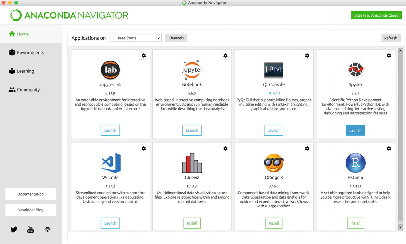
Home page of Anaconda Navigator with the Spyder Launch button selected
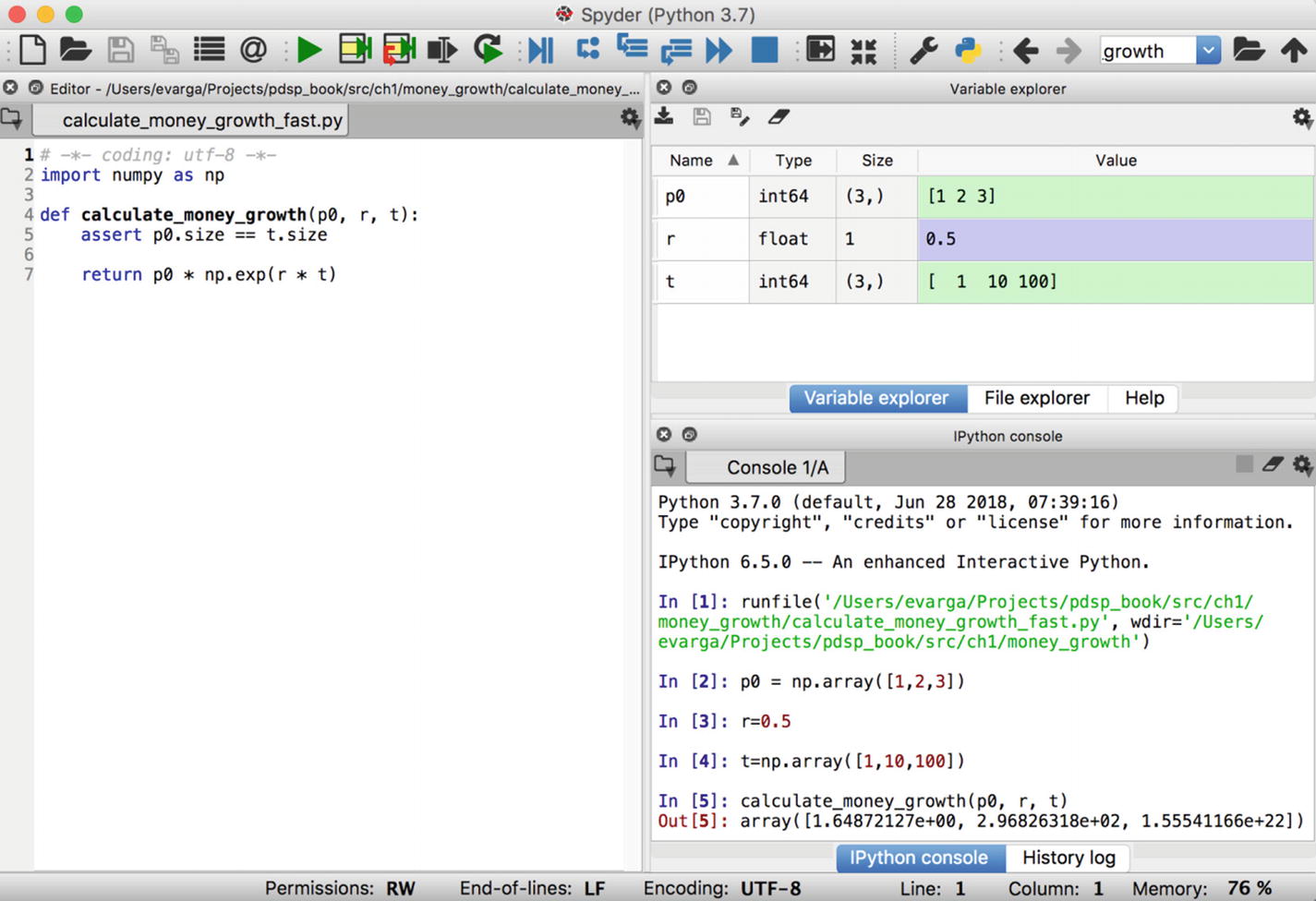
Spyder UI with three main regions
The Editor is located on the left side, the tabbed explorer component is in the upper-right pane (the variable explorer is shown in Figure 1-5), and the IPython console is in the lower-right pane, with expressions to run our fast money growth calculator. The runfile was autogenerated by Spyder after I clicked the Run button (large green arrow) on the toolbar.
If you manage to run the money growth calculator (click the Open Folder button in the toolbar to select and load a file) or evaluate any expression in the IPython console, then all is properly set up. You can also try out the embedded debugger (see the Debug menu, which is the first blue button from the left) by running some code with a configured breakpoint.
Managing Packages and Environments
The first (bold) line shows an easy technique to run shell commands directly within an IPython session and capture their output. I used the list command to enumerate all packages (the central hub for Python packages is accessible at https://pypi.org ). For a list of available conda commands, simply run !conda help (omit the exclamation mark if you execute conda commands from the terminal window).
The fast money growth calculator uses the numpy package, which is preinstalled in my base environment. If you do not have this package, then install it using the conda tool. Now, your solution may stick to one particular set of packages and could refuse to work on another user’s machine (even if all packages are present there, too). Namely, each package has a specific version, and incompatibilities may exist between different versions. Manually ensuring that each application is run with the required set of packages is a daunting task. This is why conda has the concept of an environment. Think about it as a uniquely named namespace that isolates one set of packages from another.
You must activate test, if you want to use it, by executing conda activate test. If you do so, then you will notice that Spyder no longer is available in Anaconda Navigator (it is offered for installation). You may now customize this environment by installing packages into it via conda install. You can customize a passive environment by specifying the --name command-line option. To deactivate an active environment, issue conda deactivate. To remove our test environment, use conda env remove --name test .
The biggest advantage of having a custom environment is that you may export it into a file and put it under version control (together with your project). Anyone may later re-create your environment by using this file. I recommend consulting the conda Cheat Sheet (see https://docs.conda.io/projects/conda/en/latest/user-guide/cheatsheet.html ) for advice on how to perform the most frequent tasks.
Note
If you try to install a new package and receive an error, then it usually helps to update conda to the current version by running conda update conda. Afterward you should retry the installation.
Tip
Beware of creating a new environment by cloning an existing one. Ensure that your custom environment isn’t bloated, which is something you want to avoid.
Sharing and Reproducing Environments
Data science is all about collaboration and teamwork. Sure, environments do help even in a solo arrangement; they endow you with more control over packages, thereby protecting you from inadvertently messing up a working setup. Nonetheless, their true power surfaces when others need to faithfully replicate your work. The conda tool may help here.3
You can share Anaconda-specific files (like notebooks, environments, etc.) in many ways. Anaconda Cloud is one viable option. It allows you to share packages, environments, notebooks, and even whole projects. The latter is still in an experimental stage (at least, this was the case with the anaconda-project package at the time of this writing) but gives you full automation regarding project setup.
Exercise 1-1. Traits of a Data Scientist
Suppose you must prove or disprove the claim that there are integers m and n such that m2 + mn + n2 is a perfect square (see reference [7] for a superb introduction to mathematical reasoning). How would you proceed? (Hint: Think twice before writing a single line of Python code.)
Another situation is that you are asked to write a function to sum the elements of an input floating point array with the highest degree of accuracy. You can neglect the performance implications. What would be the winning approach? If you have managed to solve the problem, then try to explain why the function is behaving as such. Have you ever wondered what causes rounding errors? How is the float data type represented in Python?
A data scientist must possess good analytical skills, be creative, use common sense, and cultivate an inclination to ask Why? questions.
Exercise 1-2. Naming Abstractions
The description and the associated code that follows use strange names P0 and P. In finance there are established terms for these values: present value (PV) and future value (FV), respectively. Alter the associated money growth calculator to use these established terms instead. Do you agree that this simple action has improved comprehensibility?
One of the best ways to check whether your design is sound is by looking at the names of your abstractions. All of them must have a meaningful name. Otherwise, you should rethink the structure of your code. Don’t treat naming as something nobody cares about (your code will be read and maintained by humans).
Summary
Data science is a highly collaborative field that follows an iterative and incremental process. This process consists of many phases, such as planning, data engineering (acquisition, preprocessing, exploration), computational data analysis, reporting, and execution of actions. The aim is to either generate actionable insights from data or explain past phenomena (a.k.a. root cause analysis). A data scientist may play different roles throughout the project, and should possess adequate domain knowledge, math, and software engineering skills. Python is a beloved language of data science because it offers powerful frameworks (besides being a modern and flexible programming language supporting both object-oriented and functional styles).
Anaconda is the recommended ecosystem to develop data science solutions. It bundles all the necessary applications (such as JupyterLab, Spyder, Glueviz, Orange 3, etc.), tools (like the conda manager), and data science packages into a cohesive system. Anaconda also promotes the polyglot programming paradigm, allowing you to implement parts of your project’s portfolio in a multitude of programming languages. It also solves the common problem of crafting reproducible solutions by supporting sophisticated management of packages and environments.
References
- 1.
Suzanne Robertson and James Robertson, “How Now Brown Cow,” The Atlantic Systems Guild, https://www.volere.org/wp-content/uploads/2019/02/howNowBrownCow.pdf , May 2009.
- 2.
Ani Adhikari and John DeNero, Computational and Inferential Thinking: The Foundations of Data Science, https://www.inferentialthinking.com , 2015.
- 3.
Philip J. Guo, Juho Kim, and Rob Rubin, “How Video Production Affects Student Engagement: An Empirical Study of MOOC Videos,” Proceedings of the First ACM Conference on Learning @ Scale Conference (L@S ’14), pp. 41–50 (available at http://pgbovine.net/publications/edX-MOOC-video-production-and-engagement_LAS-2014.pdf ).
- 4.
Ervin Varga, Draško Drašković, and Dejan Mijić, Scalable Architecture for the Internet of Things: An Introduction to Data-Driven Computing Platforms, O’Reilly, 2018.
- 5.
Sinan Ozdemir, Principles of Data Science, Packt Publishing, 2016.
- 6.
David Taylor, “Battle of the Data Science Venn Diagrams,” https://www.kdnuggets.com/2016/10/battle-data-science-venn-diagrams.html , Oct. 6, 2016.
- 7.
Keith Devlin, Introduction to Mathematical Thinking, Keith Devlin, 2012.
- 8.
Joshua Cook, Docker for Data Science: Building Scalable and Extensible Data Infrastructure Around the Jupyter Notebook Server, Apress, 2017.