
SQL Server Big Data Clusters are made up from a variety of technologies all working together to create a centralized, distributed data environment. In this chapter, we are going to look at the various technologies that make up Big Data Clusters through two different views.
First, we are evaluating the more-or-less physical architecture of Big Data Clusters. We are going to explore the use of containers, the Linux operating system, Spark, and the HDFS storage subsystem that make up the storage layer of Big Data Clusters.
In the second part of this chapter, we are going to look at the logical architecture which is made up of four different logical areas. These areas combine several technologies to provide a specific function, or role(s), inside the Big Data Cluster.
Physical Big Data Cluster Infrastructure
The physical infrastructure of Big Data Clusters is made up from containers on which you deploy the major software components. These major components are SQL Server on Linux, Apache Spark, and the HDFS filesystem. The following is an introduction to these infrastructure elements, beginning with containers and moving through the others to provide you with the big picture of how the components fit together.
Containers
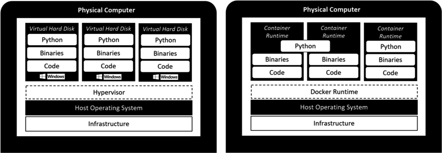
A container is a kind of stand-alone package that contains everything you need to run an application in an isolated or sandbox environment. Containers are frequently compared to virtual machines (VMs) because of the virtualization layers that are present in both solutions. However, containers provide far more flexibility than virtual machines. A notable area of increased flexibility is the area of portability.
One of the main advantages of using containers is that they avoid the implementation of an operating system inside the container. Virtual machines require the installation of their own operating system inside each virtual machine, whereas with containers, the operating system of the host on which the containers are being run is used by each container (through isolated processes). Tools like Docker enable multiple operating systems on a single host machine by running a virtual machine that becomes the host for your containers, allowing you to run a Linux container on Windows, for example.
You can immediately see an advantage here: when running several virtual machines, you also have an additional workload of maintaining the operating system on each virtual machine with patches, configuring it, and making sure everything is running the way it is supposed to be. With containers, you do not have those additional levels of management. Instead, you maintain one copy of the operating system that is shared among all containers.
Another advantage for containers over virtual machines is that containers can be defined as a form of “infrastructure-as-code.” This means you can script out the entire creation of a container inside a build file or image. This means that when you deploy multiple containers with the same image or build file, they are 100% identical. Ensuring 100% identical deployment is something that can be very challenging when using virtual machines, but is easily done using containers.
Virtual machine vs. containers
A final advantage of containers we would like to mention (there are many more to name, however, that would go beyond the scope of this book) is that containers can be deployed as “stateless” applications. Essentially this means that containers won’t change, and they do not store data inside themselves.
Consider, for instance, a situation in which you have a number of application services deployed using containers. In this situation, each of the containers would run the application in the exact same manner and state as the other containers in your infrastructure. When one container crashes, it is easy to deploy a new container with the same build file filling in the role of the crashed container, since no data inside the containers is stored or changed for the time they are running.
The storage of your application data could be handled by other roles in your infrastructure, for instance, a SQL Server that holds the data that is being processed by your application containers, or, as a different example, a file share that stores the data that is being used by the applications inside your containers. Also, when you have a new software build available for your application servers, you can easily create a new container image or build file, map that image or build file to your application containers, and switch between build versions practically on the fly.
SQL Server Big Data Clusters are deployed using containers to create a scalable, consistent, and elastic environment for all the various roles and functions that are available in Big Data Clusters. Microsoft has chosen to deploy all the containers using Kubernetes. Kubernetes is an additional layer in the container infrastructure that acts like an orchestrator. By using Kubernetes (or K8s as it is often called), you get several advantages when dealing with containers. For instance, Kubernetes can automatically deploy new containers whenever it is required from a performance perspective, or deploy new containers whenever others fail.
Because Big Data Clusters are built on top of Kubernetes, you have some flexibility in where you deploy Big Data Clusters. Azure has the ability to use a managed Kubernetes Service (AKS) where you can also choose to deploy Big Data Clusters if you so want to. Other, on-premises options are Docker or Minikube as container orchestrators. We will take a more in-depth look at the deployment of Big Data Clusters inside AKS, Docker, or Minikube in Chapter 3.
Using Kubernetes also introduces a couple of specific terms that we will be using throughout this book. We’ve already discussed the idea and definition of containers. However, Kubernetes (and also Big Data Clusters) also frequently uses another term called “pods.” Kubernetes does not run containers directly; instead it wraps a container in a structure called a pod. A pod combines one or multiple containers, storage resources, networking configurations, and a specific configuration governing how the container should run inside the pod.
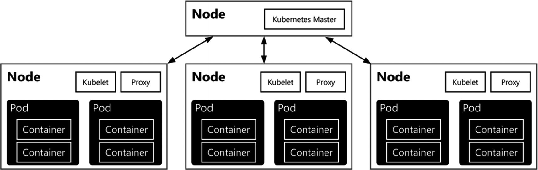
Representation of containers, pods, and nodes in Kubernetes
Generally, pods are used in two manners: a single container per pod or multiple containers inside a single pod. The latter is used when you have multiple containers that need to work together in one way or the other – for instance, when distributing a load across various containers. Pods are also the resource managed to allocate more system resources to containers. For example, to increase the available memory for your containers, a change in the pod’s configuration will result in access to the added memory for all containers inside the pod. On that note, you are mostly managing and scaling pods instead of containers inside a Kubernetes cluster.
Pods run on Kubernetes nodes. A node is the smallest unit of computing hardware inside the Kubernetes cluster. Most of the time, a node is a single physical or virtual machine on which the Kubernetes cluster software is installed, but in theory every machine/device with a CPU and memory can be a Kubernetes node. Because these machines only function as hosts of Kubernetes pods, they can easily be replaced, added, or removed from the Kubernetes architecture, making the underlying physical (or virtual) machine infrastructure very flexible.
SQL Server on Linux
In March 2016, Microsoft announced that the next edition of SQL Server, which turned out to be SQL Server 2017, would be available not only on Windows operating systems but on Linux as well – something that seemed impossible for as long as Microsoft has been building software suddenly became a reality and, needless to say, the entire IT world freaked out.
In hindsight, Microsoft had perfect timing in announcing the strategic decision to make one of its flagship products available on Linux. The incredible adaptation of new technologies concerning containers, which we discussed in the previous section, was mostly based on Linux distributions. We believe that without the capability’s containers, and thus the Linux operating system those containers provide, there would never have been a SQL Server Big Data Cluster product.
Thankfully Microsoft pushed through on their adoption of Linux, and with the latest SQL Server 2019 release, many of the issues that plagued the SQL Server 2017 release on Linux are now resolved and many capabilities that were possible on the Windows version have been brought to Linux as well.
So how did Microsoft manage to run an application designed for the Windows operating system on Linux? Did they rewrite all the code inside SQL Server to make it run on Linux? As it turns out, things are far more complicated than a rewrite of the code base to make it Linux compatible.
To make SQL Server run on Linux, Microsoft introduced a concept called a Platform Abstraction Layer (or PAL for short). The idea of a PAL is to separate the code needed to run, in this case, SQL Server from the code needed to interact with the operating system. Because SQL Server has never run on anything other than Windows, SQL Server is full of operating system references inside its code. This would mean that getting SQL Server to run on Linux would end up taking enormous amounts of time because of all the operating system dependencies.
Drawbridge is a research prototype of a new form of virtualization for application sandboxing. Drawbridge combines two core technologies: First, a picoprocess, which is a process-based isolation container with a minimal kernel API surface. Second, a library OS, which is a version of Windows enlightened to run efficiently within a picoprocess.
The main part that attracted the SQL Server team to the Drawbridge project was the library OS technology. This new technology could handle a very wide variety of Windows operating system calls and translate them to the operating system of the host, which in this case is Linux.
Now, the SQL Server team did not adapt the Drawbridge technology one-on-one as there were some challenges involved with the research project. One of the challenges was that the research project was officially completed which means that there was no support on the project. Another challenge was a large overlap of technologies inside the SQL Server OS (SOS) and Drawbridge. Both solutions, for example, have their own functionalities to handle memory management and threading/scheduling.
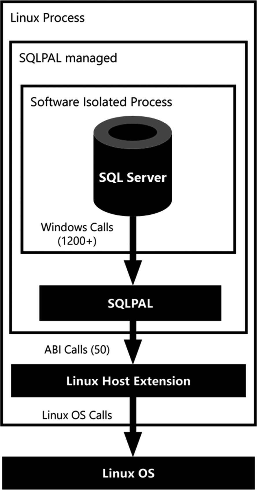
Interaction between the various layers of SQL Server on Linux
There is a lot more information available on various Microsoft blogs that cover more of the functionality and the design choices of the SQLPAL. If you want to know more about the SQLPAL, or how it came to life, we would recommend the article “SQL Server on Linux: How? Introduction” available at https://cloudblogs.microsoft.com/sqlserver/2016/12/16/sql-server-on-linux-how-introduction/.
Next to the use of containers, SQL Server 2019 on Linux is at the heart of the Big Data Cluster product. Almost everything that happens inside the Big Data Cluster in terms of data access, manipulation, and the distribution of queries occurs through SQL Server on Linux instances which are running inside containers.
When deploying a Big Data Cluster, the deployment script will take care of the full SQL Server on Linux installation inside the containers. This means there is no need to manually install SQL Server on Linux, or even to keep everything updated. All of this is handled by the Big Data Cluster deployment and management tools.
Spark
With the capability to run SQL Server on Linux, a load of new possibilities became available regarding the integration of SQL Server with various open source and Linux-based products and technologies. One of the most exciting combinations that became a reality inside SQL Server Big Data Clusters is the inclusion of Apache Spark.
SQL Server is a platform for relational databases. While technologies like PolyBase enable the reading of nonrelational data (or relational data from another relational platform like Oracle or Teradata) into the relational format SQL Server requires, in its heart SQL Server never dealt much with unstructured or nonrelational data. Spark is a game changer in this regard.
The inclusion of Spark inside the product means you can now easily process and analyze enormous amounts of data of various types inside your SQL Server Big Data Cluster using either Spark or SQL Server, depending on your preferences. This ability to process large volumes of data allows for maximum flexibility and makes parallel and distributed processing of datasets a reality.
Apache Spark was created at the University of Berkeley in 2009 mostly as an answer to the limitations of a technology called MapReduce. The MapReduce programming model was developed by Google and was the underlying technology used to index all the web pages on the Internet (and might be familiar to you in the Hadoop MapReduce form). MapReduce is best described as a framework for the parallel processing of huge datasets using a (large) number of computers known as nodes. This parallel processing across multiple nodes is important since datasets reached such sizes that they could no longer efficiently be processed by single machines. By spreading the work, and data, across multiple machines, parallelism could be achieved which results in the faster processing of those big datasets.
- 1.
Input splits
The input to a MapReduce job is split into logical distribution of the data stored in file blocks. The MapReduce job calculates which records fit inside a logical block, or “splits,” and decides on the number of mappers that are required to process the job.
- 2.
Mapping
During mapping our query is being performed on each of the “splits” separately and produces the output for the specific query on the specific split. The output is always a form of key/value pairs that are returned by the mapping process.
- 3.
Shuffling
The shuffling process is, simply said, the process of sorting and consolidating the data that was returned by the mapping process.
- 4.
Reducing
The final step, reducing, aggregates the results returned by the shuffling process and returns a single output.
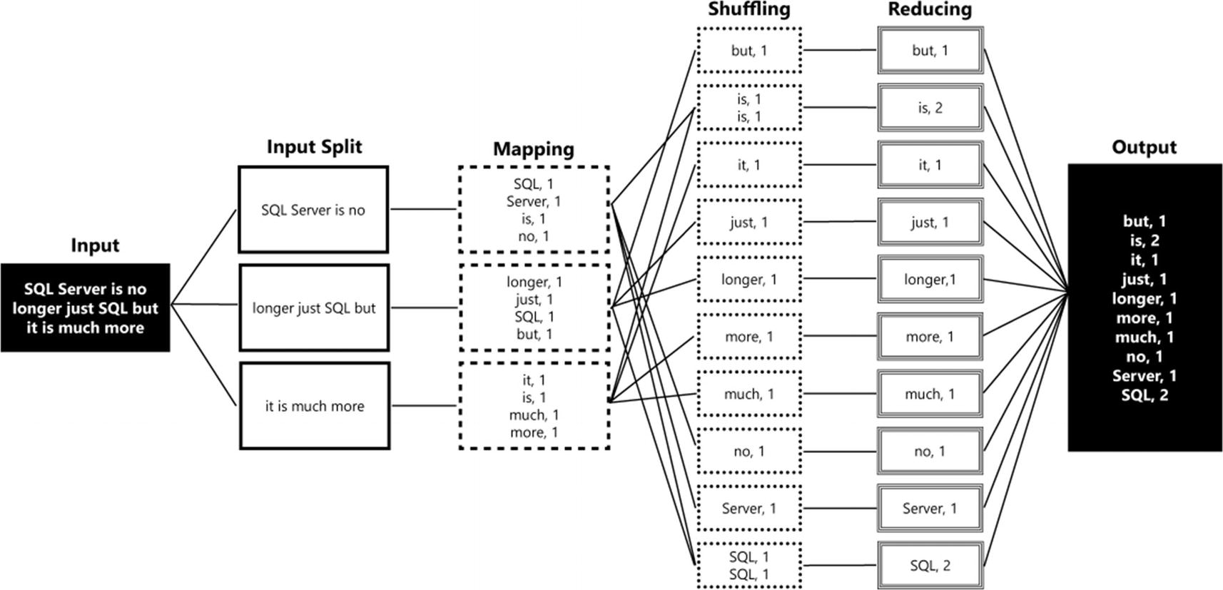
MapReduce example job
What happens in the example is that the dataset that contains the input for our job (the sentence “SQL Server is no longer just SQL but is also much more”) is split up into three different splits. These splits are processed in the mapping phase, resulting in the word counts for each split. The results are sent to the shuffling step which places all the results in order. Finally, the reduce step calculates the total occurrences for each individual word and returns it as the final output.
As you can see from the (simple) example in Figure 2-4, MapReduce is very efficient in distributing and coordinating the processing of data across a parallel environment. However, the MapReduce framework also had a number of drawbacks, the most notable being the difficulty of writing large programs that require multiple passes over the data (for instance, machine learning algorithms). For each pass over a dataset, a separate MapReduce job had to be written, each one loading the data it required from scratch again. Because of this, and the way MapReduce accesses data, processing data inside the MapReduce framework can be rather slow.
Spark was created to address these problems and make big data analytics more flexible and better performing. It does so by implementing in-memory technologies that allow sharing of data between processing steps and by allowing ad hoc data processing instead of having to write complex MapReduce jobs to process data. Also, Spark supports a wide variety of libraries that can enhance or expand the capabilities of Spark, like processing streaming data or performing machine learning tasks, and even query data through the SQL language.
Spark looks and acts a lot like the MapReduce framework in that Spark is also a coordinator, and manager, of tasks that process data. Just like MapReduce, Spark uses workers to perform the actual processing of data. These workers get told what to do through a so-called Spark application which is defined as a driver process. The driver process is essentially the heart of a Spark application, and it keeps track of the state of your Spark application, responds to input or output, and schedules and distributes work to the workers. One advantage of the driver process is that it can be “driven” from different programming languages, like Python or R, through language APIs. Spark handles the translation of the commands in the various languages to Spark code that gets processed on the workers.
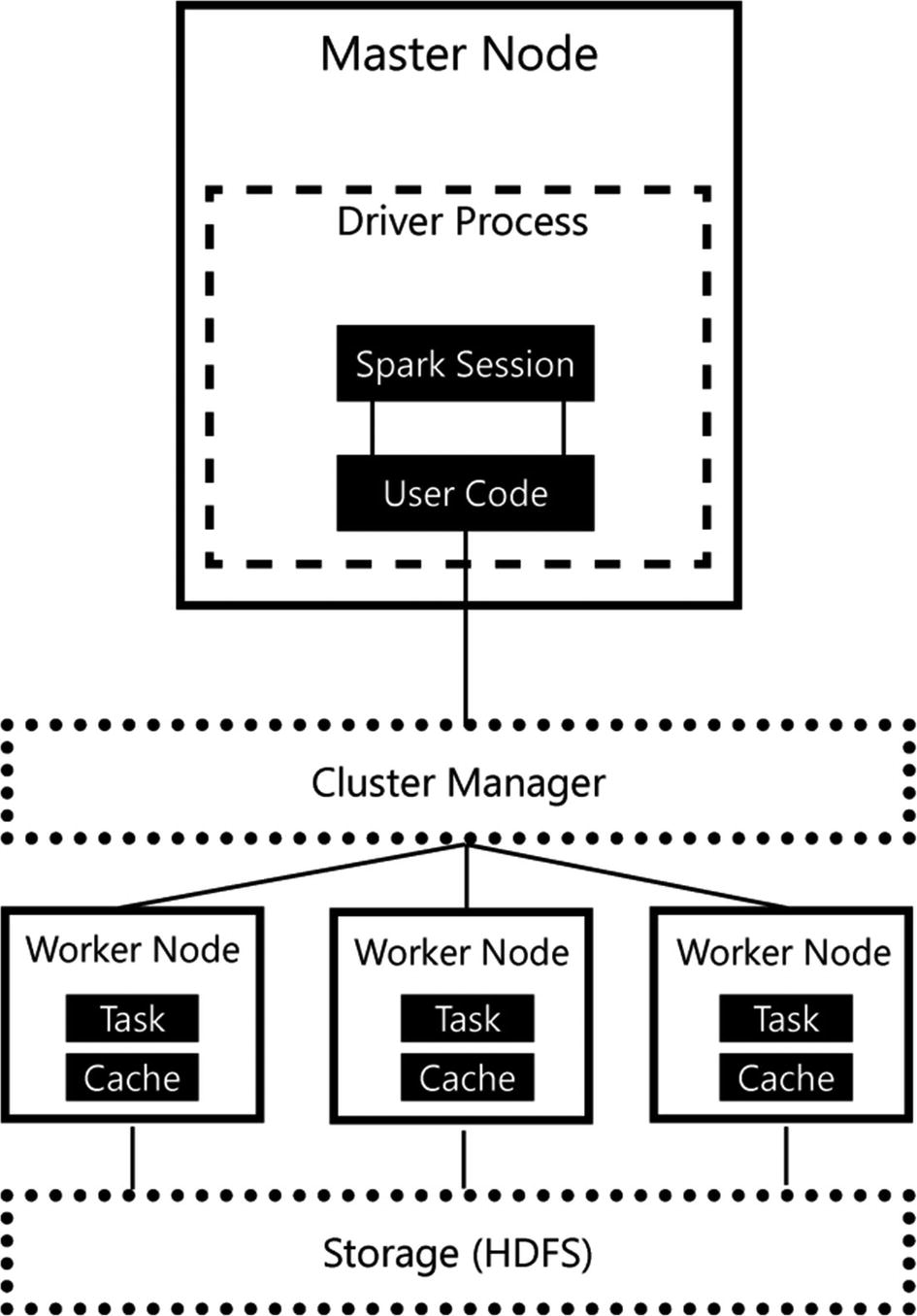
There is a reason why we specifically mentioned the word “logical” in connection with Spark’s architecture. Even though Figure 2-5 implies that worker nodes are separate machines that are part of a cluster, it is in fact possible in Spark to run as many worker nodes on a machine as you please. As a matter of fact, both the driver process and worker nodes can be run on a single machine in local mode for testing and development tasks.
Figure 2-5 also shows how a Spark application coordinates work across the cluster. The code you write as a user is translated by the driver process to a language your worker nodes understand; it distributes the work to the various worker nodes which handle the data processing. In the illustration, we specifically highlighted the cache inside the worker node. The cache is one part of why Spark is so efficient in performing data processing since it can store intermediate processing results in the memory of the node, instead of on disk like, for example, Hadoop MapReduce.
Inside SQL Server Big Data Clusters, Spark is included inside a separate container that shares a pod together with a SQL Server on Linux container.
One thing we haven’t touched upon yet is the way nonrelational data outside SQL Server is stored inside Big Data Clusters. If you are familiar with Spark- or Hadoop-based big data infrastructure, the next section should not come as a surprise.
HDFS
HDFS, or the Hadoop Distributed File System, is the primary method of storing data inside a Spark architecture. HDFS has many advantages in how it stores and processes data stored on the filesystem, like fault tolerance and distribution of data across multiple nodes that make up the HDFS cluster.
The way HDFS works is it breaks up the data in separate blocks (called chunks) and distributes them across the nodes that make up the HDFS environment when data is stored inside the filesystem. The chunks, with a default size of 64 MB, are then replicated across multiple nodes to enable fault tolerance. If one node fails, copies of data chunks are also available on other nodes, which means the filesystem can easily recover from data loss on single nodes.
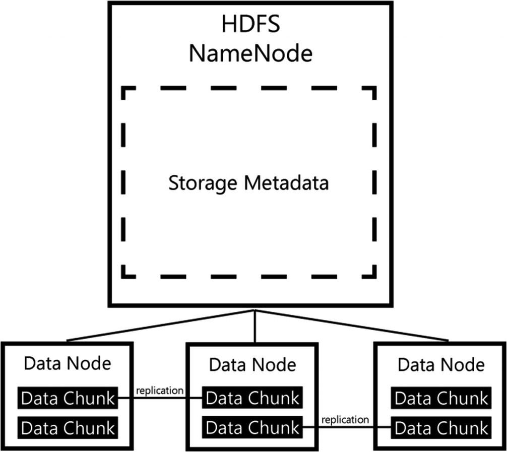
HDFS architecture
In many aspects, HDFS mirrors the architecture of Hadoop and, in that sense, of Spark as we have shown in the previous section. Because of the distributed nature of data stored inside the filesystem, it is possible, and in fact expected, that data is distributed across the nodes that also handle the data processing inside the Spark architecture. This distribution of data brings a tremendous advantage in performance; since data resides on the same node that is responsible for the processing of that data, it is unnecessary to move data across a storage architecture. With the added benefit of data caching inside of the Spark worker nodes, data can be processed very efficiently indeed.
One thing that requires pointing out is that unlike with Hadoop, Spark is not necessarily restricted to data residing in HDFS. Spark can access data that is stored in a variety of sources through APIs and native support. Examples include various cloud storage platforms like Azure Blob Storage or relational sources like SQL Server.
Tying the Physical Infrastructure Parts Together
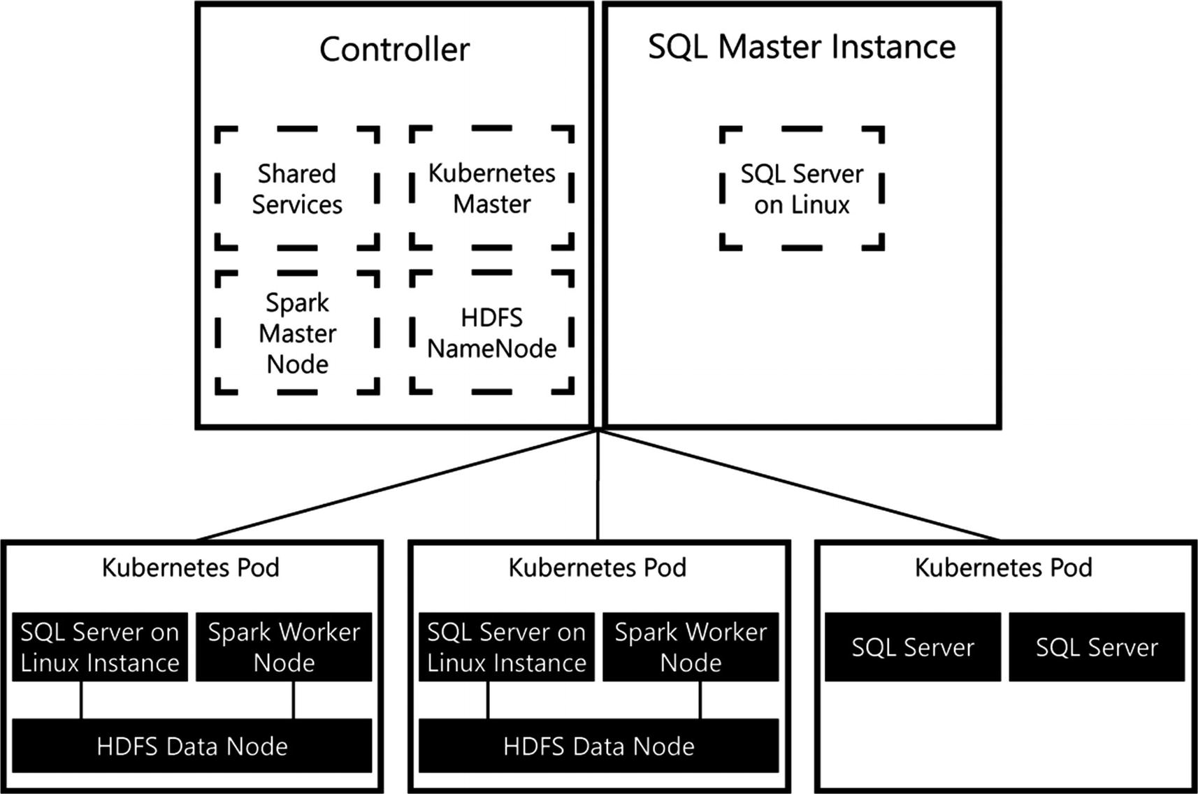
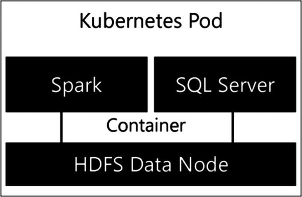
SQL Server Big Data Cluster architecture with Spark, HDFS, and Kubernetes
As you can see from Figure 2-7, SQL Server Big Data Clusters combine a number of different roles inside the containers that are deployed by Kubernetes. Placing both SQL Server and Spark together in a container with the HDFS Data Node allows both products to access data that is stored inside HDFS in a performance-optimized manner. In SQL Server this data access will occur through PolyBase, while Spark can natively query data residing in HDFS.
The architecture in Figure 2-7 also gives us two distinct different paths in how we can process and query our data. We can decide on storing data inside a relational format using the SQL Server instances available to us, or we can use the HDFS filesystem and store (nonrelational) data in it. When the data is stored in HDFS, we can access and process that data in whichever manner we prefer. If your users are more familiar with writing T-SQL queries to retrieve data, you can use PolyBase to bring the HDFS-stored data inside SQL Server using an external table. On the other hand, if users prefer to use Spark, they can write Spark applications that access the data directly from HDFS. Then if needed, users can invoke a Spark API to combine relational data stored in SQL Server with the nonrelational data stored in HDFS.
Logical Big Data Cluster Architecture
As mentioned in the introduction of this chapter, Big Data Clusters can be divided into four logical areas. Consider these areas as a collection of various infrastructure and management parts that perform a specific function inside the cluster. Each of the areas in turn has one or more roles it performs. For instance, inside the Data Pool area, there are two roles: the Storage Pool and the SQL Data Pool.
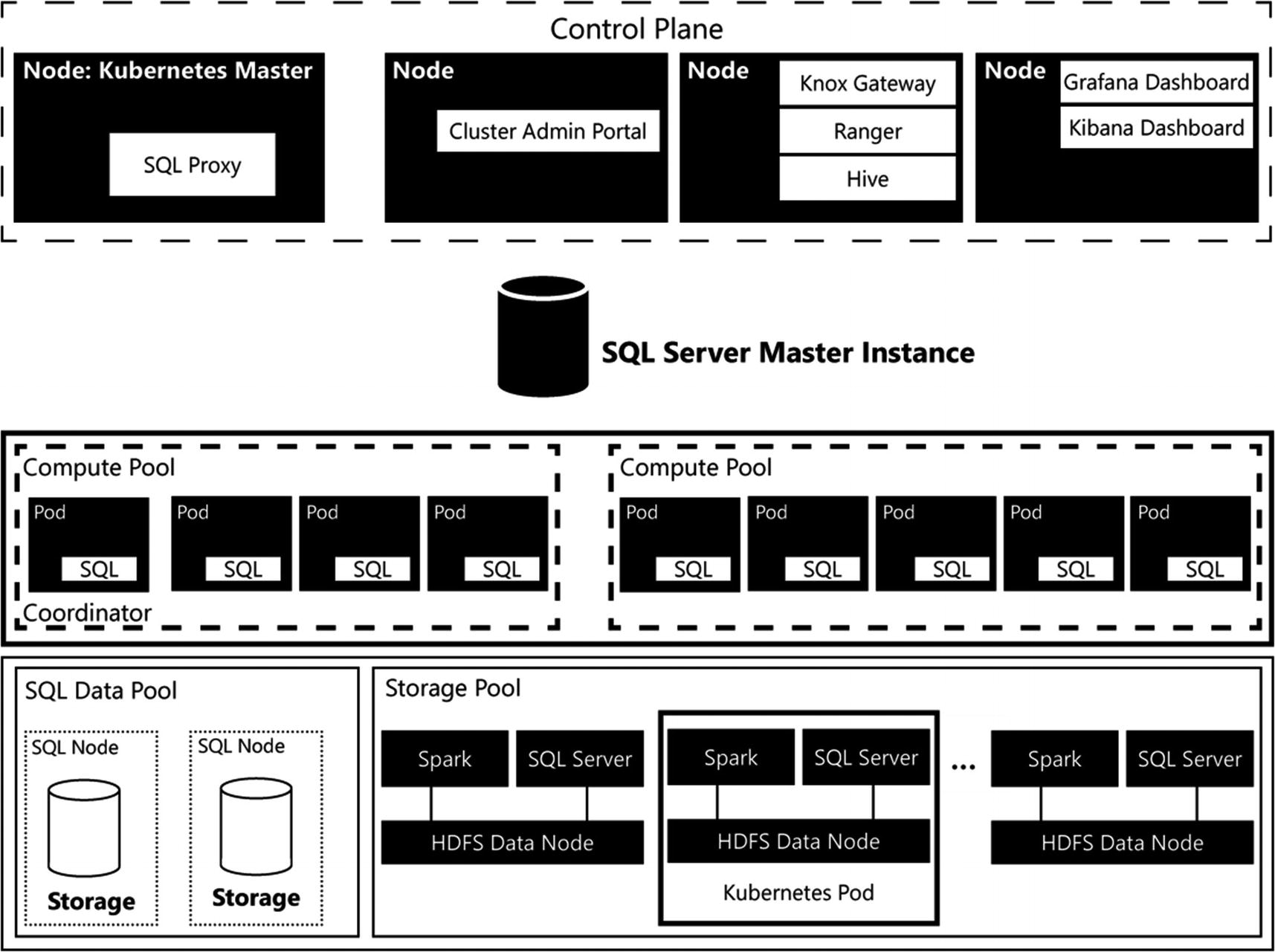
Big Data Cluster architecture
You can immediately infer the four logical areas: the Control area (which internally is named the Control Plane) and the Compute, Data, and App areas. In the following sections, we are going to dive into each of these logical areas individually and describe their function and what roles are being performed in it. Before we start taking a closer look at the Control Plane, you might have noticed there is an additional role displayed in Figure 2-8, the SQL Server Master Instance.
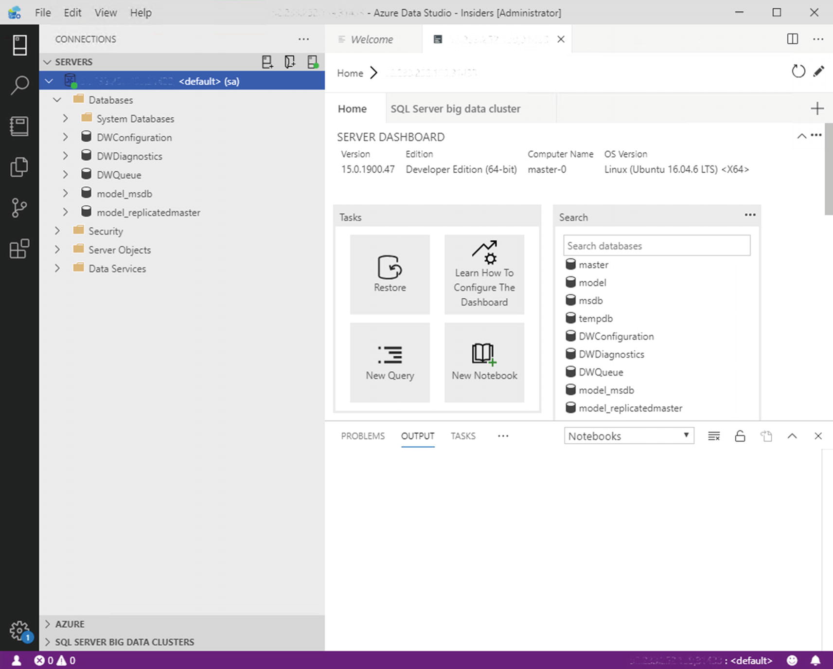
Connection to the SQL Server master instance through Azure Data Studio
In many ways the SQL Server master instance acts like a normal SQL Server instance. You can access it and browse through the instance using Azure Data Studio and query the system and user databases that are stored inside of it. One of the big changes compared to a traditional SQL Server instance is that the SQL Server master instance will distribute your queries across all SQL Server nodes inside the Compute Pool(s) and access data that is stored, through PolyBase, on HDFS inside the Data Plane.
By default, the SQL Server master instance also has Machine Learning Services enabled. This allows you to run in-database analytics using R, Python, or Java straight from your queries. Using the data virtualization options provided in SQL Server Big Data Cluster, Machine Learning Services can also access nonrelational data that is stored inside the HDFS filesystem. This means that your data analysists or scientists can choose to use either Spark or SQL Server Machine Learning Services to analyze, or operationalize, the data that is stored in the Big Data Cluster. We are going to explore these options in a more detailed manner in Chapter 7.
Control Plane
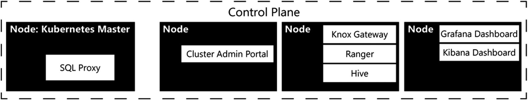
Big Data Cluster Control Plane
In terms of managing Big Data Clusters, we are going to discuss the various management tools we can use to manage Big Data Clusters in Chapter 3.
Next to providing a centralized location where you can perform all your Big Data Cluster management tasks, the Control Plane also plays a very important part in the coordination of tasks to the underlying Compute and Data areas. The access to the Control Plane is available through the controller endpoint.
The controller endpoint is used for the Big Data Cluster management in terms of deployment and configuration of the cluster. The endpoint is accessed through REST APIs, and some services inside the Big Data Cluster, as well as the command-line tool we use to deploy and configure our Big Data Cluster, access those APIs.
You are going to get very familiar with the controller endpoint in the next chapter, in which we will deploy and configure a Big Data Cluster using azdata .
Compute Area
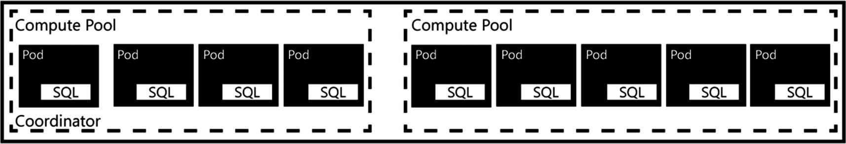
Big Data Cluster Compute area
The main advantage of having a Compute Pool is that it opens up options to distribute, or scale out, queries across multiple nodes inside each Compute Pool, boosting the performance of PolyBase queries.
By default, you will have access to a single Compute Pool inside the Compute logical area. You can, however, add multiple Compute Pools in situations where, for instance, you want to dedicate resources to access a specific data source. All management and configuration of each Kubernetes Pod inside the Compute Pool is handled by the SQL Server Master Instance.
Data Area
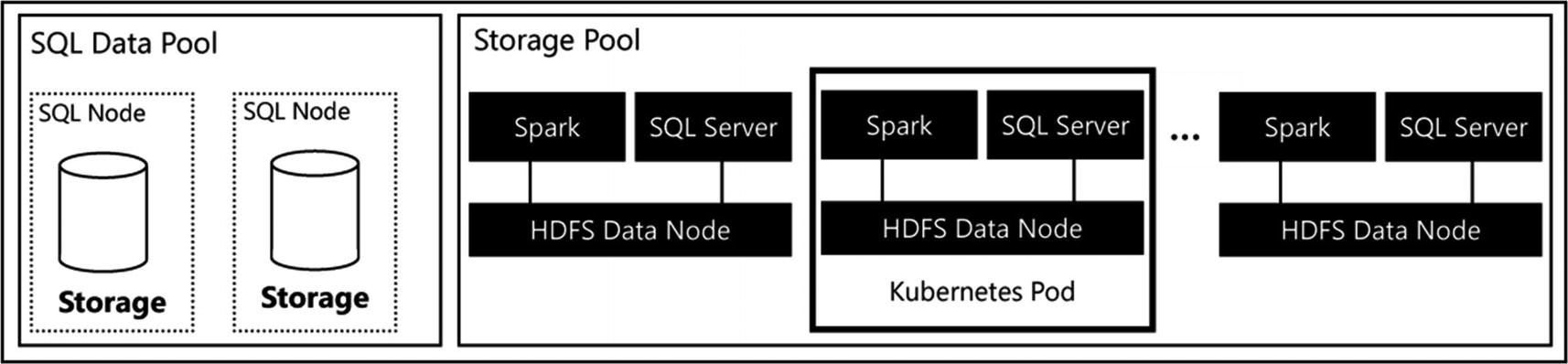
Data Plane architecture
Storage Pool
Storage Node inside the Storage Pool
The HDFS Data Nodes are combined into a single HDFS cluster that is present inside your Big Data Cluster. The main function of the Storage Pool is to provide a HDFS storage cluster to store data on what is ingested through, for instance, Spark. By creating a HDFS cluster, you basically have access to a data lake inside the Big Data Cluster where you can store a wide variety of nonrelational data, like Parquet or CSV files.
The HDFS cluster automatically arranges data persistence since the data you import into the Storage Pool is automatically spread across all the Storage Nodes inside the Storage Pool. This spreading of data across nodes also allows you to quickly analyze large volumes of data, since the load of analysis is spread across the multiple nodes. One advantage of this architecture is that you can either use the local storage present in the Data Node or add your own persistent storage subsystem to the nodes.
Just like the Compute Pool, the SQL Server instances that are present in the Storage Node are accessed through the SQL Server master instance. Because the Storage Node combines SQL Server and Spark, all data residing on or managed by the Storage Nodes can also be directly accessed through Spark. That means you do not have to use PolyBase to access the data inside the HDFS environment. This allows more flexibility in terms of data analysis or data engineering.
SQL Data Pool
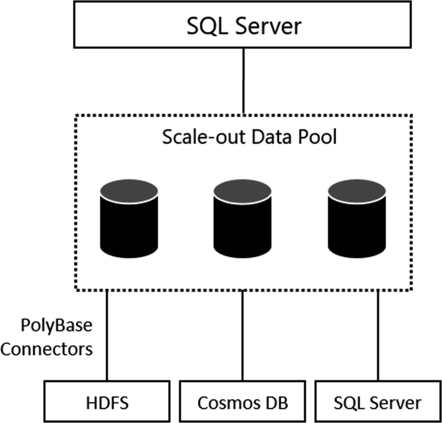
Scaling and caching of external data sources inside the SQL Data Pool
The main role of the SQL Data Pool is to optimize access to external sources using PolyBase. The SQL Data Pool can than partition and cache data from those external sources inside the SQL Server instances and ultimately provide parallel and distributed queries against the external data sources. To provide this parallel and distributed functionality, datasets inside the SQL Data Pool are divided into shards across the nodes inside the SQL Data Pool.
Summary
In this chapter, we’ve looked at the SQL Server Big Data Cluster architecture in two manners: physical and logical. In the physical architecture, we focused on the technologies that make up the Big Data Cluster like containers, SQL-on-Linux and Spark. In the logical architecture, we discussed the different logical areas inside Big Data Clusters that each perform a specific role or task inside the cluster.
For each of the technologies used in Big Data Clusters, we gave a brief introduction in its origins as well as what part the technology plays inside Big Data Clusters. Because of the wide variety of technologies and solutions used in SQL Server Big Data Clusters, we tried to be as thorough as possible in describing the various technologies; however, we also realize we cannot describe each of these technologies in as much detail as we would have liked. For instance, just on Spark, there have been dozens of books written and published describing how it works and how you can leverage the technology. In the area of SQL-on-Linux, HDFS, and Kubernetes, the situation isn’t much different. For that reason, it is best to consider this chapter a simple and brief introduction to the technology or solution, enough to get you started on understanding and using SQL Server Big Data Clusters.