
Chapter 3. K-Nearest Neighbors
Have you ever bought a house before? If you’re like a lot of people around the world, the joy of owning your own home is exciting, but the process of finding and buying a house can be stressful. Whether we’re in a economic boom or recession, everybody wants to get the best house for the most reasonable price.
But how would you go about buying a house? How do you appraise a house? How does a company like Zillow come up with their Zestimates? We’ll spend most of this chapter answering questions related to this fundamental concept: distance-based approximations.
First we’ll talk about how we can estimate a house’s value. Then we’ll discuss how to classify houses into categories such as “Buy,” “Hold,” and “Sell.” At that point we’ll talk about a general algorithm, K-Nearest Neighbors, and how it can be used to solve problems such as this. We’ll break it down into a few sections of what makes something near, as well as what a neighborhood really is (i.e., what is the optimal K for something?).
How Do You Determine Whether You Want to Buy a House?
This question has plagued many of us for a long time. If you are going out to buy a house, or calculating whether it’s better to rent, you are most likely trying to answer this question implicitly. Home appraisals are a tricky subject, and are notorious for drift with calculations. For instance on Zillow’s website they explain that their famous Zestimate is flawed. They state that based on where you are looking, the value might drift by a localized amount.
Location is really key with houses. Seattle might have a different demand curve than San Francisco, which makes complete sense if you know housing! The question of whether to buy or not comes down to value amortized over the course of how long you’re living there. But how do you come up with a value?
How Valuable Is That House?
Things are worth as much as someone is willing to pay.
Old Saying
Note
Valuing a house is tough business. Even if we were able to come up with a model with many endogenous variables that make a huge difference, it doesn’t cover up the fact that buying a house is subjective and sometimes includes a bidding war. These are almost impossible to predict. You’re more than welcome to use this to value houses, but there will be errors that take years of experience to overcome.
A house is worth as much as it’ll sell for. The answer to how valuable a house is, at its core, is simple but difficult to estimate. Due to inelastic supply, or because houses are all fairly unique, home sale prices have a tendency to be erratic. Sometimes you just love a house and will pay a premium for it.
But let’s just say that the house is worth what someone will pay for it. This is a function based on a bag of attributes associated with houses. We might determine that a good approach to estimating house values would be:
Equation 3-1. House value
This model could be found through regression (which we’ll cover in Chapter 5) or other approximation algorithms, but this is missing a major component of real estate: “Location, Location, Location!” To overcome this, we can come up with something called a hedonic regression.
Hedonic Regression
Note
You probably already know of a frequently used real-life hedonic regression: the CPI index. This is used as a way of decomposing baskets of items that people commonly buy to come up with an index for inflation.
Economics is a dismal science because we’re trying to approximate rational behaviors. Unfortunately we are predictably irrational (shout-out to Dan Ariely). But a good algorithm for valuing houses that is similar to what home appraisers use is called hedonic regression.
The general idea with hard-to-value items like houses that don’t have a highly liquid market and suffer from subjectivity is that there are externalities that we can’t directly estimate. For instance, how would you estimate pollution, noise, or neighbors who are jerks?
To overcome this, hedonic regression takes a different approach than general regression. Instead of focusing on fitting a curve to a bag of attributes, it focuses on the components of a house. For instance, the hedonic method allows you to find out how much a bedroom costs (on average).
Take a look at the Table 3-1, which compares housing prices with number of bedrooms. From here we can fit a naive approximation of value to bedroom number, to come up with an estimate of cost per bedroom.
| Price (in $1,000) | Bedrooms |
|---|---|
$899 |
4 |
$399 |
3 |
$749 |
3 |
$649 |
3 |
This is extremely useful for valuing houses because as consumers, we can use this to focus on what matters to us and decompose houses into whether they’re overpriced because of bedroom numbers or the fact that they’re right next to a park.
This gets us to the next improvement, which is location. Even with hedonic regression, we suffer from the problem of location. A bedroom in SoHo in London, England is probably more expensive than a bedroom in Mumbai, India. So for that we need to focus on the neighborhood.
What Is a Neighborhood?
The value of a house is often determined by its neighborhood. For instance, in Seattle, an apartment in Capitol Hill is more expensive than one in Lake City. Generally speaking, the cost of commuting is worth half of your hourly wage plus maintenance and gas,1 so a neighborhood closer to the economic center is more valuable.
But how would we focus only on the neighborhood?
Theoretically we could come up with an elegant solution using something like an exponential decay function that weights houses closer to downtown higher and farther houses lower. Or we could come up with something static that works exceptionally well: K-Nearest Neighbors.
K-Nearest Neighbors
What if we were to come up with a solution that is inelegant but works just as well? Say we were to assert that we will only look at an arbitrary amount of houses near to a similar house we’re looking at. Would that also work?
Surprisingly, yes. This is the K-Nearest Neighbor (KNN) solution, which performs exceptionally well. It takes two forms: a regression, where we want a value, or a classification. To apply KNN to our problem of house values, we would just have to find the nearest K neighbors.
The KNN algorithm was originally introduced by Drs. Evelyn Fix and J. L. Hodges Jr, in an unpublished technical report written for the U.S. Air Force School of Aviation Medicine. Fix and Hodges’ original research focused on splitting up classification problems into a few subproblems:
-
Distributions F and G are completely known.
-
Distributions F and G are completely known except for a few parameters.
-
F and G are unknown, except possibly for the existence of densities.
Fix and Hodges pointed out that if you know the distributions of two classifications or you know the distribution minus some parameters, you can easily back out useful solutions. Therefore, they focused their work on the more difficult case of finding classifications among distributions that are unknown. What they came up with laid the groundwork for the KNN algorithm.
This opens a few more questions:
-
What are neighbors, and what makes them near?
-
How do we pick the arbitrary number of neighbors, K?
-
What do we do with the neighbors afterward?
Mr. K’s Nearest Neighborhood
We all implicitly know what a neighborhood is. Whether you live in the woods or a row of brownstones, we all live in a neighborhood of sorts. A neighborhood for lack of a better definition could just be called a cluster of houses (we’ll get to clustering later).
A cluster at this point could be just thought of as a tight grouping of houses or items in n dimensions. But what denotes a “tight grouping”? Since you’ve most likely taken a geometry class at some time in your life, you’re probably thinking of the Pythagorean theorem or something similar, but things aren’t quite that simple. Distances are a class of functions that can be much more complex.
Distances
As the crow flies.
Old Saying
Geometry class taught us that if you sum the square of two sides of a triangle and take its square root, you’ll have the side of the hypotenuse or the third side (Figure 3-1). This as we all know is the Pythagorean theorem, but distances can be much more complicated. Distances can take many different forms but generally there are geometrical, computational, and statistical distances which we’ll discuss in this section.
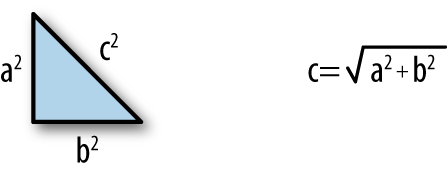
Figure 3-1. Pythagorean theorem
Triangle Inequality
One interesting aspect about the triangle in Figure 3-1 is that the length of the hypotenuse is always less than the length of each side added up individually (Figure 3-2).
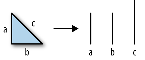
Figure 3-2. Triangle broken into three line segments
Stated mathematically: ∥x + y∥ ≤ ∥x∥ + ∥y∥. This inequality is important for finding a distance function; if the triangle inequality didn’t hold, what would happen is distances would become slightly distorted as you measure distance between points in a Euclidean space.
Geometrical Distance
The most intuitive distance functions are geometrical. Intuitively we can measure how far something is from one point to another. We already know about the Pythagorean theorem, but there are an infinite amount of possibilities that satisfy the triangle inequality.
Stated mathematically we can take the Pythagorean theorem and build what is called the Euclidean distance, which is denoted as:
As you can see, this is similar to the Pythagorean theorem, except it includes a sum. Mathematics gives us even greater ability to build distances by using something called a Minkowski distance (see Figure 3-3):
This p can be any integer and still satisfy the triangle inequality.
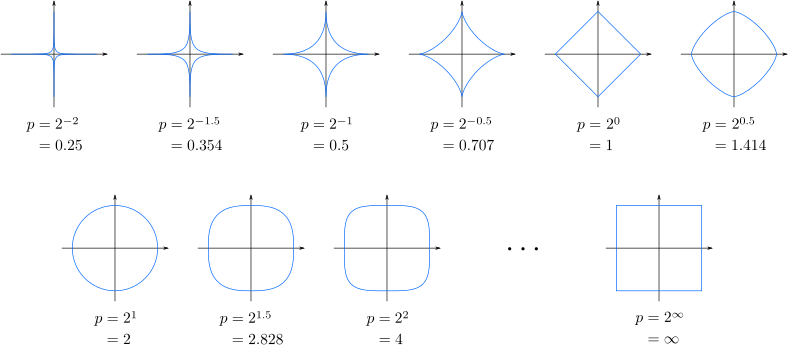
Figure 3-3. Minkowski distances as n increases (Source: Wikimedia)
Cosine similarity
One last geometrical distance is called cosine similarity or cosine distance. The beauty of this distance is its sheer speed at calculating distances between sparse vectors. For instance if we had 1,000 attributes collected about houses and 300 of these were mutually exclusive (meaning that one house had them but the others don’t), then we would only need to include 700 dimensions in the calculation.
Visually this measures the inner product space between two vectors and presents us with cosine as a measure. Its function is:
where ∥x∥ denotes the Euclidean distance discussed earlier.
Geometrical distances are generally what we want. When we talk about houses we want a geometrical distance. But there are other spaces that are just as valuable: computational, or discrete, as well as statistical distances.
Computational Distances
Imagine you want to measure how far it is from one part of the city to another. One way of doing this would be to utilize coordinates (longitude, latitude) and calculate a Euclidean distance. Let’s say you’re at Saint Edward State Park in Kenmore, WA (47.7329290, -122.2571466) and you want to meet someone at Vivace Espresso on Capitol Hill, Seattle, WA (47.6216650, -122.3213002).
Using the Euclidean distance we would calculate:
This is obviously a small result as it’s in degrees of latitude and longitude. To convert this into miles we would multiply it by 69.055, which yields approximately 8.9 miles (14.32 kilometers). Unfortunately this is way off! The actual distance is 14.2 miles (22.9 kilometers). Why are things so far off?
Note
Note that 69.055 is actually an approximation of latitude degrees to miles. Earth is an ellipsoid and therefore calculating distances actually depends on where you are in the world. But for such a short distance it’s good enough.
If I had the ability to lift off from Saint Edward State Park and fly to Vivace then, yes, it’d be shorter, but if I were to walk or drive I’d have to drive around Lake Washington (see Figure 3-4).
This gets us to the motivation behind computational distances. If you were to drive from Saint Edward State Park to Vivace then you’d have to follow the constraints of a road.
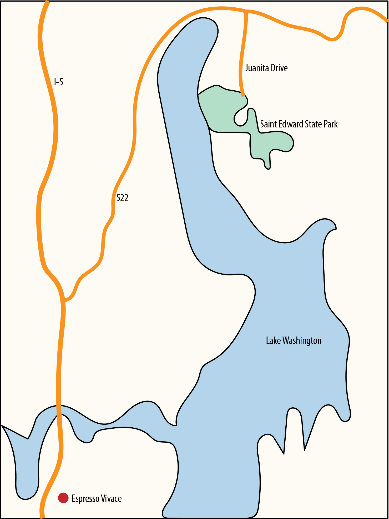
Figure 3-4. Driving to Vivace from Saint Edward State Park
Manhattan distance
This gets us into what is called the Taxicab distance or Manhattan distance.
Equation 3-2. Manhattan distance
Note that there is no ability to travel out of bounds. So imagine that your metric space is a grid of graphing paper and you are only allowed to draw along the boxes.
The Manhattan distance can be used for problems such as traversal of a graph and discrete optimization problems where you are constrained by edges. With our housing example, most likely you would want to measure the value of houses that are close by driving, not by flying. Otherwise you might include houses in your search that are across a barrier like a lake, or a mountain!
Levenshtein distance
Another distance that is commonly used in natural language processing is the Levenshtein distance. An analogy of how Levenshtein distance works is by changing one neighborhood to make an exact copy of another. The number of steps to make that happen is the distance. Usually this is applied with strings of characters to determine how many deletions, additions, or substitutions the strings require to be equal.
This can be quite useful for determining how similar neighborhoods are as well as strings. The formula for this is a bit more complicated as it is a recursive function, so instead of looking at the math we’ll just write Python for this:
deflev(a,b):ifnota:returnlen(b)ifnotb:returnlen(a)returnmin(lev(a[1:],b[1:])+(a[0]!=b[0]),lev(a[1:],b)+1,lev(a,b[1:])+1)
Statistical Distances
Last, there’s a third class of distances that I call statistical distances. In statistics we’re taught that to measure volatility or variance, we take pairs of datapoints and measure the squared difference. This gives us an idea of how dispersed the population is. This can actually be used when calculating distance as well, using what is called the Mahalanobis distance.
Imagine for a minute that you want to measure distance in an affluent neighborhood that is right on the water. People love living on the water and the closer you are to it, the higher the home value. But with our distances discussed earlier, whether computational or geometrical, we would have a bad approximation of this particular neighborhood because those distance calculations are primarily spherical in nature (Figures 3-5 and 3-6).
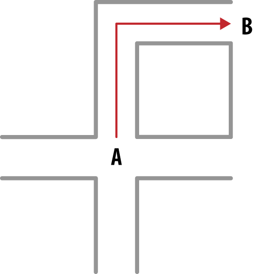
Figure 3-5. Driving from point A to point B on a city block
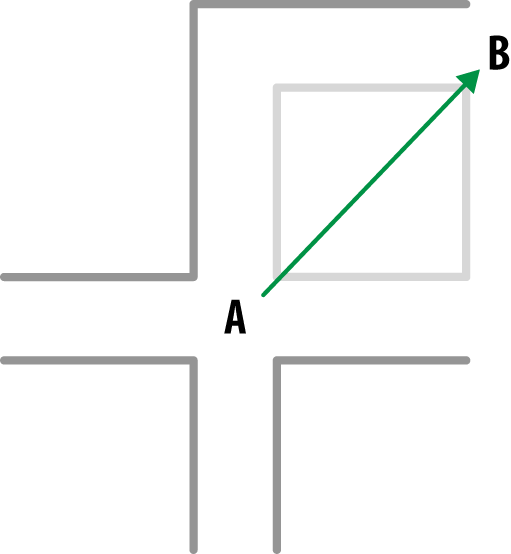
Figure 3-6. Straight line between A and B
This seems like a bad approach for this neighborhood because it is not spherical in nature. If we were to use Euclidean distances we’d be measuring values of houses not on the beach. If we were to use Manhattan distances we’d only look at houses close by the road.
Mahalanobis distance
Another approach is using the Mahalanobis distance. This takes into consideration some other statistical factors:
What this effectively does is give more stretch to the grouping of items (Figure 3-7):
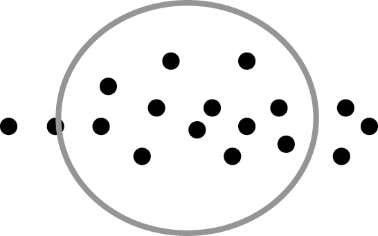
Figure 3-7. Mahalanobis distance
Jaccard distance
Yet another distance metric is called the Jaccard distance. This takes into consideration the population of overlap. For instance, if the number of attributes for one house match another, then they would be overlapping and therefore close in distance, whereas if the houses had diverging attributes they wouldn’t match. This is primarily used to quickly determine how similar text is by counting up the frequencies of letters in a string and then counting the characters that are not the same across both. Its formula is:
This finishes up a primer on distances. Now that we know how to measure what is close and what is far, how do we go about building a grouping or neighborhood? How many houses should be in the neighborhood?
Curse of Dimensionality
Before we continue, there’s a serious concern with using distances for anything and that is called the curse of dimensionality. When we model high-dimension spaces, our approximations of distance become less reliable. In practice it is important to realize that finding features of data sets is essential to making a resilient model. We will talk about feature engineering in Chapter 10 but for now be cognizant of the problem. Figure 3-8 shows a visual way of thinking about this.
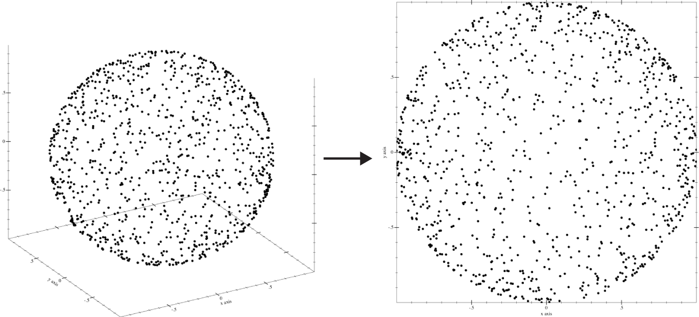
Figure 3-8. Curse of dimensionality
As Figure 3-8 shows, when we put random dots on a unit sphere and measure the distance from the origin (0,0,0), we find that the distance is always 1. But if we were to project that onto a 2D space, the distance would be less than or equal to 1. This same truth holds when we expand the dimensions. For instance, if we expanded our set from 3 dimensions to 4, it would be greater than or equal to 1. This inability to center in on a consistent distance is what breaks distance-based models, because all of the data points become chaotic and move away from one another.
How Do We Pick K?
Picking the number of houses to put into this model is a difficult problem—easy to verify but hard to calculate beforehand. At this point we know how we want to group things, but just don’t know how many items to put into our neighborhood. There are a few approaches to determining an optimal K, each with their own set of downsides:
-
Guessing
-
Using a heuristic
-
Optimizing using an algorithm
Guessing K
Guessing is always a good solution. Many times when we are approaching a problem, we have domain knowledge of it. Whether we are an expert or not, we know about the problem enough to know what a neighborhood is. My neighborhood where I live, for instance, is roughly 12 houses. If I wanted to expand I could set my K to 30 for a more flattened-out approximation.
Heuristics for Picking K
There are three heuristics that can help you determine an optimal K for a KNN algorithm:
-
Use coprime class and K combinations
-
Choose a K that is greater or equal to the number of classes plus one
-
Choose a K that is low enough to avoid noise
Use coprime class and K combinations
Picking coprime numbers of classes and K will ensure fewer ties. Coprime numbers are two numbers that don’t share any common divisors except for 1. So, for instance, 4 and 9 are coprime while 3 and 9 are not. Imagine you have two classes, good and bad. If we were to pick a K of 6, which is even, then we might end up having ties. Graphically it looks like Figure 3-9.
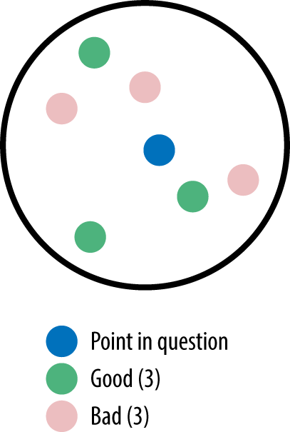
Figure 3-9. Tie with K=6 and two classes
If you picked a K of 5 instead (Figure 3-10), there wouldn’t be a tie.
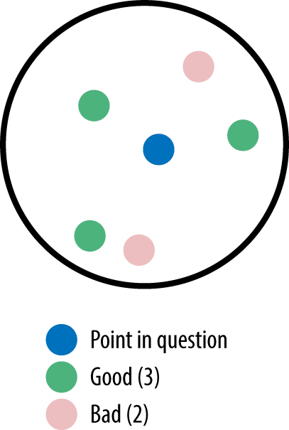
Figure 3-10. K=5 with two classes and no tie
Choose a K that is greater or equal to the number of classes plus one
Imagine there are three classes: lawful, chaotic, and neutral. A good heuristic is to pick a K of at least 3 because anything less will mean that there is no chance that each class will be represented. To illustrate, Figure 3-11 shows the case of K=2.
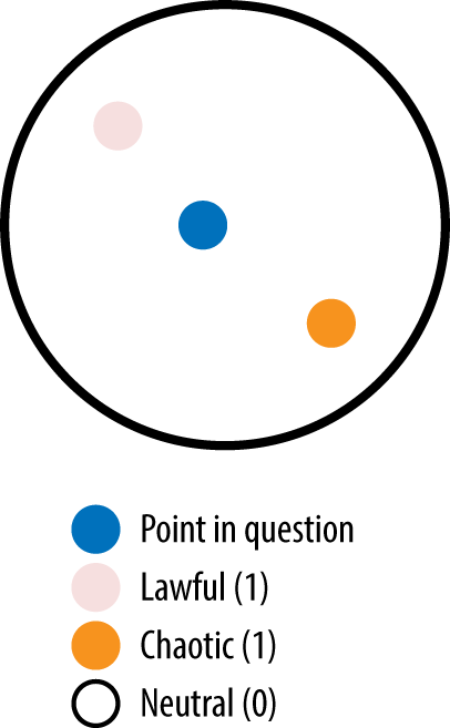
Figure 3-11. With K=2 there is no possibility that all three classes will be represented
Note how there are only two classes that get the chance to be used. Again, this is why we need to use at least K=3. But based on what we found in the first heuristic, ties are not a good thing. So, really, instead of K=3, we should use K=4 (as shown in Figure 3-12).
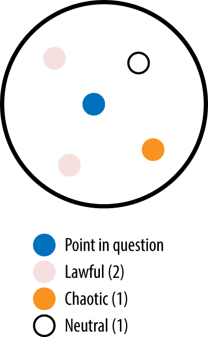
Figure 3-12. With K set greater than the number of classes, there is a chance for all classes to be represented
Choose a K that is low enough to avoid noise
As K increases, you eventually approach the size of the entire data set. If you were to pick the entire data set, you would select the most common class. A simple example is mapping a customer’s affinity to a brand. Say you have 100 orders as shown in Table 3-2.
| Brand | Count |
|---|---|
Widget Inc. |
30 |
Bozo Group |
23 |
Robots and Rockets |
12 |
Ion 5 |
35 |
Total |
100 |
If we were to set K=100, our answer will always be Ion 5 because Ion 5 is the distribution (the most common class) of the order history. That is not really what we want; instead, we want to determine the most recent order affinity. More specifically, we want to minimize the amount of noise that comes into our classification. Without coming up with a specific algorithm for this, we can justify K being set to a much lower rate, like K=3 or K=11.
Algorithms for picking K
Picking K can be somewhat qualitative and nonscientific, and that’s why there are many algorithms showing how to optimize K over a given training set. There are many approaches to choosing K, ranging from genetic algorithms to brute force to grid searches. Many people assert that you should determine K based on domain knowledge that you have as the implementor. For instance, if you know that 5 is good enough, you can pick that. This problem where you are trying to minimize error based on an arbitrary K is known as a hill climbing problem. The idea is to iterate through a couple of possible Ks until you find a suitable error. The difficult part about finding a K using an approach like genetic algorithms or brute force is that as K increases, the complexity of the classification also increases and slows down performance. In other words, as you increase K, the program actually gets slower. If you want to learn more about genetic algorithms applied to finding an optimal K, you can read more about it in Nigsch et al.’s Journal of Chemical Information and Modeling article, “Melting Point Prediction Employing k-Nearest Neighbor Algorithms and Genetic Parameter Optimization.” Personally, I think iterating twice through 1% of the population size is good enough. You should have a decent idea of what works and what doesn’t just by experimenting with different Ks.
Valuing Houses in Seattle
Valuing houses in Seattle is a tough gamble. According to Zillow, their Zestimate is consistently off in Seattle. Regardless, how would we go about building something that tells us how valuable the houses are in Seattle? This section will walk through a simple example so that you can figure out with reasonable accuracy what a house is worth based on freely available data from the King County Assessor.
If you’d like to follow along in the code examples, check out the GitHub repo.
About the Data
While the data is freely available, it wasn’t easy to put together. I did a bit of cajoling to get the data well formed. There’s a lot of features, ranging from inadequate parking to whether the house has a view of Mount Rainier or not. I felt that while that was an interesting exercise, it’s not really important to discuss here. In addition to the data they gave us, geolocation has been added to all of the datapoints so we can come up with a location distance much easier.
General Strategy
Our general strategy for finding the values of houses in Seattle is to come up with something we’re trying to minimize/maximize so we know how good the model is. Since we will be looking at house values explicitly, we can’t calculate an “Accuracy” rate because every value will be different. So instead we will utilize a different metric called mean absolute error.
With all models, our goal is to minimize or maximize something, and in this case we’re going to minimize the mean absolute error. This is defined as the average of the absolute errors. The reason we’ll use absolute error over any other common metrics (like mean squared error) is that it’s useful. When it comes to house values it’s hard to get intuition around the average squared error, but by using absolute error we can instead say that our model is off by $70,000 or similar on average.
As for unit testing and functional testing, we will approach this in a random fashion by stratifying the data into multiple chunks so that we can sample the mean absolute errors. This is mainly so that we don’t find just one weird case where the mean absolute error was exceptionally low. We will not be talking extensively here about unit testing because this is an early chapter and I feel that it’s more important to focus on the overall testing of the model through mean absolute error.
Coding and Testing Design
The basic design of the code for this chapter is going to center around a Regressor class. This class will take in King County housing data that comes in via a flat, calculate an error rate, and do the regression (Figure 3-13). We will not be doing any unit testing in this chapter but instead will visually test the code using the plot_error function we will build inside of the Regressor class.
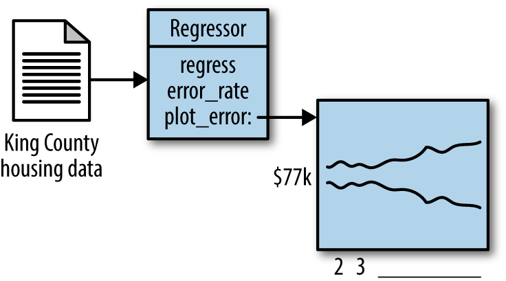
Figure 3-13. Overall coding design
For this chapter we will determine success by looking at the nuances of how our regressor works as we increase folds.
KNN Regressor Construction
To construct our KNN regression we will utilize something called a KDTree. It’s not essential that you know how these work but the idea is the KDTree will store data in a easily queriable fashion based on distance. The distance metric we will use is the Euclidean distance since it’s easy to compute and will suit us just fine. You could try many other metrics to see whether the error rate was better or worse.
importrandomimportsysimportpandasaspdimportnumpyasnpfromscipy.spatialimportKDTreefromsklearn.metricsimportmean_absolute_errorimportmatplotlib.pyplotaspltsys.setrecursionlimit(10000)classRegression(object):"""Performs kNN regression"""def__init__(self):self.k=5self.metric=np.meanself.kdtree=Noneself.houses=Noneself.values=Nonedefset_data(self,houses,values):"""Sets houses and values data:param houses: pandas.DataFrame with houses parameters:param values: pandas.Series with houses values"""self.houses=housesself.values=valuesself.kdtree=KDTree(self.houses)
Do note that we had to set the recursion limit higher since KDTree will recurse and throw an error otherwise.
There’s a few things we’re doing here I thought we should discuss. One of them is the idea of normalizing data. This is a great trick to make all of the data similar. Otherwise, what will happen is that we find something close that really shouldn’t be, or the bigger numbered dimensions will skew results.
On top of that we’re only selecting latitude and longitude and SqFtLot, because this is a proof of concept.
classRegression(object):# __init__# set_datadefregress(self,query_point):"""Calculates predicted value for house with particular parameters:param query_point: pandas.Series with house parameters:return: house value"""_,indexes=self.kdtree.query(query_point,self.k)value=self.metric(self.values.iloc[indexes])ifnp.isnan(value):raiseException('Unexpected result')else:returnvalue
Here we are querying the KDTree to find the closest K houses. We then use the metric, in this case mean, to calculate a regression value.
At this point we need to focus on the fact that, although all of this is great, we need some sort of test to make sure our data is working properly.
KNN Testing
Up until this point we’ve written a perfectly reasonable KNN regression tool to tell us house prices in King County. But how well does it actually perform? To do that we use something called cross-validation, which involves the following generalized algorithm:
-
Take a training set and split it into two categories: testing and training
-
Use the training data to train the model
-
Use the testing data to test how well the model performs.
We can do that with the following code:
classRegressionTest(object):"""Take in King County housing data, calculate andplot the kNN regression error rate."""def__init__(self):self.houses=Noneself.values=Nonedefload_csv_file(self,csv_file,limit=None):"""Loads CSV file with houses data:param csv_file: CSV file name:param limit: number of rows of file to read"""houses=pd.read_csv(csv_file,nrows=limit)self.values=houses['AppraisedValue']houses=houses.drop('AppraisedValue',1)houses=(houses-houses.mean())/(houses.max()-houses.min())self.houses=housesself.houses=self.houses[['lat','long','SqFtLot']]deftests(self,folds):"""Calculates mean absolute errors for series of tests:param folds: how many times split the data:return: list of error values"""holdout=1/float(folds)errors=[]for_inrange(folds):values_regress,values_actual=self.test_regression(holdout)errors.append(mean_absolute_error(values_actual,values_regress))returnerrorsdeftest_regression(self,holdout):"""Calculates regression for out-of-sample data:param holdout: part of the data for testing [0,1]:return: tuple(y_regression, values_actual)"""test_rows=random.sample(self.houses.index.tolist(),int(round(len(self.houses)*holdout)))train_rows=set(range(len(self.houses)))-set(test_rows)df_test=self.houses.ix[test_rows]df_train=self.houses.drop(test_rows)train_values=self.values.ix[train_rows]regression=Regression()regression.set_data(houses=df_train,values=train_values)values_regr=[]values_actual=[]foridx,rowindf_test.iterrows():values_regr.append(regression.regress(row))values_actual.append(self.values[idx])returnvalues_regr,values_actual
Folds are generally how many times you wish to split the data. So for instance if we had 3 folds we would hold 2/3 of the data for training and 1/3 for testing and iterate through the problem set 3 times (Figure 3-14).
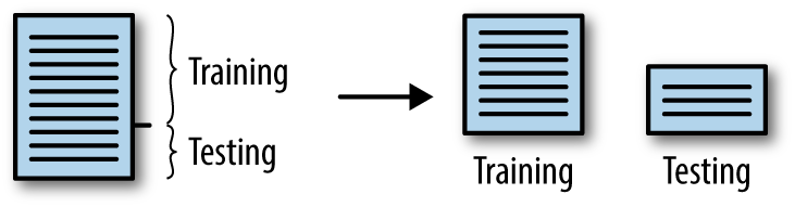
Figure 3-14. Split data into training and testing
Now these datapoints are interesting, but how well does our model perform? To do that, let’s take a visual approach and write code that utilizes Pandas’ graphics and matplotlib.
classRegressionTest(object):# __init__# load_csv_file# tests# test_regressiondefplot_error_rates(self):"""Plots MAE vs #folds"""folds_range=range(2,11)errors_df=pd.DataFrame({'max':0,'min':0},index=folds_range)forfoldsinfolds_range:errors=self.tests(folds)errors_df['max'][folds]=max(errors)errors_df['min'][folds]=min(errors)errors_df.plot(title='Mean Absolute Error of KNN over different folds_range')plt.xlabel('#folds_range')plt.ylabel('MAE')plt.show()
We finally run this by running the following script:
defmain():regression_test=RegressionTest()regression_test.load_csv_file('king_county_data_geocoded.csv',100)regression_test.plot_error_rates()if__name__=='__main__':main()
Running this yields the graph in Figure 3-15.
As you can see, starting with folds of 2 we have a fairly tight absolute deviation of about $77,000 dollars. As we increase the folds and, as a result, reduce the testing sample, that increases to a range of $73,000 to $77,000. For a very simplistic model that contains all information from waterfront property to condos, this actually does quite well!
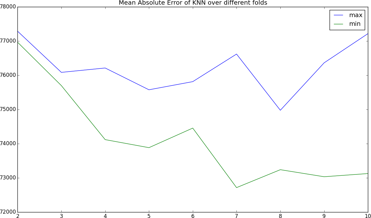
Figure 3-15. The error rates we achieved. The x-axis is the number of folds, and the y-axis is the absolute error in estimated home price (i.e., how much it’s off by).
Conclusion
While K-Nearest Neighbors is a simple algorithm, it yields quite good results. We have seen that for distance-based problems we can utilize KNN to great effect. We also learned about how you can use this algorithm for either a classification or regression problem. We then analyzed the regression we built using a graphic representing the error.
Next, we showed that KNN has a downside that is inherent in any distance-based metric: the curse of dimensionality. This curse is something we can overcome using feature transformations or selections.
Overall it’s a great algorithm and it stands the test of time.
1 Van Ommeren et al., “Estimating the Marginal Willingness to Pay for Commuting,” Journal of Regional Science 40 (2000): 541–63.