Fitness of a Cluster

Domain knowledge can become very useful in determining the fitness of an unsupervised model. For instance, if we want to find things that are similar, we might use some sort of distance-based metric. If instead we wish to determine independent factors of the data, we might calculate fitness based on correlation or covariance.

Possible fitness functions include:

• Mean distance from centroid

• Mean distance from all points in a cluster

• Silhouette coefficient

Mean distances from centroid, or from all points in a cluster, are almost baked into algorithms that we will be talking about such as K-Means or EM clustering, but the silhouette coefficient is an interesting take on fitness of cluster mappings.

Silhouette Coefficient

The silhouette coefficient evaluates cluster performance without ground truth (i.e., data that has been provided through direct observation versus inferred observations) by looking at the relation of the average distance inside of a cluster versus the average distance to the nearest cluster (Figure 9-1).

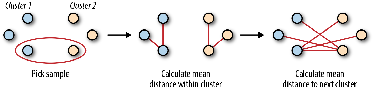
Figure 9-1. Silhouette coefficient visually

Mathematically the metric is:

where a is the average distance between a sample and all other points in that cluster and b is the same sample’s mean distance to the next nearest cluster points.

This coefficient ends up becoming useful because it will show fitness on a scale of –1 to 1 while not requiring ground truth.

Comparing Results to Ground Truth

In practice many times machine learning involves utilizing ground truth, which is something that we can usually find through trained data sets, humans, or other means like test equipment. This data is valuable in testing our intuition and determining how fitting our model is.

Clustering can be tested using ground truth using the following means:

• Rand index

• Mutual information

• Homogeneity

• Completeness

• V-measure

• Fowlkes-Mallows score

All of these methods can be extremely useful in determining how fit a model is. scikit-learn implements all of these and can easily be used to determine a score.

The K-Means Algorithm

The K-Means algorithm starts with a base case. Pick K random points in the data set and define them as centroids. Next, assign each point to a cluster number that is closest to each different centroid. Now we have a clustering based on the original randomized centroid. This is not exactly what we want to end with, so we update where the centroids are using a mean of the data. At that point we repeat until the centroids no longer move (Figure 9-2).

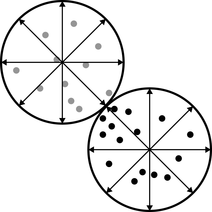
Figure 9-2. In a lot of ways, K-Means resembles a pizza

To construct K-Means clusters we need to have some sort of measurement for distance from the center. Back in Chapter 3 we introduced a few distance metrics, such as:

Manhattan distance

$d_{manhattan}(x,y)={\sum }_{i=1}^n|x_i-y_i|$

Euclidean distance

$d_{euclid}(x,y)=\sqrt{{\sum }_{i=1}^n{(x_i-y_i)}^2}$

Minkowski distance

$d(x,y)={({\sum }_{i=1}^n\mid x_i-y_i{\mid }^p)}^{\frac{1}{p}}$

Mahalanobis distance

$d(x,y)=\sqrt{{\sum }_{i=1}^n\frac{{(x_i-y_i)}^2}{s_i^2}}$

For a refresher on the metrics discussed here, review K-Nearest Neighbors in Chapter 3.

Downside of K-Means Clustering

One drawback of this procedure is that everything must have a hard boundary. This means that a data point can only be in one cluster and not straddle the line between two of them. K-Means also prefers spherical data since most of the time the Euclidean distance is being used. When looking at a graphic like Figure 9-3, where the data in the middle could go either direction (to a cluster on the left or right), the downsides become obvious.

Algorithm

The EM clustering algorithm is an iterative process to converge on a cluster mapping. It completes two steps in each iteration: expect and maximize.

But what does that mean? Expectation and maximization could mean a lot.

Setup Notes

All of the code we’re using for this example can be found on GitHub.

Python is constantly changing so the README is the best place to come up to speed on running the examples.

Gathering the Data

There is a massive amount of data on music from the 1100s through today. We have MP3s, CDs, vinyl records, and written music. Without trying to classify the entire world of music, let’s determine a small subsection that we can use. Since I don’t want to engage in any copyright suits we will only use public information on albums. This would be Artist, Song Name, Genre (if available), and any other characteristics we can find. To achieve this we have access to a plethora of information contained in Discogs.com. They offer many XML data dumps of records and songs.

Also, since we’re not trying to cluster the entire data set of albums in the world, let’s just focus on jazz. Most people would agree that jazz is a genre that is hard to really classify into any category. It could be fusion, or it could be steel drums.

To get our data set I downloaded metadata (year, artist, genre, etc.) for the best jazz albums (according to http://www.scaruffi.com/jazz/best100.html). The data goes back to 1940 and well into the 2000s. In total I was able to download metadata for about 1,200 unique records. All great albums!

But that isn’t enough information. On top of that I annotated the information by using the Discogs API to determine the style of jazz music in each.

After annotating the original data set I found that there are 128 unique styles associated with jazz (at least according to Discogs). They range from aboriginal to vocal.

Coding Design

Although this chapter uses two different algorithms (EM clustering and K-Means clustering), the code will focus on EM clustering and will follow the data flow in Figure 9-4.

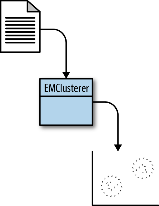
Figure 9-4. EM clustering class

Analyzing the Data with K-Means

Like we did with KNN, we need to figure out an optimal K. Unfortunately with clustering there really isn’t much we can test with except to just see whether we split into two different clusters.

But let’s say that we want to fit all of our records on a shelf and have 25 slots—similar to the IKEA bookshelf. We could run a clustering of all of our data using K = 25.

import csv

from sklearn.cluster import KMeans

data = []
artists = []
years = []
with open('data/annotated_jazz_albums.csv', 'r') as csvfile:
  reader = csv.DictReader(csvfile)
  headers = reader.fieldnames[3:]
  for row in reader:
    artists.append(row['artist_album'])
    years.append(row['year'])
    data.append([int(row[key]) for key in headers])

clusters = KMeans(n_clusters=25).fit_predict(data)

with open('data/clustered_kmeans.csv', 'w') as csvfile:
  fieldnames = ['artist_album', 'year', 'cluster']
  writer = csv.DictWriter(csvfile, fieldnames=fieldnames)

  writer.writeheader()

  for i, cluster in enumerate(clusters):
    writer.writerow({'artist_album': artists[i],
             'year': years[i],
             'cluster': cluster})

That’s it! Of course clustering without looking at what this actually tells us is useless. This does split the data into 25 different categories, but what does it all mean?

Looking at a graphic of year versus assigned cluster number yields interesting results (Figure 9-5).

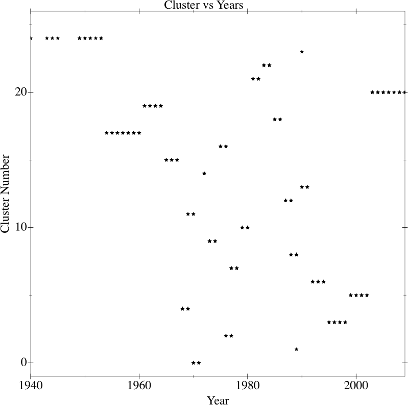
Figure 9-5. K-Means applied to jazz albums

As you can see, jazz starts out in the Big Band era pretty much in the same cluster, transitions into cool jazz, and then around 1959 it starts to go everywhere until about 1990 when things cool down a bit. What’s fascinating is how well that syncs up with jazz history.

What happens when we cluster the data using EM clustering?

EM Clustering Our Data

With EM clustering, remember that we are probabilistically assigning to different clusters—it isn’t 100% one or the other. This could be highly useful for our purposes since jazz has so much crossover.

Let’s go through the process of writing our own code and then use it to map the same data that we have from our jazz data set, then see what happens.

Our first step is to be able to initialize the cluster. If you remember we need to have indicator variables z_t that follow a uniform distribution. These tell us the probability that each data point is in each cluster.

Stepping back into our example, we first need to write a helper function that returns the density of a multivariate normal distribution. This is based on how R does this:

from collections import namedtuple
import random
import logging
import math

import numpy as np
from numpy.linalg import LinAlgError

def dvmnorm(x, mean, covariance, log=False):
  """density function for the multivariate normal distribution
  based on sources of R library 'mvtnorm'
  :rtype : np.array
  :param x: vector or matrix of quantiles. If x is a matrix, each row is taken
  to be a quantile
  :param mean: mean vector, np.array
  :param covariance: covariance matrix, np.array
  :param log: if True, densities d are given as log(d), default is False
  """
  n = covariance.shape[0]
  try:
    dec = np.linalg.cholesky(covariance)
  except LinAlgError:
    dec = np.linalg.cholesky(covariance + np.eye(covariance.shape[0]) * 0.0001)
  tmp = np.linalg.solve(dec, np.transpose(x - mean))
  rss = np.sum(tmp * tmp, axis=0)
  logretval = -np.sum(np.log(np.diag(dec))) - 
              0.5 * n * np.log(2 * math.pi) - 0.5 * rss
  if log:
    return logretval
  else:
    return np.exp(logretval)

Using all this setup we can now build an EMClustering class that will do our EM clustering and log outputs as needed.

This class has the following methods of note:

partitions

Will return the cluster mappings of the data if they are set.

data

Will return the data object passed in.

labels

Will return the membership weights for each cluster.

clusters

Will return the clusters.

setup

This does all of the setup for the EM clustering.

class EMClustering(object):
  logger = logging.getLogger(__name__)
  ch = logging.StreamHandler()
  formatstring = '%(asctime)s - %(name)s - %(levelname)s - %(message)s'
  formatter = logging.Formatter(formatstring)
  ch.setFormatter(formatter)
  logger.addHandler(ch)
  logger.setLevel(logging.DEBUG)

  cluster = namedtuple('cluster', 'weight, mean, covariance')

  def __init__(self, n_clusters):
    self._data = None
    self._clusters = None
    self._membership_weights = None
    self._partitions = None
    self._n_clusters = n_clusters

  @property
  def partitions(self):
    return self._partitions

  @property
  def data(self):
    return self._data

  @property
  def labels(self):
    return self._membership_weights

  @property
  def clusters(self):
    return self._clusters

  def setup(self, data):
    self._n_samples, self._n_features = data.shape
    self._data = data
    self._membership_weights = np.ones((self._n_samples, self._n_clusters)) / 
                               self._n_clusters
    self._s = 0.2

    indices = list(range(data.shape[0]))
    random.shuffle(indices)
    pick_k_random_indices = random.sample(indices, self._n_clusters)

    self._clusters = []
    for cluster_num in range(self._n_clusters):
      mean = data[pick_k_random_indices[cluster_num], :]
      covariance = self._s * np.eye(self._n_features)
      mapping = self.cluster(1.0 / self._n_clusters, mean, covariance)
      self._clusters.append(mapping)

    self._partitions = np.empty(self._n_samples, dtype=np.int32)

At this point we have set up all of our base case stuff. We have @k, which is the number of clusters, @data is the data we pass in that we want to cluster, @labels are an array full of the probabilities that the row is in each cluster, and @classes holds on to an array of means and covariances, which tells us where the distribution of data is. Last, @partitions are the assignments of each data row to cluster index.

Now we need to build our expectation step, which is to figure out what the probability of each data row is in each cluster. To do this we need to write a new method, expect, which will do this:

class EMClustering(object):
  # __init__
  # setup()

  def expect(self):
    log_likelyhood = 0
    for cluster_num, cluster in enumerate(self._clusters):
      log_density = dvmnorm(self._data, cluster.mean, 
                            cluster.covariance, log=True)
      membership_weights = cluster.weight * np.exp(log_density)
      log_likelyhood += sum(log_density * 
                            self._membership_weights[:, cluster_num])

      self._membership_weights[:, cluster_num] = membership_weights

    for sample_num, probabilities in enumerate(self._membership_weights):
      prob_sum = sum(probabilities)

      self._partitions[sample_num] = np.argmax(probabilities)

      if prob_sum == 0:
        self._membership_weights[sample_num, :] = np.ones_like(probabilities) / 
                                                  self._n_clusters
      else:
        self._membership_weights[sample_num, :] = probabilities / prob_sum

    self.logger.debug('log likelyhood %f', log_likelyhood)

The first part of this code iterates through all classes, which holds on to the means and covariances of each cluster. From there we want to find the inverse covariance matrix and the determinant of the covariance. For each row we calculate a value that is proportional to the probability that the row is in a cluster. This is:

This is effectively a Gaussian distance metric to help us determine how far outside of the mean our data is.

Let’s say that the row vector is exactly the mean. This equation would reduce down to p_ij = det(C), which is just the determinant of the covariance matrix. This is actually the highest value you can get out of this function. If for instance the row vector was far away from the mean vector, then p_ij would become smaller and smaller due to the exponentiation and negative fraction in the front.

The nice thing is that this is proportional to the Gaussian probability that the row vector is in the mean. Since this is proportional and not equal to, in the last part we end up normalizing to sum up to 1.

Now we can move on to the maximization step:

class EMClustering(object):
  # __init__
  # setup()
  # expect

  def maximize(self):
    for cluster_num, cluster in enumerate(self._clusters):
      weights = self._membership_weights[:, cluster_num]
      weight = np.average(weights)
      mean = np.average(self._data, axis=0, weights=weights)
      covariance = np.cov(self._data, rowvar=False, ddof=0, aweights=weights)
      self._clusters[cluster_num] = self.cluster(weight, mean, covariance)

Again here we are iterating over the clusters called @classes. We first make an array called sum that holds on to the weighted sum of the data happening. From there we normalize to build a weighted mean. To calculate the covariance matrix we start with a zero matrix that is square and the width of our clusters. Then we iterate through all row vectors and incrementally add on the weighted difference of the row and the mean for each combination of the matrix. Again at this point we normalize and store.

Now we can get down to using this. To do that we add two convenience methods that help in querying the data:

class EMClustering(object):
  # __init__
  # setup
  # expect
  # maximize

  def fit_predict(self, data, iteration=5):
    self.setup(data)
    for i in range(iteration):
      self.logger.debug('Iteration %d', i)
      self.expect()
      self.maximize()
    return self

The Results from the EM Jazz Clustering

Back to our results of EM clustering with our jazz music. To actually run the analysis we run the following script:

import csv

import numpy as np

from em_clustering import EMClustering

np.set_printoptions(threshold=9000)

data = []
artists = []
years = []

# with open('data/less_covariance_jazz_albums.csv', 'rb') as csvfile:
with open('data/annotated_jazz_albums.csv', 'r') as csvfile:
  reader = csv.DictReader(csvfile)
  headers = reader.fieldnames[3:]
  for row in reader:
    artists.append(row['artist_album'])
    years.append(row['year'])
    data.append([int(row[key]) for key in headers])

clusterer = EMClustering(n_clusters=25)
clusters = clusterer.fit_predict(np.array(data))

print(clusters.partitions)

The first thing you’ll notice about EM clustering is that it’s slow. It’s not as quick as calculating new centroids and iterating. It has to calculate covariances and means, which are all inefficient. Ockham’s Razor would tell us here that EM clustering is most likely not a good use for clustering big amounts of data.

The other thing that you’ll notice is that our annotated jazz music will not work because the covariance matrix of this is singular. This is not a good thing; as a matter of fact this problem is ill suited for EM clustering because of this, so we have to transform it into a different problem altogether.

We do that by collapsing the dimensions into the top two genres by index:

import csv

with open('data/less_covariance_jazz_albums.csv', 'w') as csvout:
  writer = csv.writer(csvout, delimiter=',')

  # Write the header of the CSV file
  writer.writerow(['artist_album', 'key_index', 'year', 'Genre_1', 'Genre_2'])

  with open('data/annotated_jazz_albums.csv', 'r') as csvin:
    reader = csv.DictReader(csvin)
    for row in reader:
      genre_count = 0
      genres = [0, 0]
      genre_idx = 0
      idx = 0
      for key, value in row.items():
        break if genre_idx == 2
        if value == '1':
          genres[genre_idx] = idx
          genre_idx += 1
        idx += 1
      if genres[0] > 0 || genres[1] > 0:
        line = [row['artist_album'], row['key_index'], 
                row['year'], genres[0], genres[1]]
        writer.writerow(line)

Basically what we are doing here is saying for the first two genres, let’s assign a genre index to it and store it. We’ll skip any albums with zero information assigned to them.

At this point we are able to run the EM clustering algorithm, except that things become too difficult to actually cluster. This is an important lesson with EM clustering. The data we have actually doesn’t cluster because the matrix has become too unstable to invert.

Some possibilities for refinement would be to try out K-Means or other clustering algorithms, but really a better approach would be to work on the data some more. Jazz albums are a fun example but data-wise aren’t very illustrative. We could, for instance, expand using some more musical genomes, or feed this into some sort of text-based model. Or maybe we could spelunk for musical queues using fast Fourier transforms! The possibilities are really endless but this gives us a good start.