Streaming Architecture

Because there are so many streaming systems and ways of doing streaming, and because everything is evolving quickly, we have to narrow our focus to a representative sample of current systems and a reference architecture that covers the essential features.

Figure 2-1 shows this fast data architecture.

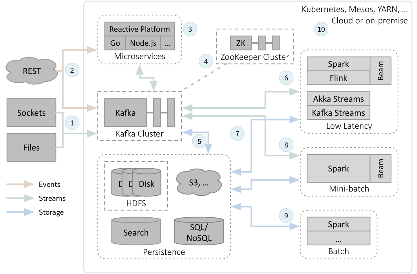
Figure 2-1. Fast data (streaming) architecture

There are more parts in Figure 2-1 than in Figure 1-1, so I’ve numbered elements of the figure to aid in the discussion that follows. Mini-clusters for Kafka, ZooKeeper, and HDFS are indicated by dashed rectangles. General functional areas, such as persistence and low-latency streaming engines, are indicated by the dotted, rounded rectangles.

Let’s walk through the architecture. Subsequent sections will explore the details:

1. Streams of data arrive into the system from several possible sources. Sometimes data is read from files, like logs, and other times data arrives over sockets from servers within the environment or from external sources, such as telemetry feeds from IoT devices in the field, or social network feeds like the Twitter “firehose.” These streams are typically records, which don’t require individual handling like events that trigger state changes. They are ingested into a distributed Kafka cluster for scalable, durable, reliable, but usually temporary, storage. The data is organized into topics, which support multiple producers and consumers per topic and some ordering guarantees. Kafka is the backbone of the architecture. The Kafka cluster may use dedicated servers, which provides maximum load scalability and minimizes the risk of compromised performance due to “noisy neighbor” services misbehaving on the same machines. On the other hand, strategic colocation of some other services can eliminate network overhead. In fact, this is how Kafka Streams works, as a library on top of Kafka (see also number 6).

2. REST (Representational State Transfer) requests are often synchronous, meaning a completed response is expected “now,” but they can also be asynchronous, where a minimal acknowledgment is returned now and the completed response is returned later, using WebSockets or another mechanism. Normally REST is used for sending events to trigger state changes during sessions between clients and servers, in contrast to records of data. The overhead of REST means it is less ideal as a data ingestion channel for high-bandwidth data flows. Still, REST for data ingestion into Kafka is still possible using custom microservices or through Kafka Connect’s REST interface.

3. A real environment will need a family of microservices for management and monitoring tasks, where REST is often used. They can be implemented with a wide variety of tools. Shown here are the Lightbend Reactive Platform (RP), which includes Akka, Play, Lagom, and other tools, and the Go and Node.js ecosystems, as examples of popular, modern tools for implementing custom microservices. They might stream state updates to and from Kafka, which is also a good way to integrate our time-sensitive analytics with the rest of our microservices. Hence, our architecture needs to handle a wide range of application types and characteristics.

4. Kafka is a distributed system and it uses ZooKeeper (ZK) for tasks requiring consensus, such as leader election and storage of some state information. Other components in the environment might also use ZooKeeper for similar purposes. ZooKeeper is deployed as a cluster, often with its own dedicated hardware, for the same reasons that Kafka is often deployed this way.

5. With Kafka Connect, raw data can be persisted from Kafka to longer-term, persistent storage. The arrow is two-way because data from long-term storage can also be ingested into Kafka to provide a uniform way to feed downstream analytics with data. When choosing between a database or a filesystem, keep in mind that a database is best when row-level access (e.g., CRUD operations) is required. NoSQL provides more flexible storage and query options, consistency versus availability (CAP) trade-offs, generally better scalability, and often lower operating costs, while SQL databases provide richer query semantics, especially for data warehousing scenarios, and stronger consistency. A distributed filesystem, such as HDFS, or object store, such as AWS S3, offers lower cost per gigabyte storage compared to databases and more flexibility for data formats, but is best used when scans are the dominant access pattern, rather than per-record CRUD operations. A search appliance, like Elasticsearch, is often used to index data for fast queries.

6. For low-latency stream processing, the most robust mechanism is to ingest data from Kafka into the stream processing engine. There are quite a few engines currently vying for attention, and I’ll discuss four widely used engines that cover a spectrum of needs.¹

   You can evaluate other alternatives using the concepts we’ll discuss in this report. Apache Spark’s Structured Streaming and Apache Flink are grouped together because they run as distributed services to which you submit jobs to run. They provide similar, very rich analytics, inspired in part by Apache Beam, which has been a leader in defining advanced streaming semantics. In fact, both Spark and Flink can function as “runners” for data flows defined with Beam. Akka Streams and Kafka Streams are grouped together because they run as libraries that you embed in your microservices, providing greater flexibility in how you integrate analytics with other processing, with very low latency and lower overhead than Spark and Flink. Kafka Streams also offers a SQL query service, while Akka Streams integrates with the rich Akka ecosystem of microservice tools. Neither is designed to be as full-featured as Beam-compatible systems. All these tools support distribution in one way or another across a cluster (not shown), usually in collaboration with the underlying clustering system (e.g., Kubernetes, Mesos, or YARN; see number 10). It’s unlikely you would need or want all four streaming engines. Results from any of these tools can be written back to new Kafka topics for downstream consumption. While it’s possible to read and write data directly between other sources and these tools, the durability and reliability of Kafka ingestion and the benefits of having one access method make it an excellent default choice despite the modest extra overhead of going through Kafka. For example, if a process fails, the data can be reread from Kafka by a restarted process. It is often not an option to requery an incoming data source directly.

7. Stream processing results can also be written to persistent storage and data can be ingested from storage. This is useful when O(1) access for particular records is desirable, rather than O(N) to scan a Kafka topic. It’s also more suitable for longer-term storage than storing in a Kafka topic. Reading from storage enables analytics that combine long-term historical data and streaming data.

8. The mini-batch model of Spark, called Spark Streaming, is the original way that Spark supported streaming, where data is captured in fixed time intervals, then processed as a “mini batch.” The drawback is longer latencies are required (100 milliseconds or longer for the intervals), but when low latency isn’t required, the extra window of time is valuable for more expensive calculations, such as training machine learning models using Spark’s MLlib or other libraries. As before, data can be moved to and from Kafka. However, Spark Streaming is becoming obsolete now that Structured Streaming is mature, so consider using the latter instead.

9. Since you have Spark and a persistent store, like HDFS or a database, you can still do batch-mode processing and interactive analytics. Hence, the architecture is flexible enough to support traditional analysis scenarios too. Batch jobs are less likely to use Kafka as a source or sink for data, so this pathway is not shown.

10. All of the above can be deployed in cloud environments like AWS, Google Cloud Environment, and Microsoft Azure, as well as on-premise. Cluster resources and job management can be managed by Kubernetes, Mesos, and Hadoop/YARN. YARN is most mature, but Kubernetes and Mesos offer much greater flexibility for the heterogeneous nature of this architecture.

When I discussed Hadoop, I mentioned that the three essential components are HDFS for storage, MapReduce and Spark for compute, and YARN for the control plane. In the fast data architecture for streaming applications, the analogs are the following:

• Storage: Kafka

• Compute: Spark, Flink, Akka Streams, and Kafka Streams

• Control plane: Kerberos and Mesos, or YARN with limitations

Let’s see where the sweet spots are for streaming jobs compared to batch jobs (Table 2-1).

While the fast data architecture can store the same petabyte data sets, a streaming job will typically operate on megabyte to terabyte at any one time. A terabyte per minute, for example, would be a huge volume of data! The low-latency engines in Figure 2-1 operate at subsecond latencies, in some cases down to microseconds.

However, you’ll notice that the essential components of a big data architecture like Hadoop are also present, such as Spark and HDFS. In large clusters, you can run your new streaming workloads and microservices, along with the batch and interactive workloads for which Hadoop is well suited. They are still supported in the fast data architecture, although the wealth of third-party add-ons in the Hadoop ecosystem isn’t yet matched in the newer Kubernetes and Mesos communities.

What About the Lambda Architecture?

In 2011, Nathan Marz introduced the lambda architecture, a hybrid model that uses three layers:

• A batch layer for large-scale analytics over historical data

• A speed layer for low-latency processing of newly arrived data (often with approximate results)

• A serving layer to provide a query/view capability that unifies the results of the batch and speed layers.

The fast data architecture can be used to implement applications following the lambda architecture pattern, but this pattern has drawbacks.²

First, without a tool like Spark that can be used to implement logic that runs in both batch and streaming jobs, you find yourself implementing logic twice: once using the tools for the batch layer and again using the tools for the speed layer. The serving layer typically requires custom tools as well, to integrate the two sources of data. However, if everything is considered a “stream”—either finite, as in batch processing, or unbounded—then batch processing becomes just a subset of stream processing, requiring only a single implementation.

Second, the lambda architecture emerged before we understood how to perform the same accurate calculations in a streaming context that we were accustomed to doing in a batch context. The assumption was that streaming calculations could only be approximate, meaning that batch calculations would always be required for definitive results. That’s changed, as we’ll explore in Chapter 4.

In retrospect, the lambda architecture is an important transitional step toward the fast data architecture, although it can still be a useful pattern in some situations.

Now that we’ve completed our high-level overview, let’s explore the core principles required for the fast data architecture, beginning with the need for a data backplane.