Chapter 3. Dictionaries and Sets
May your hashes be unique,
Your keys rarely collide,
And your dictionaries
be forever ordered.1Brandon Rhodes, in The Dictionary Even Mightier
The dict type is not only widely used in our programs but also a fundamental part of the Python implementation. Class and instance attributes, module namespaces, and function keyword arguments are some of the fundamental Python constructs represented by dictionaries in memory. The built-in functions are all in __builtins__.__dict__.
Because of their crucial role, Python dicts are highly optimized—and continue to get improvements. Hash tables are the engines behind Python’s high-performance dicts.
Other built-in types based on hash tables are set and frozenset. These offer richer APIs and operators than the sets you may have encountered in other popular languages. In particular, Python sets implement all the fundamental operations from set theory, like union, intersection, subset tests etc. With them, we can express algorithms in a more declarative way, avoiding lots of nested loops and conditionals.
Here is a brief outline of this chapter:
-
Common dictionary methods
-
Special handling for missing keys
-
Variations of
dictin the standard library -
The
setandfrozensettypes -
How hash tables work
-
Implications of hash tables in the behavior of sets and dictionaries.
What’s new in this chapter
The dict implementation evolved from what I described in 1st edition of Fluent Python. Major revisions in this chapter are:
-
Explanation of the hash table algorithm now starts with its use in
set, which is simpler to understand. -
Coverage of the memory optimizations that preserve key insertion order in
dictinstances—implemented in Python 3.6—and the key-sharing layout for dictionaries holding instance attributes—the__dict__of used-defined objects since Python 3.3. -
New section on the view objects returned by
dict.keys,dict.items, anddict.valuessince Python 3.0.
Note
One minor change: I adopted the term hash code instead of hash value, because we need to talk about object values to understand hashing, and it is easier to keep the two concepts apart in a sentence like this: “The hash code is derived from the object value.” However, I keep the original term when I quote the Python documentation.
Standard API of Mapping Types
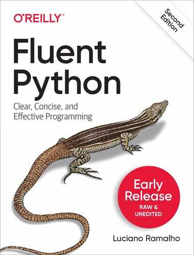
The collections.abc module provides the Mapping and MutableMapping ABCs describing the interfaces of dict and similar types. See Figure 3-1.
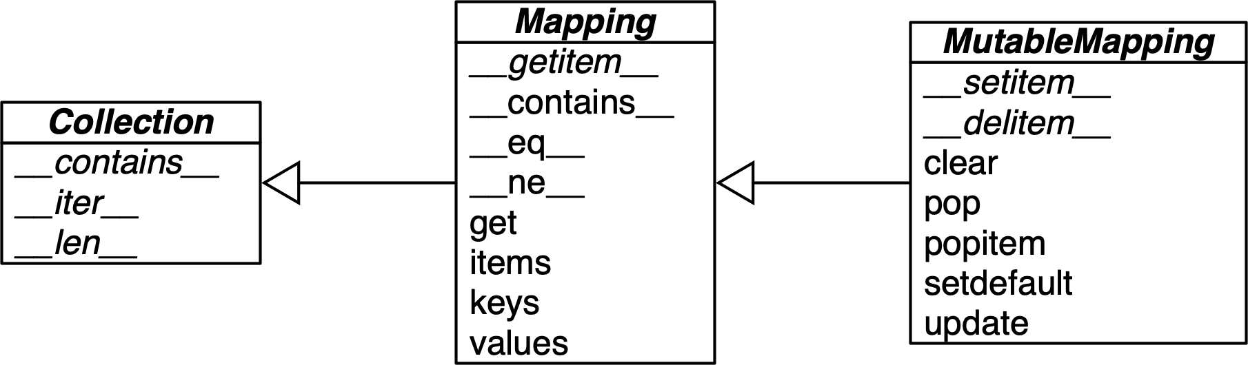
Figure 3-1. Simplified UML class diagram for the MutableMapping and its superclasses from collections.abc (inheritance arrows point from subclasses to superclasses; names in italic are abstract classes and abstract methods)
The main value of the ABCs is documenting and formalizing the standard interfaces for mappings, and serving as criteria for isinstance tests in code that needs to support mappings in a broad sense:
>>>my_dict={}>>>isinstance(my_dict,abc.Mapping)True>>>isinstance(my_dict,abc.MutableMapping)True
Tip
Using isinstance with an ABC is often better than checking whether a function argument is of the concrete dict type, because then alternative mapping types can be used. We’ll discuss this in detail in [Link to Come].
To implement a custom mapping, it’s easier to extend collections.UserDict, or to wrap a dict by composition, instead of subclassing these ABCs. The collections.UserDict class and all concrete mapping classes in the standard library encapsulate the basic dict in their implementation, which in turn is built on a hash table. Therefore, they all share the limitation that the keys must be hashable (the values need not be hashable, only the keys). If you need a refresher, check out “What Is Hashable?”.
Given these ground rules, you can build dictionaries in several ways. The Built-in Types page in the Library Reference has this example to show the various means of building a dict:
>>>a=dict(one=1,two=2,three=3)>>>b={'three':3,'two':2,'one':1}>>>c=dict([('two',2),('one',1),('three',3)])>>>d=dict(zip(['one','two','three'],[1,2,3]))>>>e=dict({'three':3,'one':1,'two':2})>>>a==b==c==d==eTrue
Note that all of those dict instances are considered equal because they have the same set of keys and values, even if the order of the keys is not the same.
CPython 3.6 started preserving the insertion order of the keys as an implementation detail, and Guido van Rossum declared it an offical language feature in Python 3.7, so we can depend on it:
>>>a{'one': 1, 'two': 2, 'three': 3}>>>list(a.keys())['one', 'two', 'three']>>>c{'two': 2, 'one': 1, 'three': 3}>>>c.popitem()('three', 3)>>>c{'two': 2, 'one': 1}
Before Python 3.6, c.popitem() would remove and return an arbitrary key-value pair. Now it always removes and returns the last key-value pair added to the dict.
In addition to the literal syntax and the flexible dict constructor, we can use dict comprehensions to build dictionaries. See the next section.
dict Comprehensions
Since Python 2.7, the syntax of listcomps and genexps was adapted to dict comprehensions (and set comprehensions as well, which we’ll soon visit). A dictcomp builds a dict instance by taking key:value pairs from any iterable. Example 3-1 shows the use of dict comprehensions to build two dictionaries from the same list of tuples.
Example 3-1. Examples of dict comprehensions
>>>dial_codes=[...(880,'Bangladesh'),...(55,'Brazil'),...(86,'China'),...(91,'India'),...(62,'Indonesia'),...(81,'Japan'),...(234,'Nigeria'),...(92,'Pakistan'),...(7,'Russia'),...(1,'United States'),...]>>>country_dial={country:codeforcode,countryindial_codes}>>>country_dial{'Bangladesh': 880, 'Brazil': 55, 'China': 86, 'India': 91, 'Indonesia': 62, 'Japan': 81, 'Nigeria': 234, 'Pakistan': 92, 'Russia': 7, 'United States': 1}>>>{code:country.upper()...forcountry,codeinsorted(country_dial.items())...ifcode<70}{55: 'BRAZIL', 62: 'INDONESIA', 7: 'RUSSIA', 1: 'UNITED STATES'}

An iterable of key-value pairs like
dial_codescan be passed directly to thedictconstructor, but…
…here we swap the pairs:
countryis the key, andcodeis the value.s
Sorting
country_dialby name, reversing the pairs again, uppercasing values, and filtering items bycode < 70.
If you’re used to listcomps, dictcomps are a natural next step. If you aren’t, the spread of the comprehension syntax means it’s now more profitable than ever to become fluent in it.
We now move to a panoramic view of the API for mappings.
Overview of Common Mapping Methods
The basic API for mappings is quite rich. Table 3-1 shows the methods implemented by dict and two of its most useful variations: defaultdict and OrderedDict, both defined in the collections module.
| dict | defaultdict | OrderedDict | ||
|---|---|---|---|---|
|
● |
● |
● |
Remove all items |
|
● |
● |
● |
|
|
● |
● |
● |
Shallow copy |
|
● |
Support for |
||
|
● |
Callable invoked by |
||
|
● |
● |
● |
|
|
● |
● |
● |
New mapping from keys in iterable, with optional initial value (defaults to |
|
● |
● |
● |
Get item with key |
|
● |
● |
● |
|
|
● |
● |
● |
Get view over items— |
|
● |
● |
● |
Get iterator over keys |
|
● |
● |
● |
Get view over keys |
|
● |
● |
● |
|
|
● |
Called when |
||
|
● |
Move |
||
|
● |
● |
● |
Remove and return value at |
|
● |
● |
● |
Remove and return the last inserted item as |
|
● |
● |
● |
Get iterator for keys from last to first inserted |
|
● |
● |
● |
If |
|
● |
● |
● |
|
|
● |
● |
● |
Update |
|
● |
● |
● |
Get view over values |
a b | ||||
The way d.update(m) handles its first argument m is a prime example of duck typing: it first checks whether m has a keys method and, if it does, assumes it is a mapping. Otherwise, update() falls back to iterating over m, assuming its items are (key, value) pairs. The constructor for most Python mappings uses the logic of update() internally, which means they can be initialized from other mappings or from any iterable object producing (key, value) pairs.
A subtle mapping method is setdefault(). It avoids redundant key lookups when the value of a dictionary item is mutable and we need to update it in-place. If you are not comfortable using it, the following section explains how, through a practical example.
Handling Missing Keys with setdefault
In line with Python’s fail-fast philosophy, dict access with d[k] raises an error when k is not an existing key. Every Pythonista knows that d.get(k, default) is an alternative to d[k] whenever a default value is more convenient than handling KeyError. However, when updating the mutable value found, using either d[k] or get is awkward and inefficient.
Consider a script to index text, producing a mapping where each key is a word and the value is a list of positions where that word occurs, as shown in Example 3-2.
Example 3-2. Partial output from Example 3-3 processing the Zen of Python; each line shows a word and a list of occurrences coded as pairs: (line_number, column_number)
$python3 index0.py zen.txt a[(19, 48),(20, 53)]Although[(11, 1),(16, 1),(18, 1)]ambiguity[(14, 16)]and[(15, 23)]are[(21, 12)]aren[(10, 15)]at[(16, 38)]bad[(19, 50)]be[(15, 14),(16, 27),(20, 50)]beats[(11, 23)]Beautiful[(3, 1)]better[(3, 14),(4, 13),(5, 11),(6, 12),(7, 9),(8, 11),(17, 8),(18, 25)]...
Example 3-3, a suboptimal script written to show one case where dict.get is not the best way to handle a missing key.
I adapted it from an example by Alex Martelli,2.
Example 3-3. index0.py uses dict.get to fetch and update a list of word occurrences from the index (a better solution is in Example 3-4)
"""Build an index mapping word -> list of occurrences"""importsysimportreWORD_RE=re.compile(r'w+')index={}withopen(sys.argv[1],encoding='utf-8')asfp:forline_no,lineinenumerate(fp,1):formatchinWORD_RE.finditer(line):word=match.group()column_no=match.start()+1location=(line_no,column_no)# this is ugly; coded like this to make a pointoccurrences=index.get(word,[])occurrences.append(location)index[word]=occurrences# print in alphabetical orderforwordinsorted(index,key=str.upper):(word,index[word])
Get the list of occurrences for
word, or[]if not found.Append new location to
occurrences.Put changed
occurrencesintoindexdict; this entails a second search through theindex.
In the
key=argument ofsortedI am not callingstr.upper, just passing a reference to that method so thesortedfunction can use it to normalize the words for sorting.3
The three lines dealing with occurrences in Example 3-3 can be replaced by a single line using dict.setdefault. Example 3-4 is closer to Alex Martelli’s original example.
Example 3-4. index.py uses dict.setdefault to fetch and update a list of word occurrences from the index in a single line; contrast with Example 3-3
"""Build an index mapping word -> list of occurrences"""importsysimportreWORD_RE=re.compile(r'w+')index={}withopen(sys.argv[1],encoding='utf-8')asfp:forline_no,lineinenumerate(fp,1):formatchinWORD_RE.finditer(line):word=match.group()column_no=match.start()+1location=(line_no,column_no)index.setdefault(word,[]).append(location)# print in alphabetical orderforwordinsorted(index,key=str.upper):(word,index[word])
Get the list of occurrences for
word, or set it to[]if not found;setdefaultreturns the value, so it can be updated without requiring a second search.
In other words, the end result of this line…
my_dict.setdefault(key,[]).append(new_value)
…is the same as running…
ifkeynotinmy_dict:my_dict[key]=[]my_dict[key].append(new_value)
…except that the latter code performs at least two searches for key—three if it’s not found—while setdefault does it all with a single lookup.
A related issue, handling missing keys on any lookup (and not only when inserting), is the subject of the next section.
Mappings with Flexible Key Lookup
Sometimes it is convenient to have mappings that return some made-up value when a missing key is searched. There are two main approaches to this: one is to use a defaultdict instead of a plain dict. The other is to subclass dict or any other mapping type and add a __missing__ method. Both solutions are covered next.
defaultdict: Another Take on Missing Keys
Example 3-5 uses collections.defaultdict to provide another elegant solution to the problem in Example 3-4. A defaultdict is configured to create items on demand whenever a missing key is searched.
Here is how it works: when instantiating a defaultdict, you provide a callable that is used to produce a default value whenever __getitem__ is passed a nonexistent key argument.
For example, given an empty defaultdict created as dd = defaultdict(list), if 'new-key' is not in dd, the expression dd['new-key'] does the following steps:
-
Calls
list()to create a new list. -
Inserts the list into
ddusing'new-key'as key. -
Returns a reference to that list.
The callable that produces the default values is held in an instance attribute called default_factory.
Example 3-5. index_default.py: using an instance of defaultdict instead of the setdefault method
"""Build an index mapping word -> list of occurrences"""importsysimportreimportcollectionsWORD_RE=re.compile(r'w+')index=collections.defaultdict(list)withopen(sys.argv[1],encoding='utf-8')asfp:forline_no,lineinenumerate(fp,1):formatchinWORD_RE.finditer(line):word=match.group()column_no=match.start()+1location=(line_no,column_no)index[word].append(location)# print in alphabetical orderforwordinsorted(index,key=str.upper):(word,index[word])
Create a
defaultdictwith thelistconstructor asdefault_factory.If
wordis not initially in theindex, thedefault_factoryis called to produce the missing value, which in this case is an emptylistthat is then assigned toindex[word]and returned, so the.append(location)operation always succeeds.
If no default_factory is provided, the usual KeyError is raised for missing keys.
Warning
The default_factory of a defaultdict is only invoked to provide default values for __getitem__ calls, and not for the other methods. For example, if dd is a defaultdict, and k is a missing key, dd[k] will call the default_factory to create a default value, but dd.get(k) still returns None.
The mechanism that makes defaultdict work by calling default_factory is the __missing__ special method, a feature that we discuss next.
The __missing__ Method
Underlying the way mappings deal with missing keys is the aptly named __missing__ method. This method is not defined in the base dict class, but dict is aware of it: if you subclass dict and provide a __missing__ method, the standard dict.__getitem__ will call it whenever a key is not found, instead of raising KeyError.
Warning
The __missing__ method is only called by __getitem__ (i.e., for the d[k] operator). The presence of a __missing__ method has no effect on the behavior of other methods that look up keys, such as get or __contains__ (which implements the in operator). This is why the default_factory of defaultdict works only with __getitem__, as noted in the warning at the end of the previous section.
Suppose you’d like a mapping where keys are converted to str when looked up. A concrete use case is a device library for IoT4, where a programmable board with general purpose I/O pins (e.g., a Raspberry Pi or an Arduino) is represented by a Board class with a my_board.pins attribute, which is a mapping of physical pin identifiers to pin software objects. The physical pin identifier may be just a number or a string like "A0" or "P9_12". For consistency, it is desirable that all keys in board.pins are strings, but it is also convenient that looking up a pin by number, as in my_arduino.pin[13], so that beginners are not tripped when they want to blink the LED on pin 13 of their Arduinos. Example 3-6 shows how such a mapping would work.
Example 3-6. When searching for a nonstring key, StrKeyDict0 converts it to str when it is not found
Testsforitemretrievalusing`d[key]`notation::>>>d=StrKeyDict0([('2','two'),('4','four')])>>>d['2']'two'>>>d[4]'four'>>>d[1]Traceback(mostrecentcalllast):...KeyError:'1'Testsforitemretrievalusing`d.get(key)`notation::>>>d.get('2')'two'>>>d.get(4)'four'>>>d.get(1,'N/A')'N/A'Testsforthe`in`operator::>>>2indTrue>>>1indFalse
Example 3-7 implements a class StrKeyDict0 that passes the preceding doctests.
Tip
A better way to create a user-defined mapping type is to subclass collections.UserDict instead of dict (as we’ll do in Example 3-8). Here we subclass dict just to show that __missing__ is supported by the built-in dict.__getitem__ method.
Example 3-7. StrKeyDict0 converts nonstring keys to str on lookup (see tests in Example 3-6)
classStrKeyDict0(dict):def__missing__(self,key):ifisinstance(key,str):raiseKeyError(key)returnself[str(key)]defget(self,key,default=None):try:returnself[key]exceptKeyError:returndefaultdef__contains__(self,key):returnkeyinself.keys()orstr(key)inself.keys()
StrKeyDict0inherits fromdict.Check whether
keyis already astr. If it is, and it’s missing, raiseKeyError.Build
strfromkeyand look it up.The
getmethod delegates to__getitem__by using theself[key]notation; that gives the opportunity for our__missing__to act.
If a
KeyErrorwas raised,__missing__already failed, so we return thedefault.
Search for unmodified key (the instance may contain non-
strkeys), then for astrbuilt from the key.
Take a moment to consider why the test isinstance(key, str) is necessary in the __missing__ implementation.
Without that test, our __missing__ method would work OK for any key k—str or not str—whenever str(k) produced an existing key. But if str(k) is not an existing key, we’d have an infinite recursion. The last line, self[str(key)] would call __getitem__ passing that str key, which in turn would call __missing__ again.
The __contains__ method is also needed for consistent behavior in this example, because the operation k in d calls it, but the method inherited from dict does not fall back to invoking __missing__. There is a subtle detail in our implementation of __contains__: we do not check for the key in the usual Pythonic way—k in my_dict—because str(key) in self would recursively call __contains__. We avoid this by explicitly looking up the key in self.keys().
Note
A search like k in my_dict.keys() is efficient in Python 3 even for very large mappings because dict.keys() returns a view, which is similar to a set, as we’ll see in “Set operations on dict views”.
However, remember that k in my_dict does the same job, and is faster because it avoids
the attribute lookup to find the .keys method.
I had a specific reason to use self.keys() in the __contains__ method in
Example 3-7.
The check for the unmodified key—key in self.keys()—is necessary for correctness because StrKeyDict0 does not enforce that all keys in the dictionary must be of type str. Our only goal with this simple example is to make searching “friendlier” and not enforce types.
So far we have covered the dict and defaultdict mapping types, but the standard library comes with other mapping implementations, which we discuss next.
Variations of dict
In this section, we summarize the various mapping types included in the standard library, besides defaultdict, already covered in “defaultdict: Another Take on Missing Keys”.
The following mapping types are ready to instantiate and use:
collections.OrderedDict-
Maintains keys in insertion order, allowing iteration over items in a predictable order. The
popitemmethod of anOrderedDictpops the last item by default, but if called asmy_odict.popitem(last=False), it pops the first item added. Now that the built-indictalso keeps the keys ordered since Python 3.6, the main reason to useOrderedDictis writing code that is backward-compatible with earlier Python versions. collections.ChainMap-
Holds a list of mappings that can be searched as one. The lookup is performed on each mapping in order, and succeeds if the key is found in any of them. This is useful to interpreters for languages with nested scopes, where each mapping represents a scope context. The “ChainMap objects” section of the
collectionsdocs has several examples ofChainMapusage, including this snippet inspired by the basic rules of variable lookup in Python:importbuiltinspylookup=ChainMap(locals(),globals(),vars(builtins)) collections.Counter-
A mapping that holds an integer count for each key. Updating an existing key adds to its count. This can be used to count instances of hashable objects or as a multiset (see below).
Counterimplements the+and-operators to combine tallies, and other useful methods such asmost_common([n]), which returns an ordered list of tuples with the n most common items and their counts; see the documentation. Here isCounterused to count letters in words:>>>ct=collections.Counter('abracadabra')>>>ctCounter({'a': 5, 'b': 2, 'r': 2, 'c': 1, 'd': 1})>>>ct.update('aaaaazzz')>>>ctCounter({'a': 10, 'z': 3, 'b': 2, 'r': 2, 'c': 1, 'd': 1})>>>ct.most_common(3)[('a', 10), ('z', 3), ('b', 2)]
Note that the 'b' and 'r' keys are tied in third place, but ct.most_common(3) shows only three counts.
To use collections.Counter as a multiset, each element in the set is a key, and the count is the number of occurrences of that element in the set.
OrderedDict, ChainMap, and Counter are ready to instantiate but can also be customized by subclassing. In contrast, the next mappings are intended as base classes to be extended.
Building custom mappings
These mapping types are not meant to be instantiated directly, but for subclassing when we need to create custom types:
collections.UserDict-
A pure Python implementation of a mapping that behaves like a standard
dict. See “Subclassing UserDict” for an extended explanation. typing.TypedDict-
This lets you define mapping types using type hints to specify the expected value type for each key. We’ll cover it in Chapter 8, “TypedDict”.
The collections.UserDict class behaves like a dict, but it is slower because it is implemented in Python, not in C. We’ll cover it in more detail next.
Subclassing UserDict
It’s almost always easier to create a new mapping type by extending UserDict rather than dict.
We realize that when we try to extend our StrKeyDict0 from Example 3-7 to make sure that any keys added to the mapping are stored as str.
The main reason why it’s better to subclass UserDict rather than dict is that the built-in has some implementation shortcuts that end up forcing us to override methods that we can just inherit from UserDict with no problems.5
Note that UserDict does not inherit from dict, but uses composition: it has an internal dict instance, called data, which holds the actual items. This avoids undesired recursion when coding special methods like __setitem__, and simplifies the coding of __contains__, compared to Example 3-7.
Thanks to UserDict, StrKeyDict (Example 3-8) is actually shorter than StrKeyDict0 (Example 3-7), but it does more: it stores all keys as str, avoiding unpleasant surprises if the instance is built or updated with data containing nonstring keys.
Example 3-8. StrKeyDict always converts non-string keys to str—on insertion, update, and lookup
importcollectionsclassStrKeyDict(collections.UserDict):def__missing__(self,key):ifisinstance(key,str):raiseKeyError(key)returnself[str(key)]def__contains__(self,key):returnstr(key)inself.datadef__setitem__(self,key,item):self.data[str(key)]=item
StrKeyDictextendsUserDict.__missing__is exactly as in Example 3-7.__contains__is simpler: we can assume all stored keys arestrand we can check onself.datainstead of invokingself.keys()as we did inStrKeyDict0.__setitem__converts anykeyto astr. This method is easier to overwrite when we can delegate to theself.dataattribute.
Because UserDict extends abc.MutableMapping, the remaining methods that make StrKeyDict a full-fledged mapping are inherited from UserDict, MutableMapping, or Mapping. The latter have several useful concrete methods, in spite of being abstract base classes (ABCs). The following methods are worth noting:
MutableMapping.update-
This powerful method can be called directly but is also used by
__init__to load the instance from other mappings, from iterables of(key, value)pairs, and keyword arguments. Because it usesself[key] = valueto add items, it ends up calling our implementation of__setitem__. Mapping.get-
In
StrKeyDict0(Example 3-7), we had to code our owngetto obtain results consistent with__getitem__, but in Example 3-8 we inheritedMapping.get, which is implemented exactly likeStrKeyDict0.get(see Python source code).
Tip
Antoine Pitrou authored PEP 455 — Adding a key-transforming dictionary to collections and a patch to enhance the collections module with a TransformDict, that is more general than StrKeyDict and preserves the keys as they are provided, before tha transformation is applied. PEP 455 was rejected in May, 2015—see Raymond Hettinger’s rejection message. To experiment with TransformDict, I extracted Pitrou’s patch from issue18986 into a standalone module (03-dict-set/transformdict.py in the Fluent Python 2nd edition code repository).
We know there are immutable sequence types, but how about an immutable mapping? Well, there isn’t a real one in the standard library, but a stand-in is available. Read on.
Immutable Mappings
The mapping types provided by the standard library are all mutable, but you may need to guarantee that a user cannot change a mapping by mistake. A concrete use case can be found, again, in a hardware programming library “The __missing__ Method”: the board.pins mapping represents the physical GPIO pins on the device. As such, it’s nice to prevent inadvertent updates to board.pins because the hardware can’t be changed via software, so any change in the mapping would make it inconsistent with the physical reality of the device.
Since Python 3.3, the types module provides a wrapper class called MappingProxyType, which, given a mapping, returns a mappingproxy instance that is a read-only but dynamic proxy for the original mapping. This means that updates to the original mapping can be seen in the mappingproxy, but changes cannot be made through it. See Example 3-9 for a brief demonstration.
Example 3-9. MappingProxyType builds a read-only mappingproxy instance from a dict
>>>fromtypesimportMappingProxyType>>>d={1:'A'}>>>d_proxy=MappingProxyType(d)>>>d_proxymappingproxy({1: 'A'})>>>d_proxy[1]'A'>>>d_proxy[2]='x'Traceback (most recent call last):File"<stdin>", line1, in<module>TypeError:'mappingproxy' object does not support item assignment>>>d[2]='B'>>>d_proxymappingproxy({1: 'A', 2: 'B'})>>>d_proxy[2]'B'>>>
Items in
dcan be seen throughd_proxy.Changes cannot be made through
d_proxy.d_proxyis dynamic: any change indis reflected.
Here is how this could be used in practice in the hardware programming scenario: the constructor in a concrete Board subclass would fill a private mapping with the pin objects, and expose it to clients of the API via a public .pins attribute implemented as a mappingproxy. That way the clients would not be able to add, remove, or change pins by accident.
Next, we’ll cover one of the most powerful features of dictionaries in Python 3: dict views.
Dictionary views
The dict instance methods .keys(), .values(), and .items() return instances of
classes called dict_keys, dict_values, and dict_items, respectively6.
These dictionary views are read-only projections of the internal data structures used in the dict implementation.
They avoid the memory overhead of the equivalent Python 2 methods that returned lists duplicating data already in the target dict,
and they also replace the old methods that returned iterators.
Example 3-10 shows some basic operations supported by all dictionary views.
Example 3-10. The .values() method returns a view of the values in a dict.
>>>d=dict(a=10,b=20,c=30)>>>values=d.values()>>>valuesdict_values([10, 20, 30])>>>len(values)3>>>list(values)[10, 20, 30]>>>reversed(values)<dict_reversevalueiterator object at 0x10e9e7310>>>>values[0]Traceback (most recent call last):File"<stdin>", line1, in<module>TypeError:'dict_values' object is not subscriptable
The
reprof a view object shows its content.We can query the
lenof a view.Views are iterable, so it’s easy to create lists from them.
Views implement
__reversed__, returning a custom iterator.We can’t use
[]to get individual items from a view.
A view object is a dynamic proxy.
If the source dict is updated, you can immediately see the changes through an existing view.
Continuing from Example 3-10:
>>>d['z']=99>>>d{'a': 10, 'b': 20, 'c': 30, 'z': 99}>>>valuesdict_values([10, 20, 30, 99])
The classes dict_keys, dict_values, and dict_items are internal:
they are not available via __builtins__ or any standard library module,
and even if you get a reference to one of them, you can’t use it to create a view from scratch in Python code:
>>>values_class=type({}.values())>>>v=values_class()Traceback (most recent call last):File"<stdin>", line1, in<module>TypeError:cannot create 'dict_values' instances
The dict_values class is the simplest dictionary view—it implements only the __len__, __iter__, and __reversed__ special methods.
In addition to these methods, dict_keys and dict_items implement several set methods, almost as many as the frozenset class.
After we cover sets, we’ll have more to say about dict_keys and dict_items in “Set operations on dict views”.
Now that we’ve covered most mapping types in the standard library, we’ll review sets.
Set Theory
Sets are not new in Python, but are still somewhat underused. The set type and its immutable sibling frozenset first appeared as modules in the Python 2.3 standard library, and were promoted to built-ins in Python 2.6.
Note
In this book, I use the word “set” to refer both to set and frozenset. When talking specifically about the set class, I use constant width font: set.
A set is a collection of unique objects. A basic use case is removing duplication:
>>>l=['spam','spam','eggs','spam','bacon','eggs']>>>set(l){'eggs', 'spam', 'bacon'}>>>list(set(l))['eggs', 'spam', 'bacon']
Tip
If you want to remove duplicates but also preserve the order of the first ocurrence of each item, you can now use a plain dict to do it, like this:
>>>dict.fromkeys(l).keys()dict_keys(['spam', 'eggs', 'bacon'])>>>list(dict.fromkeys(l).keys())['spam', 'eggs', 'bacon']
Set elements must be hashable. The set type is not hashable, so you can’t build a set with nested set instances.
But frozenset is hashable, so you can have frozenset elements inside a set.
In addition to enforcing uniqueness, the set types implement many set operations as infix operators, so, given two sets a and b, a | b returns their union, a & b computes the intersection, a - b the difference, and a ^ b the symmetric difference. Smart use of set operations can reduce both the line count and the execution time of Python programs, at the same time making code easier to read and reason about—by removing loops and conditional logic.
For example, imagine you have a large set of email addresses (the haystack) and a smaller set of addresses (the needles) and you need to count how many needles occur in the haystack. Thanks to set intersection (the & operator) you can code that in a simple line (see Example 3-11).
Example 3-11. Count occurrences of needles in a haystack, both of type set
found=len(needles&haystack)
Without the intersection operator, you’d have write Example 3-12 to accomplish the same task as Example 3-11.
Example 3-12. Count occurrences of needles in a haystack (same end result as Example 3-11)
found=0forninneedles:ifninhaystack:found+=1
Example 3-11 runs slightly faster than Example 3-12. On the other hand, Example 3-12 works for any iterable objects needles and haystack, while Example 3-11 requires that both be sets. But, if you don’t have sets on hand, you can always build them on the fly, as shown in Example 3-13.
Example 3-13. Count occurrences of needles in a haystack; these lines work for any iterable types
found=len(set(needles)&set(haystack))# another way:found=len(set(needles).intersection(haystack))
Of course, there is an extra cost involved in building the sets in Example 3-13, but if either the needles or the haystack is already a set, the alternatives in Example 3-13 may be cheaper than Example 3-12.
Any one of the preceding examples are capable of searching 1,000 elements in a haystack of 10,000,000 items in about 0.3 milliseconds—that’s close to 0.3 microseconds per element.
Besides the extremely fast membership test (thanks to the underlying hash table), the set and frozenset built-in types provide a rich API to create new sets or, in the case of set, to change existing ones. We will discuss the operations shortly, but first a note about syntax.
Set Literals
The syntax of set literals—{1}, {1, 2}, etc.—looks exactly like the math notation, with one important exception: there’s no literal notation for the empty set, so we must remember to write set().
Syntax Quirk
Don’t forget: to create an empty set, you should use the constructor without an argument: set(). If you write {}, you’re creating an empty dict—this hasn’t changed in Python 3.
In Python 3, the standard string representation of sets always uses the {…} notation, except for the empty set:
>>>s={1}>>>type(s)<class 'set'>>>>s{1}>>>s.pop()1>>>sset()
Literal set syntax like {1, 2, 3} is both faster and more readable than calling the constructor (e.g., set([1, 2, 3])). The latter form is slower because, to evaluate it, Python has to look up the set name to fetch the constructor, then build a list, and finally pass it to the constructor. In contrast, to process a literal like {1, 2, 3}, Python runs a specialized BUILD_SET bytecode7.
There is no special syntax to represent frozenset literals—they must be created by calling the constructor. The standard string representation in Python 3 looks like a frozenset constructor call. Note the output in the console session:
>>>frozenset(range(10))frozenset({0, 1, 2, 3, 4, 5, 6, 7, 8, 9})
Speaking of syntax, the idea of listcomps was adapted to build sets as well.
Set Comprehensions
Set comprehensions (setcomps) were added in Python 2.7, together with the dictcomps that we saw in “dict Comprehensions”. Example 3-14 shows how.
Example 3-14. Build a set of Latin-1 characters that have the word “SIGN” in their Unicode names
>>>fromunicodedataimportname>>>{chr(i)foriinrange(32,256)if'SIGN'inname(chr(i),'')}{'§', '=', '¢', '#', '¤', '<', '¥', 'µ', '×', '$', '¶', '£', '©','°', '+', '÷', '±', '>', '¬', '®', '%'}
Import
namefunction fromunicodedatato obtain character names.Build set of characters with codes from 32 to 255 that have the word
'SIGN'in their names.
Syntax matters aside, let’s now review the rich assortment of operations provided by sets.
Set Operations
Figure 3-2 gives an overview of the methods you can use on mutable and immutable sets. Many of them are special methods that overload operators such as & and >=. Table 3-2 shows the math set operators that have corresponding operators or methods in Python. Note that some operators and methods perform in-place changes on the target set (e.g., &=, difference_update, etc.). Such operations make no sense in the ideal world of mathematical sets, and are not implemented in frozenset.
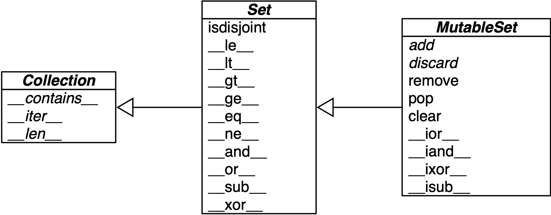
Figure 3-2. Simplified UML class diagram for MutableSet and its superclasses from collections.abc (names in italic are abstract classes and abstract methods; reverse operator methods omitted for brevity)
Tip
The infix operators in Table 3-2 require that both operands be sets, but all other methods take one or more iterable arguments. For example, to produce the union of four collections, a, b, c, and d, you can call a.union(b, c, d), where a must be a set, but b, c, and d can be iterables of any type.
| Math symbol | Python operator | Method | Description |
|---|---|---|---|
S ∩ Z |
|
|
Intersection of |
|
|
Reversed |
|
|
Intersection of |
||
|
|
|
|
|
|
||
S ∪ Z |
|
|
Union of |
|
|
Reversed |
|
|
Union of |
||
|
|
|
|
|
|
||
S Z |
|
|
Relative complement or difference between |
|
|
Reversed |
|
|
Difference between |
||
|
|
|
|
|
|
||
|
Complement of |
||
S ∆ Z |
|
|
Symmetric difference (the complement of the intersection |
|
|
Reversed |
|
|
|
||
|
|
|
Table 3-3 lists set predicates: operators and methods that return True or False.
| Math symbol | Python operator | Method | Description |
|---|---|---|---|
|
|
||
e ∈ S |
|
|
Element |
S ⊆ Z |
|
|
|
|
|
||
S ⊂ Z |
|
|
|
S ⊇ Z |
|
|
|
|
|
||
S ⊃ Z |
|
|
|
In addition to the operators and methods derived from math set theory, the set types implement other methods of practical use, summarized in Table 3-4.
| set | frozenset | ||
|---|---|---|---|
|
● |
Add element |
|
|
● |
Remove all elements of |
|
|
● |
● |
Shallow copy of |
|
● |
Remove element |
|
|
● |
● |
Get iterator over |
|
● |
● |
|
|
● |
Remove and return an element from |
|
|
● |
Remove element |
This completes our overview of the features of sets. As promised in “Dictionary views”, we’ll now see how two of the dictionary view types behave very much like a frozenset.
Set operations on dict views
Table 3-5 shows that the view objects returned by the dict methods .keys() and .items() are remarkably similar to frozenset.
| frozenset | dict_keys | dict_items | Description | |
|---|---|---|---|---|
|
● |
● |
● |
|
|
● |
● |
● |
Reversed |
|
● |
● |
● |
|
|
● |
Shallow copy of |
||
|
● |
Difference between |
||
|
● |
Intersection of |
||
|
● |
● |
● |
|
|
● |
|
||
|
● |
|
||
|
● |
● |
● |
Get iterator over |
|
● |
● |
● |
|
|
● |
● |
● |
|
|
● |
● |
● |
Reversed |
|
● |
● |
Get iterator over |
|
|
● |
● |
● |
Reversed |
|
● |
● |
● |
|
|
● |
Complement of |
||
|
● |
Union of |
||
|
● |
● |
● |
|
|
● |
● |
● |
Reversed |
In particular, dict_keys and dict_items implement the special methods to support
the powerful set operators & (intersection), | (union), - (difference) and ^ (symmetric difference).
This means, for example, that finding the keys that appear in two dictionaries is as easy as this:
>>>d1=dict(a=1,b=2,c=3,d=4)>>>d2=dict(b=20,d=40,e=50)>>>d1.keys()&d2.keys(){'b', 'd'}
Note that the return value of & is a set.
Even better: the set operators in dictonary views are compatible with set instances.
Check this out:
>>>s={'a','e','i'}>>>d1.keys()&s{'a'}>>>d1.keys()|s{'a', 'c', 'b', 'd', 'i', 'e'}
This will save a lot of loops and ifs when inspecting the contents of dictionaries in your code.
We now change gears to discuss how sets and dictionaries are implemented with hash tables. After reading the rest of this chapter, you should no longer be surprised by the behavior of dict, set, and other data structures powered by hash tables.
Internals of sets and dicts
Understanding how Python dictionaries and sets are built with hash tables is helpful to make sense of their strengths and limitations.
Note
Consider this section optional. You don’t need to know all of these details to make good use of dicionaries and sets. But the implementation ideas are beautiful—that’s why I covered them. For practical advice, you can skip to “Practical Consequences of How Sets Work” and “Practical Consequences of How dict Works”.
Here are some questions this section will answer:
-
How efficient are Python
dictandset? -
Why are
setelements unordered? -
Why can’t we use any Python object as a
dictkey orsetelement? -
Why does the order of the
dictkeys depend on insertion order? -
Why does the order of
setelements seem random?
To motivate the study of hash tables, we start by showcasing the amazing performance of dict and set with a simple test involving millions of items.
A Performance Experiment
From experience, all Pythonistas know that dicts and sets are fast. We’ll confirm that with a controlled experiment.
To see how the size of a dict, set, or list affects the performance of search using the in operator, I generated an array of 10 million distinct double-precision floats, the “haystack.” I then generated an array of needles: 1,000 floats, with 500 picked from the haystack and 500 verified not to be in it.
For the dict benchmark, I used dict.fromkeys() to create a dict named haystack with 1,000 floats. This was the setup for the dict test. The actual code I clocked with the timeit module is Example 3-15 (like Example 3-12).
Example 3-15. Search for needles in haystack and count those found
found=0forninneedles:ifninhaystack:found+=1
I repeated the benchmark five times, each time increasing tenfold the size of haystack, from 1,000 to 10,000,000 items. The result of the dict performance test is in Table 3-6.
| len of haystack | Factor | dict time | Factor |
|---|---|---|---|
1,000 |
1× |
0.099ms |
1.00× |
10,000 |
10× |
0.109ms |
1.10× |
100,000 |
100× |
0.156ms |
1.58× |
1,000,000 |
1,000× |
0.372ms |
3.76× |
10,000,000 |
10,000× |
0.512ms |
5.17× |
In concrete terms, to check for the presence of 1,000 floating-point keys in a dictionary with 1,000 items,
the processing time on my laptop was 99µs, and the same search in a dict with 10,000,000 items took 512µs.
In other words, the average time for each search in the haystack with 10 million items was 0.512µs—yes, that’s about half microsecond per needle.
When the search space became 10,000 times larger, the search time increased a little over 5 times. Nice.
To compare with other collections, I repeated the benchmark with the same haystacks of increasing size, but storing the haystack as a set or as list. For the set tests, in addition to timing the for loop in Example 3-15, I also timed the one-liner in Example 3-16, which produces the same result: count the number of elements from needles that are also in haystack—if both are sets.
Example 3-16. Use set intersection to count the needles that occur in haystack
found=len(needles&haystack)
Table 3-7 shows the tests side by side. The best times are in the “set& time” column, which displays results for the set & operator using the code from Example 3-16.
As expected, the worst times are in the “list time” column, because there is no hash table to support searches with the in operator on a list, so a full scan must be made if the needle is not present, resulting in times that grow linearly with the size of the haystack.
| len of haystack | Factor | dict time | Factor | set time | Factor | set& time | Factor | list time | Factor |
|---|---|---|---|---|---|---|---|---|---|
1,000 |
1× |
0.099ms |
1.00× |
0.107ms |
1.00× |
0.083ms |
1.00× |
9.115ms |
1.00× |
10,000 |
10× |
0.109ms |
1.10× |
0.119ms |
1.11× |
0.094ms |
1.13× |
78.219ms |
8.58× |
100,000 |
100× |
0.156ms |
1.58× |
0.147ms |
1.37× |
0.122ms |
1.47× |
767.975ms |
84.25× |
1,000,000 |
1,000× |
0.372ms |
3.76× |
0.264ms |
2.47× |
0.240ms |
2.89× |
8,020.312ms |
879.90× |
10,000,000 |
10,000× |
0.512ms |
5.17× |
0.330ms |
3.08× |
0.298ms |
3.59× |
78,558.771ms |
8,618.63× |
If your program does any kind of I/O, the lookup time for keys in dicts or sets is negligible, regardless of the dict or set size (as long as it fits in RAM). See the code used to generate Table 3-7 and accompanying discussion in [Link to Come], [Link to Come].
Now that we have concrete evidence of the speed of dicts and sets, let’s explore how that is achieved with the help of hash tables.
Set hash tables under the hood
Hash tables are a wonderful invention. Let’s see how a hash table is used when adding elements to a set.
Let’s say we have a set with abbreviated workdays, created like this:
>>>workdays={'Mon','Tue','Wed','Thu','Fri'}>>>workdays{'Tue', 'Mon', 'Wed', 'Fri', 'Thu'}
The core data structure of a Python set is a hash table with at least 8 rows.
Traditionally, the rows in hash table are called buckets8.
A hash table holding the elements of workdays looks like Figure 3-3.
Figure 3-3. Hash table for the set {'Mon', 'Tue', 'Wed', 'Thu', 'Fri'}. Each bucket has two fields: the hash code and a pointer to the element value. Empty buckets have -1 in the hash code field. The ordering looks random.
In CPython built for a 64-bit CPU, each bucket in a set has two fields: a 64-bit hash code, and a 64-bit pointer to the element value—which is a Python object stored elsewhere in memory. Because buckets have a fixed size, access to an individual bucket is done by offset. There is no field for the indexes from 0 to 7 in Figure 3-3.
Before covering the hash table algorithm, we need to know more about hash codes, and how they relate to equality.
Hashes and equality
The hash() built-in function works directly with built-in types and falls back to calling __hash__ for user-defined types. If two objects compare equal, their hash codes must also be equal, otherwise the hash table algorithm does not work. For example, because 1 == 1.0 is True, hash(1) == hash(1.0) must also be True, even though the internal representation of an int and a float are very different.9
Also, to be effective as hash table indexes, hash codes should scatter around the index space as much as possible. This means that, ideally, objects that are similar but not equal should have hash codes that differ widely. Example 3-17 is the output of a script to compare the bit patterns of hash codes. Note how the hashes of 1 and 1.0 are the same, but those of 1.0001, 1.0002, and 1.0003 are very different.
Example 3-17. Comparing hash bit patterns of 1, 1.0001, 1.0002, and 1.0003 on a 32-bit build of Python (bits that are different in the hashes above and below are highlighted with ! and the right column shows the number of bits that differ)
32-bit Python build
1        00000000000000000000000000000001
                                          != 0
1.0      00000000000000000000000000000001
------------------------------------------------
1.0      00000000000000000000000000000001
           ! !!! ! !! ! !    ! ! !! !!!   != 16
1.0001   00101110101101010000101011011101
------------------------------------------------
1.0001   00101110101101010000101011011101
          !!!  !!!! !!!!!   !!!!! !!  !   != 20
1.0002   01011101011010100001010110111001
------------------------------------------------
1.0002   01011101011010100001010110111001
          ! !   ! !!! ! !  !! ! !  ! !!!! != 17
1.0003   00001100000111110010000010010110
------------------------------------------------
The code to produce Example 3-17 is in [Link to Come]. Most of it deals with formatting the output, but it is listed as [Link to Come] for completeness.
Note
Starting with Python 3.3, a random salt value is included when computing hash codes for str, bytes, and datetime objects,
as documented in Issue 13703—Hash collision security issue.
The salt value is constant within a Python process but varies between interpreter runs.
With PEP-456, Python 3.4 adopted the SipHash cryptographic function to compute hash codes for str and bytes objects.
The random salt and SipHash are security measures to prevent DoS attacks.
Details are in a note in the documentation for the __hash__ special method.
Hash collisions
As mentioned, on 64-bit CPython a hash code is a 64-bit number, and that’s 264 possible values—which is more than 1019. But most Python types can represent many more different values. For example, a string made of 10 ASCII printable characters picked at random has 10010 possible values–more than 266. Therefore, the hash code of an object usually has less information than the actual object value. This means that objects that are different may have the same hash code.
Tip
When correctly implemented, hashing guarantees that different hash codes always imply different objects, but the reverse is not true: different objects don’t always have different hash codes. When different objects have the same hash code, that’s a hash collision.
With this basic understanding of hash codes and object equality, we are ready to dive into the algorithm that makes hash tables work, and how hash collisions are handled.
The hash table algorithm
We will focus on the internals of set first, and later transfer the concepts to dict.
Note
This is a simplified view of how Python uses a hash table to implement a set. For all details, see commented source code for CPython’s set and frozenset in Include/setobject.h and Objects/setobject.c.
Let’s see how Python builds a set like {'Mon', 'Tue', 'Wed', 'Thu', 'Fri'}, step by step. The algorithm is illustrated by the flowchart in Figure 3-4, and described next.
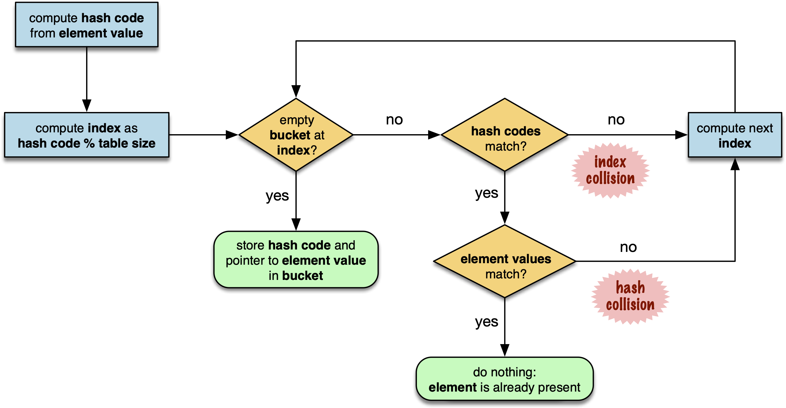
Figure 3-4. Flowchart for algorithm to add element to the hash table of a set.
Step 0: initialize hash table
As mentioned earlier, the hash table for a set starts with 8 empty buckets. As elements are added, Python makes sure at least ⅓ of the buckets are empty—doubling the size of the hash table when more space is needed. The hash code field of each bucket is initialized with -1, which means “no hash code”10.
Step 1: compute the hash code for the element
Given the literal {'Mon', 'Tue', 'Wed', 'Thu', 'Fri'}, Python gets the hash code for the first element, 'Mon'.
For example, here is a realistic hash code for 'Mon'—you’ll probably get a different result because of the random salt Python uses to compute the hash code of strings:
>>>hash('Mon')4199492796428269555
Step 2: probe hash table at index derived from hash code
Python takes the modulus of the hash code with the table size to find a hash table index. Here the table size is 8, and the modulus is 3:
>>>4199492796428269555%83
Probing consists of computing the index from the hash, then looking at the corresponding bucket in the hash table. In this case, Python looks at the bucket at offset 3 and finds -1 in the hash code field, marking an empty bucket.
Step 3: put the element in the empty bucket
Python stores the hash code of the new element, 4199492796428269555, in the hash code field at offset 3, and a pointer to the string object 'Mon' in the element field. Figure 3-5 shows the current state of the hash table.
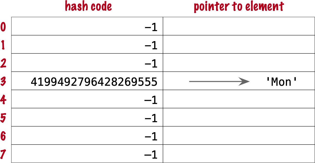
Figure 3-5. Hash table for the set {'Mon'}.
Steps for remaining items
For the second element, 'Tue', steps 1, 2, 3 above are repeated. The hash code for 'Tue' is 2414279730484651250, and the resulting index is 2.
>>>hash('Tue')2414279730484651250>>>hash('Tue')%82
The hash and pointer to element 'Tue' are placed in bucket 2, which was also empty. Now we have Figure 3-6
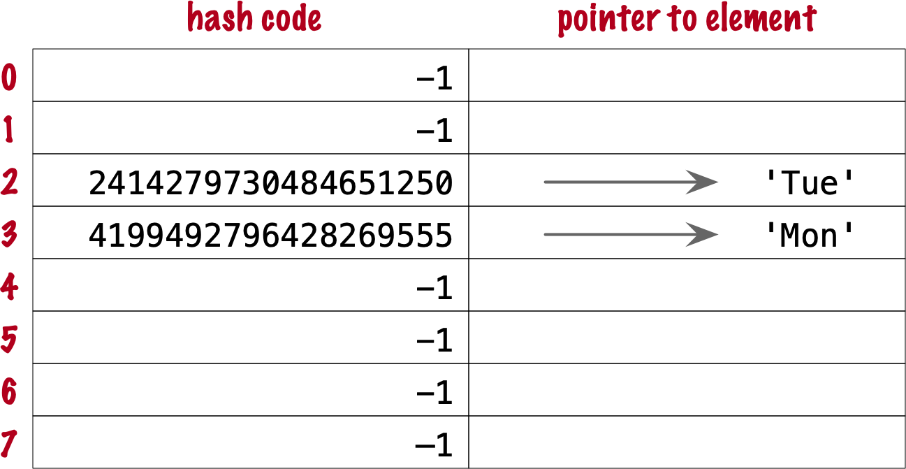
Figure 3-6. Hash table for the set {'Mon', 'Tue'}. Note that element ordering is not preserved in the hash table.
Steps for a collision
When adding 'Wed' to the set, Python computes the hash -5145319347887138165 and index 3.
Python probes bucket 3 and sees that it is already taken. But the hash code stored there, 4199492796428269555 is different.
As discussed in “Hashes and equality”, if two objects have different hashes, then their value is also different.
This is an index collision.
Python then probes the next bucket and finds it empty.
So 'Wed' ends up at index 4, as shown in Figure 3-7.
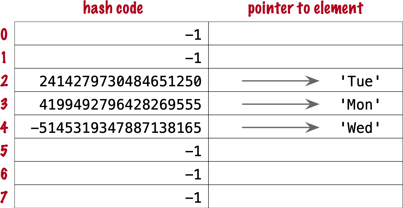
Figure 3-7. Hash table for the set {'Mon', 'Tue', 'Wed'}. After the collision, 'Wed' is put at index 4.
Adding the next element, 'Thu', is boring: there’s no collision, and it lands in its natural bucket, at index 7.
Placing 'Fri' is more interesting.
Its hash, 7021641685991143771 implies index 3, which is taken by 'Mon'. Probing the next bucket—4—Python finds the hash for 'Wed' stored there. The hash codes don’t match, so this is another index collision. Python probes the next bucket. It’s empty, so 'Fri' ends up at index 5. The end state of the hash table is shown in Figure 3-8.
Note
Incrementing the index after a collision is called linear probing. This can lead to clusters of occupied buckets, which can degrade the hash table performance, so CPython counts the number of linear probes and after a certain threshold, applies a pseudo random number generator to obtain a different index from other bits of the hash code. This optimization is particulary important in large sets.
Figure 3-8. Hash table for the set {'Mon', 'Tue', 'Wed', 'Thu', 'Fri'}. It is now 62.5% full—close to the ⅔ threshold.
When there is an element in the probed bucket and the hash codes match, Python also needs to compare the actual object values. That’s because, as explained in “Hash collisions”, it’s possible that two different objects have the same hash code—although that’s rare for strings, thanks to the quality of the Siphash algorithm11. This explains why hashable objects must implement both __hash__ and __eq__.
If a new element were added to our example hash table, it would be more than ⅔ full, therefore increasing the chances of index collisions. To prevent that, Python would alocate a new hash table with 16 buckets, and reinsert all elements there.
All this may seem like a lot of work, but even with millions of items in a set, many insertions happen with no collisions, and the average number of collisions per insertion is between one and two. Under normal usage, even the unluckiest elements can be placed after a handful of collisions are resolved.
Now, given what we’ve seen so far, follow the flowchart in Figure 3-4 to answer the following puzzle without using the computer.
Given the following set, what happens when you add an integer 1 to it?
>>>s={1.0,2.0,3.0}>>>s.add(1)
How many elements are in s now? Does 1 replace the element 1.0?
When you have your answer, use the Python console to verify it.
Searching elements in a hash table
Consider the workdays set with the hash table shown in Figure 3-8.
Is 'Sat' in it? This is the simplest execution path for the expression 'Sat' in workdays:
-
Call
hash('Sat')to get a hash code. Let’s say it is 4910012646790914166 -
Derive a hash table index from the hash code, using
hash_code % table_size. In this case, the index is 6. -
Probe offset 6: it’s empty. This means
'Sat'is not in the set. ReturnFalse.
Now consider the simplest path for an element that is present in the set. To evaluate 'Thu' in workdays:
-
Call
hash('Tue'). Pretend result is 6166047609348267525. -
Compute index:
6166047609348267525 % 8is 5. -
Probe offset 5:
-
Compare hash codes. They are equal.
-
Compare the object values. They are equal. Return
True.
-
Collisions are handled in the way described when adding an element.
In fact, the flowchart in Figure 3-4 applies to searches as well,
with the exception of the terminal nodes—the rectangles with rounded corners.
If an empty bucket is found, the element is not present, so Python returns False;
otherwise, when both the hash code and the values of the sought element match an element in the hash table, the return is True.
Practical Consequences of How Sets Work
The set and frozenset types are both implemented with a hash table, which has these effects:
-
Set elements must be hashable objects. They must implement proper
__hash__and__eq__methods as described in “What Is Hashable?”. -
Membership testing is very efficient. A set may have millions of elements, but the bucket for an element can be located directly by computing the hash code of the element and deriving an index offset, with the possible overhead of a small number of probes to find a matching element or an empty bucket.
-
Sets have a significant memory overhead. The most compact internal data structure for a container would be an array of pointers12. Compared to that, a hash table adds a hash code per entry, and at least ⅓ of empty buckets to minimize collisions.
-
Element ordering depends on insertion order, but not in a useful or reliable way. If two elements are involved in a collision, the bucket were each is stored depends on which element is added first.
-
Adding elements to a set may change the order of other elements. That’s because, as the hash table is filled, Python may need to recreate it to keep at least ⅓ of the buckets empty. When this happens, elements are reinserted and different collisions may occur.
Hash table usage in dict
Since 2012, the implementation of the dict type had two major optimizations to reduce memory usage.
The first one was proposed as PEP 412 — Key-Sharing Dictionary and implemented in Python 3.313.
The second is called “compact dict", and landed in Python 3.6.
As a side effect, the compact dict space optimization preserves key insertion order.
In the next sections we’ll discuss the compact dict and the new key-sharing scheme—in this order, for easier presentation.
How compact dict saves space
Note
This is a high level explanation of the Python dict implementation.
One difference is that the actual usable fraction of a dict hash table is ⅓, and not ⅔ as in sets.
The actual ⅓ fraction would require 16 buckets to hold the 4 items in my example dict,
and the diagrams in this section would become too tall, so I pretend the usable fraction is ⅔ in these explanations.
One comment in Objects/dictobject.c
explains that any fraction between ⅓ and ⅔ “seem to work well in practice”.
Consider a dict holding the abbreviated names for the weekdays from 'Mon' through 'Thu', and the number of students enrolled in swimming class on each day:
>>>swimmers={'Mon':14,'Tue':12,'Wed':14,'Thu':11}
Before the compact dict optimization, the hash table underlying the swimmers dictionary would look like Figure 3-9.
As you can see, in a 64-bit Python, each bucket holds three 64-bit fields:
the hash code of the key, a pointer to the key object, and a pointer to the value object.
That’s 24 bytes per bucket.

Figure 3-9. Old hash table format for a dict with 4 key-value pairs. Each bucket is a struct with the hash code of the key, a pointer to the key, and a pointer to the value.
The first two fields play the same role as they do in the implementation of sets.
To find a key, Python computes the hash code of the key, derives an index from the key,
then probes the hash table to find a bucket with a matching hash code and a matching key object.
The third field provides the main feature of a dict: mapping a key to an arbitrary value.
The key must be a hashable object, and the hash table algorithm ensures it will be unique in the dict.
But the value may be any object—it doesn’t need to be hashable or unique.
Raymond Hettinger observed that significant savings could be made if the hash code and pointers to key and value were held in an entries array with no empty rows,
and the actual hash table were a sparse array with much smaller buckets holding indexes into the entries array14.
In his original message to python-dev,
Hettinger called the hash table indices. The width of the buckets in indices varies as the dict grows, starting at 8-bits per bucket—enough to index up to 128 entries, while reserving negative values for special purposes, such as -1 for empty and -2 for deleted.
As an example, the swimmers dictionary would then be stored as shown in Figure 3-10.
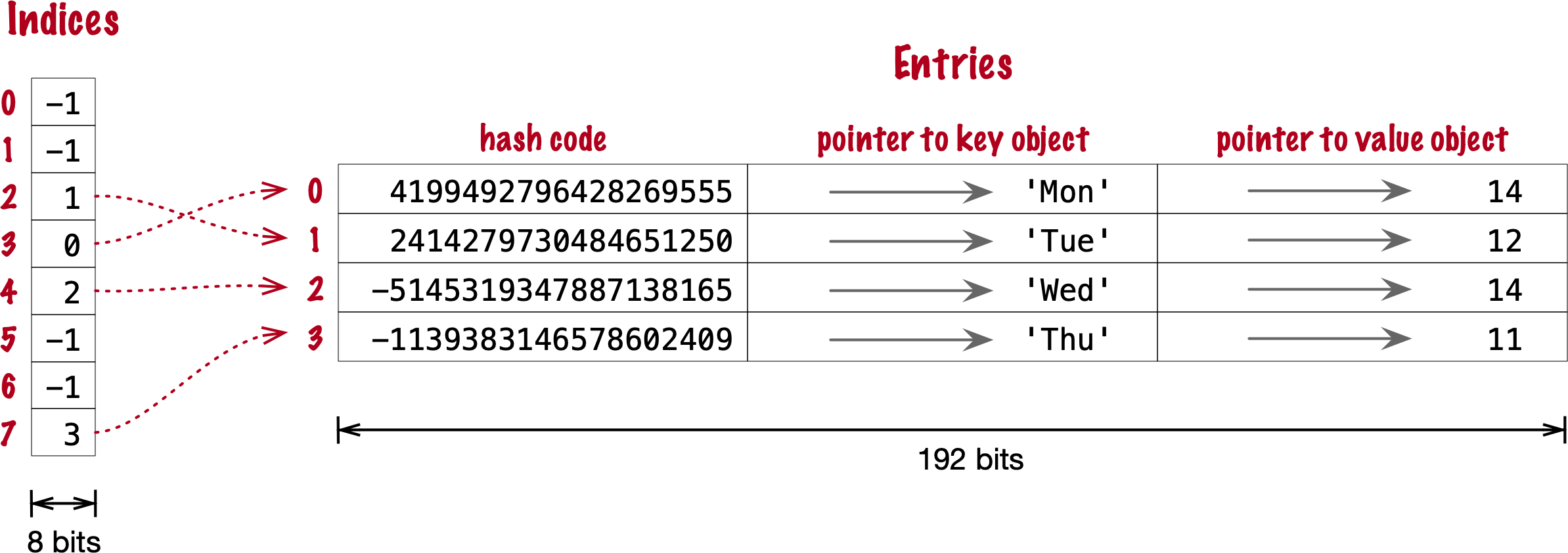
Figure 3-10. Compact storage for a dict with 4 key-value pairs. Hash codes and pointers to keys and values are stored in insertion order in the entries array, and the entry offsets derived from the hash codes are held in the indices sparse array, where an index value of -1 signals an empty bucket.
Assuming a 64-bit build of CPython, our 4-item swimmers dictionary would take 192 bytes of memory in the old scheme:
24 bytes per bucket, times 8 rows.
The equivalent compact dict uses 104 bytes in total: 96 bytes in entries (24 * 4),
plus 8 bytes for the buckets in indices—configured as an array of 8 bytes.
The next section describes how those two arrarys are used.
Algorithm for adding items to compact dict.
Step 0: set up indices
The indices table is initially set up as an array of signed bytes, with 8 buckets, each initialized with -1 to signal “empty bucket”.
Up to 5 of these buckets will eventually hold indices to rows in the entries array, leaving ⅓ of them with -1.
The other array, entries, will hold key/value data with the same three fields as in the old scheme—but in insertion order.
Step 1: compute hash code for the key
To add the key-value pair ('Mon', 14) to the swimmers dictionary,
Python first calls hash('Mon') to compute the hash code of that key.
Step 2: probe entries via indices
Python computes hash('Mon') % len(indices). In our example, this is 3.
Offset 3 in indices holds -1: it’s an empty bucket.
Step 3: put key-value in entries, updating indices.
The entries array is empty, so the next available offset there is 0.
Python puts 0 at offset 3 in indices and stores
the hash code of the key, a pointer to the key object 'Mon', and a pointer to the int value 14
at offset 0 in entries.
Figure 3-11 shows the state of the arrays when the value of swimmers is {'Mon': 14}.

Figure 3-11. Compact storage for the {'Mon': 14}: indices[3] holds the offset of the first entry: entries[0].
Steps for next item
To add ('Tue', 12) to swimmers:
-
Compute hash code of key
'Tue'. -
Compute offset into
indices, ashash('Tue') % len(indices). This is 2.indices[2]has -1. No collision so far. -
Put the next available
entriesoffset, 1, inindices[2], then store entry atentries[1].
Now the state is Figure 3-12. Note that entries holds the key-value pairs in insertion order.

Figure 3-12. Compact storage for the {'Mon': 14, 'Tue': 12}.
Steps for a collision
-
Compute hash code of key
'Wed'. -
Now,
hash('Wed') % len(indices)is 3.indices[3]has 0, pointing to an existing entry. Look at the hash code inentries[0]. That’s the hash code for'Mon', which happens to be different than the hash code for'Wed'. This mismatch signals a collision. Probes the next index:indices[4]. That’s -1, so it can be used. -
Make
indices[4] = 2, because 2 is the next available offset atentries. Then fillentries[2]as usual.
After adding ('Wed', 14), we have Figure 3-13
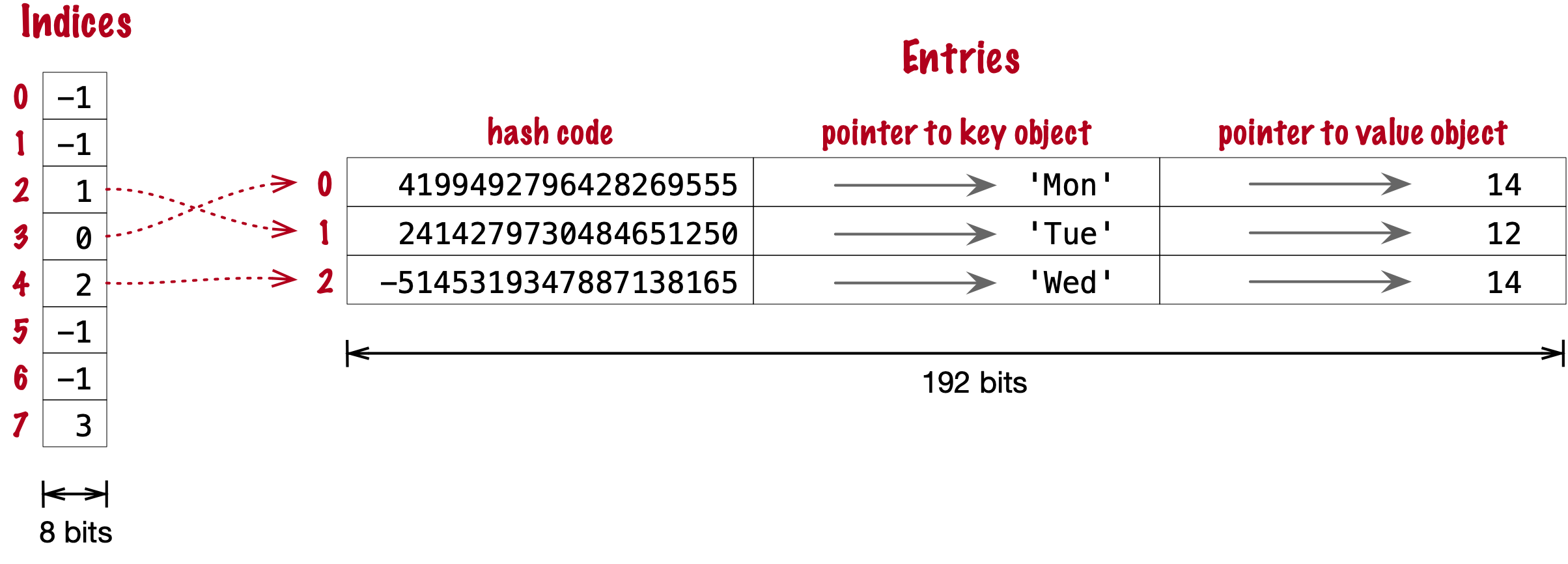
Figure 3-13. Compact storage for the {'Mon': 14, 'Tue': 12, 'Wed': 14}.
How a compact dict grows
Recall that the buckets in the indices array are 8 signed bytes initially, enough to hold offsets for up to 5 entries, leaving ⅓ of the buckets empty.
When the 6th item is added to the dict, indices is reallocated to 16 buckets—enough for 10 entry offsets.
The size of indices is doubled as needed, while still holding signed bytes, until the time comes to add the 129th item to the dict.
At this point, the indices array has 256 8-bit buckets. However, a signed byte is not enough to hold offsets after 128 entries,
so the indices array is rebuilt to hold 256 16-bit buckets to hold signed integers—wide enough to represent offsets to 32,768 rows in the entries table.
The next resizing happens at the 171st addition, when indices would become more than ⅔ full.
Then the number of buckets in indices is doubled to 512, but each bucket still 16-bits wide each.
In summary, the indices array grows by doubling the number of buckets,
and also—less often—by doubling the width of eack bucket to accomodate a growing number of rows in entries.
This concludes our summary of the compact dict implementation.
I ommited many details, but now let’s take a look at the other space-saving optimization for dictionaries: key-sharing.
Key-sharing dictionary
Instances of user-defined classes usually hold their attributes in a __dict__
attribute which is a regular dictionary15.
In an instance __dict__, the keys are the attribute names, and the values are the attribute values.
Most of the time, all instances have the same attributes with different values.
When that happens, 2 of the 3 fields in the entries table for every instance has the exact same content:
the hash code of the attribute name, and a pointer to the attribute name.
Only the pointer to the attribute value is different.
In PEP 412 — Key-Sharing Dictionary,
Mark Shannon proposed to split the storage of dictionaries used as instance __dict__,
so that each attribute hash code and pointer is stored only once, linked to the class,
and the attribute values are kept in parallel arrays of pointers attached to each instance.
Given a Movie class where all instances have the same attributes named
'title', 'release', 'directors', and 'actors',
Figure 3-14 shows the arrangement of key-sharing in a split
dictionary—also implemented with the new compact layout.
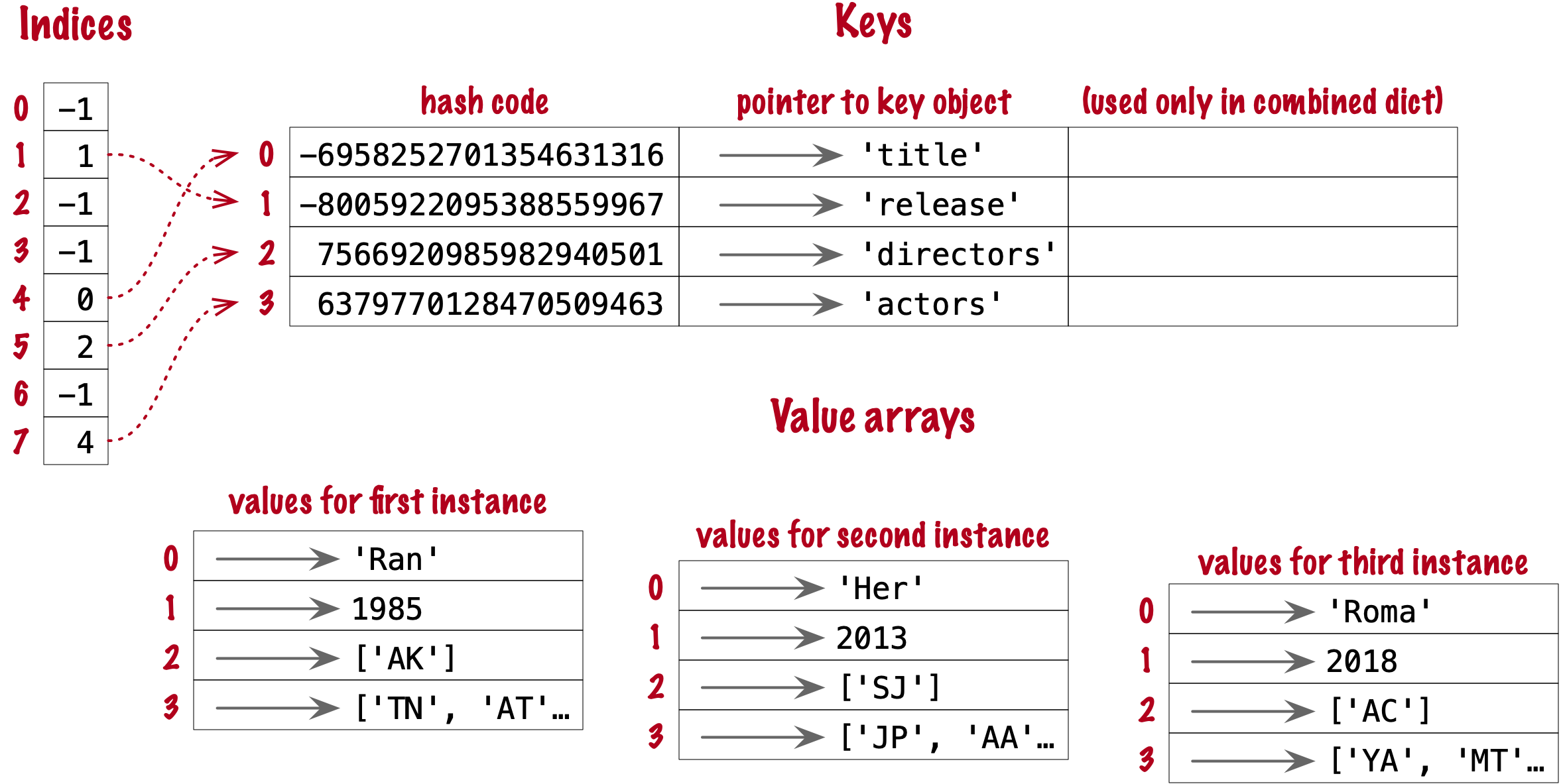
Figure 3-14. Split storage for the __dict__ of a class and three instances.
PEP 412 introduced the terms combined-table to discuss the old layout and and split-table for the proposed optimization.
The combined-table layout is still the default when you create a dict using literal syntax or call dict().
A split-table dictionary is created to fill the __dict__ special attribute of an instance, when it is the first instance of a class.
The keys table (see Figure 3-14) is then cached in the class object.
This leverages the fact that most Object Oriented Python code assigns all instance attributes in the __init__ method.
That first instance (and all instances after it) will hold only its own a value array.
If an instance gets a new attribute not found in the shared keys table, then this instance’s __dict__ is converted to combined-table form.
However, if this instance is the only one in its class, the __dict__ is converted back to split-table,
since it is assumed that further instances will have the same set of attributes and key sharing will be useful.
The PyDictObject struct that represents a dict in the CPython source code is the same for both combined-table and split-table dictionaries.
When a dict converts from one layout to the other, the change happens in PyDictObject fields,
with the help of other internal data structures.
Practical Consequences of How dict Works
-
Keys must be hashable objects. They must implement proper
__hash__and__eq__methods as described in “What Is Hashable?”. -
Key searches are nearly as fast as element searches in sets.
-
Item ordering is preserved in the
entriestable—this was implemented in CPython 3.6, and became an official language feature in 3.7. -
To save memory, avoid creating instance attributes outside of the
__init__method. If all instance attributes are created in__init__, the__dict__of your instances will use the split-table layout, sharing the same indices and key entries array stored with the class.
Chapter Summary
Dictionaries are a keystone of Python. Beyond the basic dict, the standard library offers handy, ready-to-use specialized mappings like defaultdict, ChainMap, and Counter, all defined in the collections module. With the new dict implementantion, OrderedDict is not as useful as before, but should remain in the standard library for backward-compatibility—and it offers the .popitem(last=False) method option to drop and return the first item, which dict doesn’t yet have. Also in the collections module is the easy-to-extend UserDict class.
Two powerful methods available in most mappings are setdefault and update. The setdefault method is used to update items holding mutable values, for example, in a dict of list values, to avoid redundant searches for the same key. The update method allows bulk insertion or overwriting of items from any other mapping, from iterables providing (key, value) pairs and from keyword arguments. Mapping constructors also use update internally, allowing instances to be initialized from mappings, iterables, or keyword arguments.
A clever hook in the mapping API is the __missing__ method, which lets you customize what happens when a key is not found when using the d[k] syntax which invokes __getitem__.
The collections.abc module provides the Mapping and MutableMapping abstract base classes as standard interfaces, useful for run-time type checking. The little-known MappingProxyType from the types module creates immutable mappings. There are also ABCs for Set and MutableSet.
Dictionary views are a great addition in Python 3, without the memory overhead of the Python 2 .keys(), .values() and .items() methods that built lists duplicating data in the target dict instance. In addition, the dict_keys and dict_items classes support the most useful methods and operators of frozenset.
The hash table implementation underlying set is extremely fast. Understanding its logic explains why elements are apparently unordered and may even be reordered behind our backs. There is a price to pay for all this speed, and the price is in memory. Finally, we saw how optimizations in the hash tables underlying dict save memory and preserve key insertion order.
Further Reading
In The Python Standard Library documentation, 8.3. collections — Container datatypes includes examples and practical recipes with several mapping types. The Python source code for the module Lib/collections/__init__.py is a great reference for anyone who wants to create a new mapping type or grok the logic of the existing ones. Chapter 1 of Python Cookbook, Third edition (O’Reilly) by David Beazley and Brian K. Jones has 20 handy and insightful recipes with data structures—the majority using dict in clever ways.
Greg Gandenberger advocates for the continued use of collections.Orderedict, on the grounds that “explicit is better than implicit”, backward compatibility, and the fact that some tools and libraries assume the ordering of dict keys is irrelevant—his post: Python Dictionaries Are Now Ordered. Keep Using OrderedDict..
PEP 3106 — Revamping dict.keys(), .values() and .items() is where Guido van Rossum presented the dictionary views feature for Python 3. In the abstract, he wrote the idea came the Java Collections Framework.
Pypy was the first Python interpreter to implement Raymond Hettinger’s proposal of compact dicts, and they blogged about it in Faster, more memory efficient and more ordered dictionaries on PyPy, acknowledging that a similar layout was adopted in PHP 7, descibed in PHP’s new hashtable implementation. It’s always great when creators cite prior art.
At PyCon 2017, Brandon Rhodes presented The Dictionary Even Mightier, a sequel to his classic animated presentation The Mighty Dictionary—including animated hash collisions!
Another up-to-date, but more in-depth video on the internals of Python’s dict is Modern Dictionaries
by Raymond Hettinger, where he tells that after initially failing to sell compact dicts to the CPython core devs, he lobbied the Pypy team, they adopted it,
the idea gained traction, and was finally contributed to CPython 3.6 by by INADA Naoki.
For all details, check out the extensive comments in the CPython code for Objects/dictobject.c and Objects/dict-common.h, as well as the design document Objects/dictnotes.txt.
The rationale for adding sets to Python is documented in PEP 218 — Adding a Built-In Set Object Type. When PEP 218 was approved, no special literal syntax was adopted for sets. The set literals were created for Python 3 and backported to Python 2.7, along with dict and set comprehensions. At PyCon 2019, I presented Set Practice: learning from Python’s set types (slides), describing use cases of sets in real programs, covering their API design, and the implementantion of uintset, a set class for integer elements using a bit vector instead of a hash table, inspired by an example in chapter 6 of the excellent The Go Programming Language, by Donovan & Kernighan.
IEEE’s Spectrum magazine has a story about Hans Peter Luhn, a prolifc inventor who patented a punched card deck to select cocktail recipes depending on ingredients available, among other diverse inventions including… hash tables! See in Hans Peter Luhn and the Birth of the Hashing Algorithm.
1 PyCon 2017 talk; video available at https://youtu.be/66P5FMkWoVU?t=56
2 The original script appears in slide 41 of Martelli’s “Re-learning Python” presentation. His script is actually a demonstration of dict.setdefault, as shown in our Example 3-4.
3 This is an example of using a method as a first-class function, the subject of Chapter 7.
4 One such library is Pingo.io, no longer under active development.
5 The exact problem with subclassing dict and other built-ins is covered in [Link to Come].
6 Dictionary views were backported to Python 2.7 and are returned by the dict methods .viewkeys(), .viewvalues(), and .viewitems(). I hope this information is of no use to you, dear reader, as Python 2.7 is now history.
7 This may be interesting, but is not super important. The speed up will happen only when a set literal is evaluated, and that happens at most once per Python process—when a module is initially compiled. If you’re curious, import the dis function from the dis module and use it to disassemble the bytecodes for a set literal—e.g. dis('{1}')—and a set call—dis('set([1])')
8 The word “bucket” makes more sense to describe hash tables that hold more than one element per row. Python stores only one element per row, but we will stick with the colorful traditional term.
9 Since I just mentioned int, here is a CPython implementation detail: the hash code of an int that fits in a machine word is the value of the int itself, except the hash code of -1, which is -2.
10 The hash() built-in never returns -1 for any Python object. If x.__hash__() returns -1, hash(x) returns -2.
11 On 64-bit CPython, string hash collisions are so uncommon that I was unable to produce an example for this explanation. If you find one, let me know.
12 That’s how tuples are stored.
13 That was before I started writing the 1st edition of Fluent Python, but I missed it.
14 It’s ironic that the buckets in the hash table here do not contain hash codes, but only indexes to the entries array where the hash codes are. But, conceptually, the index array is really the hash table in this implementation, even if there are no hashes in its buckets.
15 Unless the class has a __slots__ atribute, as we’ll see in chapter XXX
16 Quoted in Butler Lampson’s Turing lecture slides Principles for Computer System Design