
Chapter 13
Managing and monitoring SQL Server
Maintaining indexes and statistics
Maintaining database file sizes
Monitoring databases by using DMVs
Capturing Windows performance metrics with DMVs and data collectors
Chapter 11 discusses the importance and logistics of database backups, but what else do you need to do on a regular basis to maintain a healthy SQL Server? In this chapter, we lay the foundation for the what and why of Microsoft SQL Server management, including key dynamic management views (DMVs) along the way, and how to set up extended events (the replacement for traces). We review what to look for in the Windows Performance Monitor for SQL Server instances and Database Transaction Unit (DTU) metrics for databases in Microsoft Azure SQL Database. Finally, we review the major changes to the SQL Server servicing model. For example, there are no more service packs: it’s cumulative updates from here out.
Detecting database corruption
Aside from database backups, the second most important factor concerning database page integrity is the proper configuration to prevent, and the monitoring to mitigate, database corruption. This isn’t a complicated topic and mostly revolves around one setting and one command.
Setting the database’s page verify option
For all databases, this setting should be CHECKSUM. The legacy TORN_PAGE option is a sign that this database has been moved over the years, up from a pre–SQL 2005 version, but this setting has never changed. Since SQL 2005, CHECKSUM has the superior and default setting, but it requires an Administrator to manually change after a database is restored up.
If you still have databases with a page verify option that is not CHECKSUM, you should change this setting immediately.
![]() For more information on database files and filegroups, see Chapter 3.
For more information on database files and filegroups, see Chapter 3.
Using DBCC CHECKDB
You should periodically run CHECKDB on all databases. This is a time-consuming but crucial process. You should run DBCC CHECKDB at least as often as your backup retention plan, and consider DBCC CHECKDB nearly as important as regular database backups. It’s worth noting that the only reliable solution to database corruption is restoring from a known good backup.
For example, if you keep local backups around for one month, you should ensure that you perform a successful DBCC CHECKDB no less than once per month. More often as possible is recommended, of course. This ensures that you will at least have a recovery point for uncorrupted, unchanged data, and a starting point for corrupted data fixes. On large databases, DBCC CHECKDB could take hours and block other user queries.
The DBCC CHECKDB command actually covers other more-granular database integrity check tasks, including DBCC CHECKALLOC, DBCC CHECKTABLE, or DBCC CHECKCATALOG, all of which are important, and in only rare cases need to be run separately or to split up the workload.
Running DBCC CHECKDB, with no other parameters or syntax, performs a database integrity test on the current database context. Without specifying a database, however, no other additional options can be provided. There are a number of parameters for CHECKDB detailed at
https://docs.microsoft.com/sql/t-sql/database-console-commands/dbcc-checkdb-transact-sql.
Here are some parameters worth noting:
NOINDEX. This can reduce the duration of the integrity check by ignoring nonclustered rowstore and Columnstore indexes.
Example usage:
DBCC CHECKDB (databasename, NOINDEX);
NO_INFOMSGS. This suppresses informational status messages and returns only errors.
Example usage:
DBCC CHECKDB (databasename) WITH NO_INFOMSGS;
REPAIR_REBUILD. You should run this only as a last resort because although it might have some success, it is unlikely to result in a complete repair. It can also be very time consuming, involving the rebuilding of indexes based on attempted repair data. We suggest that you review the
DBCC CHECKDBdocumentation for a number of caveats.Example usage:
DBCC CHECKDB (databasename) WITH REPAIR_REBUILD;
REPAIR_ALLOW_DATA_LOSS. You should run this only as a last resort to achieve a partial database recovery because it could force a database to resolve errors by simply deallocating pages, potentially creating gaps in rows or columns. You must run this in
SINGLE_USERmode, and you should run it inEMERGENCYmode. Review theDBCC CHECKDBdocumentation for a number of caveats. A complete review of howEMERGENCYmode andREPAIR_ALLOW_DATA_LOSSis detailed in this blog post by Paul Randal: https://www.sqlskills.com/blogs/paul/checkdb-from-every-angle-emergency-mode-repair-the-very-very-last-resort/.Example usage: (last resort only, not recommended!)
ALTER DATABASE WorldWideImporters SET EMERGENCY, SINGLE_USER;
DBCC CHECKDB('WideWorldImporters', REPAIR_ALLOW_DATA_LOSS);
ALTER DATABASE WorldWideImporters SET MULTI_USER;ESTIMATEONLY. This does not provide an estimate of the duration of a
CHECKDB(without other parameters), only an amount of space required in TempDB.Example usage:
DBCC CHECKDB (databasename) WITH ESTIMATEONLY;
These scripts are all available in the accompanying downloads for this book at https://aka.ms/SQLServ2017Admin/downloads.
![]() For more information on automating DBCC CHECKDB, see Chapter 14.
For more information on automating DBCC CHECKDB, see Chapter 14.
Repairing database data file corruption
Of course, the only real remedy to data corruption after it has happened is by restoring from a backup. The well-documented DBCC CHECKDB REPAIR_ALLOW_DATA_LOSS should be a last resort.
It is possible to repair missing pages in clustered indexes by piecing together missing columns in nonclustered indexes. In reality, this is an academic solution because data corruption rarely happens in such a tidy and convenient way.
Always On availability groups also provide a built-in data corruption detection and automatic repair capability by using uncorrupted data on one replica to replace inaccessible data on another.
![]() For more information on this feature of availability groups, see Chapter 12.
For more information on this feature of availability groups, see Chapter 12.
Recovering the database transaction log file corruption
In addition to the previous guidance on the importance of backups, you can reconstitute a corrupted or lost database transaction log file (though not recovered) by using the example that follows. A lost transaction log file will likely result in the loss of some recent rows, but in the event of a disaster recovery involving the loss of the .ldf file but an intact .mdf file, this could be a valuable step.
It is possible to rebuild a blank transaction log file in a new file location for a database by using the following command:
ALTER DATABASE WorldWideImporters SET EMERGENCY, SINGLE_USER;
ALTER DATABASE WorldWideImporters REBUILD LOG
ON (NAME=WWI_Log, FILENAME='F:DATAWideWorldImporters_new.ldf');
ALTER DATABASE WorldWideImporters SET MULTI_USER;
These scripts are all available in the accompanying downloads for this book, which are available at https://aka.ms/SQLServ2017Admin/downloads.
Database corruption in databases in Azure SQL Database
Microsoft takes data integrity in its platform-as-a-service (PaaS) database offering very seriously and provides strong assurances of assistance and recovery for its product. Albeit rare, Azure engineering teams respond 24x7 globally to data corruption reports. The Azure SQL Database engineering team details its response promises at https://azure.microsoft.com/blog/data-integrity-in-azure-sql-database/.
Maintaining indexes and statistics
Maintaining index fragmentation is about proper organization of rowstore data within the file that SQL Server maintains, minimizing the number of pages that must be read when queries read or write those data pages. Reducing fragmentation in database objects is vastly different from reducing fragmentation at the drive level and has little in common with the Disk Defragmenter application of Windows. Although this doesn’t translate to page locations on magnetic disks (and on Storage-Area Networks, this has even less relevance), it does translate to the activity of I/O systems when retrieving data.
The causes of index fragmentation are, to be put plainly, writes. Our data would stay nice and tidy if applications would stop writing to it! There will inevitably be a significant effect that updates and deletes have on clustered and nonclustered index fragmentation, plus the effect that inserts could have on fragmentation because of clustered index design.
The information in this section is largely unchanged and applies to SQL Server instances, databases in Azure SQL Database, and even Azure SQL Data Warehouse. (All tables in Azure SQL Data Warehouse have a Columnstore clustered index by default.)
Changing the Fill Factor property when beneficial
Each rowstore index on disk-based objects has a numeric property called Fill Factor that specifies the percentage of space to be filled with rowstore data in each leaf-level data page of the index when it is created or rebuilt. The instance-wide default Fill Factor is 0%, which is the same as 100%; that is each leaf-level data page will be completely filled. A Fill Factor of 80 means that 20% of leaf-level data pages will be intentionally left empty. We can adjust this Fill Factor percentage for each index to manage the efficiency of data pages.
A low Fill Factor will help reduce the number page splits, which occur when the Database Engine attempts to add a new row of data or update an existing row with more data to a page that is already full. In this case, the Database Engine will clear out space for the new row by moving a proportion of the old rows to a new page. This can be a time- and resource-consuming operation, with many page splits possible during writes, and will lead to index fragmentation.
However, setting a low Fill Factor will greatly increase the number of pages needed to store the same data and increase the number of reads during query operations. For example, a Fill Factor of 50 will roughly double the space on the drive that it initially takes to store and therefore access the data, when compared to a Fill Factor of 0 or 100.
In most instances, data is read far more often that it is written and inserted, updated, and deleted upon occasion. Indexes will therefore benefit from a high Fill Factor, almost always more than 80, because it is more important to keep the number of reads to a manageable level than minimizing the resources needed to perform a page split. You can deal with the index fragmentation by using the REBUILD or REORGANIZE commands, as discussed in the next section.
If the key value for an index is constantly increasing, such as an autoincrementing IDENTITY column as the first key of a clustered index, the data would always be added to the end of a data page and any gaps would not need to be filled. In the case of a table for which data is always inserted sequentially and never updated, setting a Fill Factor other than the default of 0/100 will have no benefits. (It is still possible.) Even after fine tuning a Fill Factor, you might not find that the benefit of reducing page splits has any noticeable benefit to write performance.
You can set a Fill Factor when an index is first created, or you can change it by using the ALTER INDEX … REBUILD syntax, as discussed in the next section.
Tracking page splits
If you are intent on fine-tuning the Fill Factor for important tables to maximize the performance/storage space ratio, you can measure page splits in two ways.
You can use the performance counter DMV to measure page splits in aggregate on Windows server, as shown here:
SELECT * FROM sys.dm_os_performance_counters WHERE counter_name ='Page Splits/sec'
The cntr_value will increment whenever a page split is detected. This is a bit misleading because to calculate the page splits per second, you must sample the incrementing value twice, and divide by the time difference between the samples. When viewing this metric in Performance Monitor, the math is done for you.
Using extended events session to identify page_split events
You can track page_split events alongside statement execution by adding the page_split event to sessions such as the Transact-SQL (T-SQL) template in the extended events wizard.
We review extended events and the sys.dm_os_performance_counters DMV later in this chapter, including a sample session script to track page_split events.
Monitoring index fragmentation
You can find the extent to which an index is fragmented by interrogating the sys.dm_db_index_physical_stats dynamic management function (DMF). Be aware that unlike most DMVs, this function can have a significant impact on server performance because it can tax I/O.
To query this DMF, you must be a member of the sysadmin server role, or the db_ddladmin and db_owner database roles. Alternatively, you can grant CONTROL permission to the object, then also the VIEW DATABASE STATE and VIEW SERVER STATE permissions. For more information, refer to https://docs.microsoft.com/sql/relational-databases/system-dynamic-management-views/sys-dm-db-index-physical-stats-transact-sql#permissions.
Keep this in mind when scripting this operation for automated index maintenance. We discuss more about automating index maintenance in Chapter 14.
For example, to find the fragmentation level of all indexes on the Sales.Orders table in the WideWorldImporters sample database, we could use a query such as the following:
SELECT
DB = db_name(s.database_id)
, [schema_name] = sc.name
, [table_name] = o.name
, index_name = i.name
, s.index_type_desc
, s.partition_number -- if the object is partitioned
, avg_fragmentation_pct = s.avg_fragmentation_in_percent
, s.page_count -- pages in object partition
FROM sys.indexes AS i
CROSS APPLY sys.dm_db_index_physical_stats (DB_ID(),i.object_id,i.index_id, NULL, NULL) AS s
INNER JOIN sys.objects AS o ON o.object_id = s.object_id
INNER JOIN sys.schemas AS sc ON o.schema_id = sc.schema_id
WHERE i.is_disabled = 0
AND o.object_id = OBJECT_ID('Sales.Orders');
The sys.dm_db_index_physical_stats DMF accepts five parameters: database_id, object_id, index_id, partition_id, and mode. The mode parameters default to LIMITED, the fastest method, but you can set it to Sampled and Detailed. These additional modes are rarely necessary, but they provide more data and more-precise data. Some columns will be NULL in LIMITED mode. For the purposes of determining fragmentation, the default mode of LIMITED (used when the parameter value of NULL is provided) suffices.
The five parameters of the sys.dm_db_index_physical_stats DMF are all nullable. For example, if you run
SELECT * FROM sys.dm_db_index_physical_stats(NULL,NULL,NULL,NULL,NULL);
you will see fragmentation statistics for all databases, all objects, all indexes, and all partitions.
We recommend that you do not do this; again, because this can have a significant impact on server resources resulting in a noticeable drop in performance. The previous sample scripts are all available in the accompanying downloads for this book, which are available at https://aka.ms/SQLServ2017Admin/downloads.
Rebuilding indexes
Performing an INDEX REBUILD operation on a rowstore index (clustered or nonclustered) will physically re-create the index b-tree leaf level. The goal of moving the pages is to make storage more efficient and to match the logical order provided by the index key. A rebuild operation is both destructive to the index object and will block other queries attempting to access the pages. Because the rebuild operation destroys and re-creates the index, it must update the index statistics afterward, eliminating the need to perform a subsequent UPDATE STATISTICS operation as part of regular maintenace.
Long-term table locks are held during the rebuild operation. One of the major advantages of SQL Server Enterprise edition remains the ability to specify the ONLINE keyword, which allows for rebuild operations to be significantly less disruptive to other queries (though not completely), making feasible index maintenance on SQL Servers with round-the-clock activity.
You should use ONLINE with index rebuild operations whenever possible, if time allows. An ONLINE index rebuild might take longer than an offline rebuild, however. There are also scenarios for which an ONLINE rebuild is not possible, including deprecated data types image, text and ntext, or the xml data type. Since SQL Server 2012, it is possible to perform ONLINE index rebuilds on the MAX lengths of the data types varchar, nvarchar, and varbinary.
For the syntax to rebuild the FK_Sales_Orders_CustomerID nonclustered index on the Sales.Orders table with the ONLINE functionality in Enterprise edition, see the following code sample:
ALTER INDEX FK_Sales_Orders_CustomerID
ON Sales.Orders
REBUILD WITH (ONLINE=ON);
It’s important to note that if you perform any kind of index maintenance on the clustered index of a rowstore table, it does not affect the nonclustered indexes. Nonclustered indexes fragmentation will not change if you rebuild the clustered index, and must be maintained, as well. However, dropping and re-creating the clustered index will require the nonclustered indexes to be rebuilt twice: once to change the nonclustered indexes to reference a heap, and again to reference the new clustered index.
Instead of rebuilding an individual index, you can instead rebuild all indexes on a particular table by replacing the name of the index with the keyword ALL. This is usually overkill and inefficient, and individual index operations when needed are preferred. For example, to rebuild all indexes on the Sales.Orders table, do the following:
ALTER INDEX ALL ON Sales.Orders REBUILD;
You can also do this in SQL Server Management Studio. To do so, under the Sales.Order table, expand the Indexes folder. Right-click the FK_Sales_Orders_CustomerID index, and then, on the shortcut menu that opens, select Rebuild. Note, though, that you cannot specify options such as ONLINE in this dialog box. (Note also that the right-click shortcut options to Rebuild or Reorganize are unavailable for indexes on memory-optimized tables.)
Aside from ONLINE, there are other options that you might want to consider for INDEX REBUILD operations. Let’s take a look at them:
SORT_IN_TEMPDB. Use this when you want to create or rebuild an index using TempDB for sorting the index data, potentially increasing performance by distributing the I/O activity across multiple drives. This also means that these sorting work tables are written to the TempDB database transaction log instead of the user database transaction log, potentially reducing the log impact on the user database and allowing for the user database transaction log to be backed up during the operation.
MAXDOP. You can use this to mitigate some of the impact of index maintenance by preventing the operation from using parallel processors. This can cause the index maintenance operation to run longer, but to have less impact on performance.
WAIT_AT_LOW_PRIORITY. Introduced in SQL Server 2014, this is the first of a set of parameters that you can use to instruct the
ONLINEindex maintenance operation to try not to block other operations, and how. This feature is known as Managed Lock Priority, and this syntax is not usable outside of online index operations and partition switching operations. Here is the full syntax:ALTER INDEX FK_Sales_Orders_CustomerID ON Sales.Orders
REBUILD WITH (ONLINE=ON (WAIT_AT_LOW_PRIORITY (MAX_DURATION = 0 MINUTES,
ABORT_AFTER_WAIT = SELF)));The parameters for
MAX_DURATIONandABORT_AFTER_WAITinstruct the statement how to proceed if it begins to be blocked by another operation. The online index operation will wait, allowing other operations to proceed.The
MAX_DURATIONparameter can be 0 (wait indefinitely) or a measure of time in minutes (no other unit of measure is supported)The
ABORT_AFTER_WAITparameter provides an action at the end of theMAX_DURATIONwait:SELFinstructs the statement to terminate its own process, ending the online rebuild step.BLOCKERSinstructs the statement to terminate the other process that is being blocked, terminating what is potentially a user transactions. Use with caution.NONEinstructs the statement to continue to wait, and when combined withMAX_DURATION = 0, essentially the same behavior as not specifyingWAIT_AT_LOW_PRIORITY.
RESUMABLE. Introduced in SQL Server 2017, this makes it possible to pause an index operation and resume it later, even after a server shutdown. Unlike a reorganize operation, a rebuild operation, if stopped or killed, will cause a potentially lengthy rollback, which itself could be disruptive to other transactions. Killing the session of a long-running index rebuild is no quick remedy: the blocking will continue until the rollback is complete. The
RESUMEABLE=ONparameter allows for the index operation to be paused and then resumed manually at a later time.You can see a list of resumable and paused index operations in a new DMV,
sys.index_resumable_operations, where thestate_descfield will reflectRUNNING(and pausable) orPAUSED(and resumable).
The following example shows the syntax for resumable online index rebuilds:
--In Connection 1
ALTER INDEX FK_Sales_Orders_CustomerID ON Sales.Orders
REBUILD WITH (ONLINE=ON, RESUMABLE=ON);
--In Connection 2
--Show that the index rebuild is RUNNING
SELECT object_name = object_name (object_id), *
FROM sys.index_resumable_operations;
GO
--Pause the Index Rebuild
ALTER INDEX FK_Sales_Orders_CustomerID
ON Sales.Orders PAUSE;
--Connection 1 shows messages indicating the session has been disconnected because
of a high priority DDL operation.
GO
--Show that the index rebulild is PAUSED
SELECT object_name = object_name (object_id), *
FROM sys.index_resumable_operations;
GO
--Allow the index rebuild to complete
ALTER INDEX FK_Sales_Orders_CustomerID ON Sales.Orders RESUME;
The RESUMABLE syntax also supports a MAX_DURATION syntax, which has a different mention than the MAX_DURATION syntax used in the ABORT_AFTER_WAIT. MAX_DURATION automatically pauses an ONLINE index operation after a specified amount of time; for example, perhaps allowing for the index operation to be resumed during the next night’s maintenance window. MAX_DURATION=0 allows for operation to run indefinitely, and is not a required parameter for RESUMABLE=ON. Here’s an example:
ALTER INDEX FK_Sales_Orders_CustomerID ON Sales.Orders
REBUILD WITH (ONLINE=ON, RESUMABLE=ON, MAX_DURATION = 60 MINUTES);
Reorganizing indexes
Performing an INDEX REORGANIZE operation on an index uses far less system resources and is much less disruptive than performing a full REBUILD while still accomplishing the goal of reducing fragmentation. It physically reorders the leaf-level pages of the index to match the logical order. It also compacts the pages based on the existing fill factor, though it does not allow the fill factor to be changed. This operation is always performed online, so long-term table locks are not held and queries or modifications to the underlying table will not be blocked during the REORGANIZE transaction.
Because the REORGANIZE operation is not destructive, it does not automatically update the statistics for the index afterward, as a rebuild operation does. Thus, you should consider following a REORGANIZE step with an UPDATE STATISTICS step. We review statistics updates in the next section.
The following example presents the syntax to reorganize the FK_Sales_Orders_CustomerID index on the Sales.Orders table:
ALTER INDEX FK_Sales_Orders_CustomerID ON Sales.Orders
REORGANIZE;
You also can perform this in SQL Server Management Studio. Under the Sales.Order table, expand the Indexes folder, right-click the FK_Sales_Orders_CustomerID index, and then, on the shortcut menu, select Reorganize.
Instead of reorganizing an individual index, you can instead reorganize all indexes on a particular table by replacing the name of the index with the keyword ALL. For example, to reorganize all indexes on the Sales.Orders table, use the following command:
ALTER INDEX ALL ON Sales.Orders REORGANIZE;
To do this in SQL Server Management Studio, expand the Sales.Order table, right-click the Indexes folder, and then select Reorganize All.
None of the options available to REBUILD that we covered in the previous section are available to the REORGANIZE command. The only additional option that is specific to REORGANIZE is the LOB_COMPACTION option, which affects only large object (LOB) data types: image, text, ntext, varchar(max), nvarchar(max), varbinary(max), and xml. By default, this option is turned on, but you can turn it off for non-heap tables to potentially skip some activity, though we do not recommend it. For heap tables, LOB data is always compacted.
![]() We discuss more about automating index maintenance in Chapter 14.
We discuss more about automating index maintenance in Chapter 14.
Updating index statistics
SQL Server uses statistics to describe the distribution and nature of the data in tables. The query optimizer needs the Auto Create setting turned on so that it can create single-column statistics when compiling queries. These statistics help the query optimizer create optimal runtime plans. Auto Update Statistics prompts statistics to be updated automatically when accessed by a T-SQL query when the statistics object is discovered to be past a threshold of rows changed. Without relevant and up-to-date statistics, the query optimizer might not choose the best way to run queries.
An update of index statistics should accompany INDEX REORGANIZE steps, but not INDEX REBUILD steps. Remember that the INDEX REBUILD command also updates the index statistics.
The basic syntax to update the statistics for an individual table is simple:
UPDATE STATISTICS [Sales].[Invoices];
The only command option to be aware of concerns the depth to which the statistics are scanned before being recalculated. By default, SQL Server samples a statistically significant number of rows in the table. This sampling is done with a parallel process starting with database compatibility level 130. This is fast and adequate for most workloads. You can optionally choose to scan the entire table, or a sample of the table based on a percentage of rows or a fixed number of rows, but we generally do not recommend these options.
You can manually verify that indexes are being kept up to date by the query optimizer when auto_create_stats is turned on. The sys.dm_db_stats_properties DMF accepts an object_id and stats_id, which is functionally the same as the index_id, if the statistics object corresponds to an index. The sys.dm_db_stats_properties DMF returns information such as modification_counter of rows changed since the last statistics update, and the last_updated date, which is NULL if the statistics object has never been updated since it was created.
Not all statistics are associated with an index; for example, statistics that are automatically created. There will generally be more stats objects than index objects. This function works in SQL Server and Azure SQL Database.
![]() For more on statistics objects and their impact on performance, see Chapter 10.
For more on statistics objects and their impact on performance, see Chapter 10.
Reorganizing Columnstore indexes
Columnstore indexes need to be maintained, as well, but use different internal objects to measure the fragmentation of the internal Columnstore structure. Columnstore indexes need only the REORGANIZE operation.
You can review the current structure of the groups of Columnstore by using the DMV sys.dm_db_column_store_row_group_physical_stats. This returns one row per row group of the Columnstore structure. The state of a rowgroup, and the current count of rowgroup by their states, provides some insight into the health of the Columnstore index. The vast majority of row group states should be COMPRESSED. Row groups in the OPEN and CLOSED states are part of the delta store and are awaiting compression. These delta store row groups are served up alongside compressed data seamlessly when queries use a Columnstore data.
The number of deleted rows in a rowgroup is also an indication that the index needs maintenance. As the ratio of deleted_rows to total rows in a row group that is in the COMPRESSED state increases, the performance of the Columnstore index will be reduced. If the delete_rows is larger than or greater than the total rows in a rowgroup, a REORGANIZE step will be beneficial.
Performing a REBUILD operation on a Columnstore is essentially the same as a drop/re-create and is not necessary. A REORGANIZE step for a Columnstore index, just as for a nonclustered index, is an ONLINE operation that has minimal impact to concurrent queries.
You can also use the option to REORGANIZE WITH (COMPRESS_ALL_ROW_GROUPS=ON) to force all delta store row groups to be compressed into a COMPRESSED row group.
Without COMPRESS_ALL_ROW_GROUPS, only COMPRESSED row groups will be compressed and combined. This can be useful when you observe a large number of COMPRESSED row groups with fewer than 100,000 rows. Typically, COMPRESSED row groups should contain up to one million rows each, but SQL might align rows in COMPRESSED row groups that align with how the rows were inserted, especially if they were inserted in bulk operations.
![]() We discuss more about automating index maintenance in Chapter 14.
We discuss more about automating index maintenance in Chapter 14.
Maintaining database file sizes
The difference between the size of a SQL Server database data (.mdf) or log (.trn) file to the data within is an important distinction to understand. Note that this section does not apply to Azure SQL Database, only to SQL Server instances.
In SQL Server Management Studio, you can right-click a database, click Reports, and then view the Disk Usage report for a database, which will contain information about how much data is actually in the database’s files.
Alternatively, the following query uses the FILEPROPERTY function to reveal how much data there actually is inside a file reservation; we also use the sys.master_files DMV, which returns information about the database files:
SELECT DB = d.name
, d.recovery_model_desc
, Logical_File_Name = df.name
, Physical_File_Loc = df.physical_name
, df.File_ID
, df.type_desc
, df.state_desc
-- multiple # of pages by 8 to get KB, divide by 1024 to get MB
, FileSizeMB = size*8/1024.0
, SpaceUsedMB = FILEPROPERTY(df.name, 'SpaceUsed')*8/1024.0
, AvailableMB = size*8/1024.0
- CAST(FILEPROPERTY(df.name, 'SpaceUsed') AS int)*8/1024.0
, 'Free%' = (((size*8/1024.0 )
- (CAST(FILEPROPERTY(df.name, 'SpaceUsed') AS int)*8/1024.0 ))
/ (size*8/1024.0 )) * 100.0
FROM sys.master_files df
INNER JOIN sys.databases d
ON d.database_id = df.database_id
WHERE d.database_id = DB_ID();
Run this on a database in your environment to see how much data there is within database files. You might find that some data or log files are near full, whereas others have a large amount of space. Why would this be?
Files that have a large amount of free space might have grown that way in the past but have since been emptied out. If a transaction log in FULL recovery model were to have grown for a long time without having a transaction log backup, the .ldf file would have grown unchecked. Later, when a transaction log backup was taken, causing the log to truncate, it would have been nearly empty, but the size of the .ldf file itself wouldn’t have changed. It isn’t until a SHRINK FILE operation has taken place that the .ldf file would give its unused space back to the operating system. (And we never recommend shrinking a file flippantly or on a schedule.)
You should pregrow your database and log file sizes to a size that is well ahead of the database’s growth pattern. You might fret over the best autogrowth rate, but ideally, autogrowth events are avoided altogether by proactive file management.
Files that are nearly full might be growing; for example, data is being inserted, or in the case of log files, transactions are being written to the transaction log file. Files have an autogrowth setting—the rate with which the files grow when they run out of space—and an autogrowth event might be imminent. (You can turn off autogrowth; however, the database will not be able to accept transactions if it is out of space.)
Autogrowth events can be disruptive to user activity, causing all transactions to wait while the database file asks the Windows server for more space and grows. Depending on the performance of the I/O system, this takes seconds, during which activity on the database must wait. Depending on the autogrowth setting and the size of the write transactions, multiple autogrowth events could be suffered sequentially. Growth of database data files will be greatly sped up by instant file initialization (Chapter 4 covers this in detail).
Understanding and finding autogrowth events
You should change autogrowth rates for database data and log files from the default of 1 MB, but, more important, you should maintain enough free space in your data and log files that autogrowth events do not happen. As a proactive DBA, you should monitor the space in database files and grow the files ahead of time, manually and outside of peak business hours.
You can view recent autogrowth events in a database via a report in SQL Server Management Studio or via a T-SQL script (see the code example that follows) that reads from the SQL Server instance’s default trace. In SQL Server Management Studio, in Object Explorer, right-click the database name. On the shortcut menu that opens, select Reports, select Standard Reports, and then click Disk Usage. An expandable/collapsible region of the report contains Data/Log Files Autogrow/Autoshrink Events.
To view autogrowth events faster, and for all databases simultaneously, you can query the SQL Server instance’s default trace. The default trace files are limited to 20 MB, and there are at most five rollover files, yielding 100 MB of history. The amount of time this includes depends on server activity. The following sample code query uses the fn_trace_gettable() function to open the default trace file in its current location:
SELECT
DB = g.DatabaseName
, Logical_File_Name = mf.name
, Physical_File_Loc = mf.physical_name
, mf.type
-- The size in MB (converted from the number of 8KB pages) the file increased.
, EventGrowth_MB = convert(decimal(19,2),g.IntegerData*8/1024.)
, g.StartTime --Time of the autogrowth event
-- Length of time (in seconds) necessary to extend the file.
, EventDuration_s = convert(decimal(19,2),g.Duration/1000./1000.)
, Current_Auto_Growth_Set = CASE
WHEN mf.is_percent_growth = 1
THEN CONVERT(char(2), mf.growth) + '%'
ELSE CONVERT(varchar(30), mf.growth*8./1024.) + 'MB'
END
, Current_File_Size_MB = CONVERT(decimal(19,2),mf.size*8./1024.)
, d.recovery_model_desc
FROM fn_trace_gettable(
(select substring((SELECT path
FROM sys.traces WHERE is_default =1), 0, charindex('log_',
(SELECT path FROM sys.traces WHERE is_default =1),0)+4)
+ '.trc'), default) g
INNER JOIN sys.master_files mf
ON mf.database_id = g.DatabaseID
AND g.FileName = mf.name
INNER JOIN sys.databases d
ON d.database_id = g.DatabaseID
ORDER BY StartTime desc;
Shrinking database files
We need to be as clear as possible about this: shrinking database files is not something that you should do regularly and casually.
Files grow by their autogrowth increment based on actual usage. Database data and logs under normal circumstances—and in the case of FULL recovery model with regular transaction log backups—grow to the size they need to be. However, you should try to proactively grow database files to avoid autogrowth events.
You should shrink a file only as one-time events to solve one of two problems:
A drive volume is out of space, and in an emergency break fix scenario, you reclaim unused space from a database data or log file.
A database transaction log grew to a much larger size than is normally needed because of an adverse condition and should be reduced back to its normal operating size. An adverse condition could be transaction log backups that stopped working for a timespan, or a large uncommitted transaction, or replication or high availability (HA) issues prevented the transaction log from truncating.
For the case of a database data file, there is rarely any good reason to shrink the file, except for the aforementioned issue of the drive volume being out of space. For the rare situation in which a database had a large amount of data deleted from the file, an amount of data that is unlikely ever to exist in the database again, a one-shrink file operation could be appropriate.
For the case in which a transaction log file should be reduced in size, the best way to reclaim the space and re-create the file with optimal virtual log file (VLF) alignment is to take a transaction log backup to truncate the log file as much as possible, shrink the log file to reclaim all unused space, and then immediately grow the log file back to its expected size in increments of no more than 8,000 MB at a time. This allows SQL Server to create the underlying VLF structures in the most efficient way possible.
![]() For more information on VLFs in your database log files, see Chapter 3.
For more information on VLFs in your database log files, see Chapter 3.
One of the main concerns with shrinking a file is that it indiscriminately returns free pages to the operating system, helping to create fragmentation. Aside from potentially creating autogrowth events in the future, shrinking a file creates the need for further index maintenance to alleviate the fragmentation. In SQL Server Management Studio, in the Shrink File dialog box, there is the Reorganize Files Before Releasing Unused Space option. Or, you can use the DBCC SHRINKFILE command, but this step can be time consuming, can block other user activity, and is not part of any health database maintenance plan.
A following sample script of this process assumes a preceding transaction log backup has been taken to truncate the database transaction log, and that the database log file is mostly empty. It also grows the transaction log file backup to an example size of 9 GB (9,216 MB or 9,437,184 KB):
USE [WideWorldImporters];
--TRUNCATEONLY returns all free space to the OS
DBCC SHRINKFILE (N'WWI_Log' , 0, TRUNCATEONLY);
GO
USE [master];
ALTER DATABASE [WideWorldImporters]
MODIFY FILE ( NAME = N'WWI_Log', SIZE = 8192000KB );
ALTER DATABASE [WideWorldImporters]
MODIFY FILE ( NAME = N'WWI_Log', SIZE = 9437184KB );
GO
Monitoring databases by using DMVs
SQL Server provides a suite of internal, read-only DMVs and DMFs. It is important for you as the DBA to have a working knowledge of these objects because they unlock analysis of SQL Server outside of built-in reporting capabilities and third-party tools. In fact, all third-party tools use these dynamic management objects. DMV and DMF queries are discussed in several other places in this book:
For more on understanding index usage statistics and missing index statistics, see Chapter 10.
For more information on reviewing, aggregating, and analyzing cached execution plan statistics, including the Query Store feature introduced in SQL Server 2016, see Chapter 9.
For more information on monitoring availability groups performance, health, and automatic seeding, see Chapter 12.
For more information on automatic reporting from DMVs and querying performance monitor metrics from inside SQL Server DMVs, see Chapter 14.
To read about using a DMF to query index fragmentation refer to the section “Monitoring index fragmentation” earlier in this chapter.
These sample scripts are all available in the accompanying downloads for this book, which are available at https://aka.ms/SQLServ2017Admin/downloads.
Sessions and requests
Any connection to a SQL Server instance is a session and is reported live in the DMV sys.dm_exec_sessions. Any actively running query on a SQL Server instance is a request and is reported live in the DMV sys.dm_exec_requests. Together, these two DMVs provide a thorough and far more detailed replacement to the sp_who or sp_who2 system stored procedures with which long-time DBAs might be more familiar. With DMVs, you can do so much more than replace sp_who. We reviewed a simple query to look at sessions and requests active in the SQL Server in Chapter 9, but let’s take that query to a higher level of complexity.
By adding references to a handful of other DMVs or DMFs, we can turn this query into a wealth of live information, returning complete connection source information, the actual runtime statement currently being run (similar to DBCC INPUTBUFFER), the actual plan being run (provided with a blue hyperlink in the SQL Server Management Studio results grid), request duration and cumulative resource consumption, the current and most recent wait types experienced, and more.
Sure, it might not be as easy to type in as “sp_who2,” but it provides much more data, which you can easily query and filter. If you are unfamiliar with any of the data being returned, take some time to dive into the result set and explore the information it provides; it will be an excellent hands-on learning resource. You might choose to add more filters to the WHERE clause specific to your environment. Let’s take a look at the sp_who replacement query:
SELECT
when_observed = sysdatetime()
, r.session_id, r.request_id
, session_status = s.[status] -- running, sleeping, dormant, preconnect
, request_status = r.[status] -- running, runnable, suspended, sleeping, background
, blocked_by = r.blocking_session_id
, database_name = db_name(r.database_id)
, s.login_time, r.start_time
, query_text = CASE
WHEN r.statement_start_offset = 0
and r.statement_end_offset= 0 THEN left(est.text, 4000)
ELSE SUBSTRING (est.[text], r.statement_start_offset/2 + 1,
CASE WHEN r.statement_end_offset = -1
THEN LEN (CONVERT(nvarchar(max), est.[text]))
ELSE r.statement_end_offset/2 - r.statement_start_offset/2 + 1
END
) END --the actual query text is stored as nvarchar,
--so we must divide by 2 for the character offsets
, qp.query_plan
, cacheobjtype = LEFT (p.cacheobjtype + ' (' + p.objtype + ')', 35)
, est.objectid
, s.login_name, s.client_interface_name
, endpoint_name = e.name, protocol = e.protocol_desc
, s.host_name, s.program_name
, cpu_time_s = r.cpu_time, tot_time_s = r.total_elapsed_time
, wait_time_s = r.wait_time, r.wait_type, r.wait_resource, r.last_wait_type
, r.reads, r.writes, r.logical_reads --accumulated request statistics
FROM sys.dm_exec_sessions as s
LEFT OUTER JOIN sys.dm_exec_requests as r on r.session_id = s.session_id
LEFT OUTER JOIN sys.endpoints as e ON e.endpoint_id = s.endpoint_id
LEFT OUTER JOIN sys.dm_exec_cached_plans as p ON p.plan_handle = r.plan_handle
OUTER APPLY sys.dm_exec_query_plan (r.plan_handle) as qp
OUTER APPLY sys.dm_exec_sql_text (r.sql_handle) as est
LEFT OUTER JOIN sys.dm_exec_query_stats as stat on stat.plan_handle = r.plan_handle
AND r.statement_start_offset = stat.statement_start_offset
AND r.statement_end_offset = stat.statement_end_offset
WHERE 1=1
AND s.session_id >= 50 --retrieve only user spids
AND s.session_id <> @@SPID --ignore myself
ORDER BY r.blocking_session_id desc, s.session_id asc;
Understanding wait types and wait statistics
Wait statistics in SQL Server are an important source of information and can be a key resource to increasing SQL Server performance, both at the aggregate level and at the individual query level. This section attempts to do justice and provide insights to this broad and important topic, but entire books, training sessions, and software packages have been developed to address wait type analysis; thus, this section is not exhaustive.
Wait statistics can be queried and provide value to SQL Server instances as well as databases in Azure SQL Database, though there are some waits specific to the Azure SQL Database platform (which we’ll review). Like many dynamic management views and functions, membership in the sysadmin server role is not required, only the permission VIEW SERVER STATE, or in the case of Azure SQL Database, VIEW DATABASE STATE.
We saw in the query in the previous section the ability to see the current and most recent wait type for a session. Let’s dive into how to observe wait types in the aggregate, accumulated at the server level or at the session level. Waits are accumulated in many different ways in SQL Server but typically occur when a request is in the runnable or suspended states. The request is not accumulating waits statistics, only durations statistics, when in the runnable state. We saw the ability to see the request state in the previous section’s sample query.
SQL Server can track and accumulate many different wait types for a single query, many of which are of negligible duration or are benign in nature. There are quite a few waits that can be ignored or that indicate idle activity, as opposed to waits that indicate resource constraints and blocking. There are more than 900 distinct wait types in SQL Server and more than 1,000 in Azure SQL Database, some more documented and generally understood than others. We review some that you should know about later in this section.
To view accumulated waits for a session, which live only until the close or reset of the session, use the DMV sys.dm_exec_session_wait_stats. This code sample shows how the DMV returns one row per session, per wait type experienced, for user sessions:
SELECT * FROM sys.dm_exec_session_wait_stats AS wt;
There is a distinction between the two time measurements in this query and others. signal_wait_time_ms indicates the amount of time the thread waited on CPU activity, correlated with time spent in the runnable state. wait_time_ms indicates the accumulated amount of time for the wait type and includes the signal wait time, and so includes time the request spent in the runnable and suspended states. Typically, this is the wait measurement that we aggregate.
We can view aggregate wait types at the instance level with the sys.dm_os_wait_stats DMV, which is the same as sys.dm_exec_session_wait_stats but without the session_id, which includes all activity in the SQL Server instance, without any granularity to database, query, timeframe, and so on. This can be useful for getting the “big picture,” but it’s limited over long spans of time because the wait_time_ms counter accumulates, as illustrated here:
SELECT TOP (20)
wait_type, wait_time_s = wait_time_ms / 1000.
, Pct = 100. * wait_time_ms/sum(wait_time_ms) OVER()
FROM sys.dm_os_wait_stats as wt ORDER BY Pct desc
Over months, the wait_time_ms numbers will be so large for certain wait types, that trends or changes in wait type accumulations rates will be mathematically difficult to see. For this reason, if you want to use the wait stats to keep a close eye on server performance as it trends and changes over time, you need to capture these accumulated wait statistics in chunks of time, such as one day or one week. This sys.dm_os_wait_stats DMV is reset and all accumulated metrics are lost upon restart of the SQL Server service, but you can also clear them manually. Here is a sample script of how you could capture wait statistics at any interval:
--Script to setup capturing these statistics over time
CREATE TABLE dbo.sys_dm_os_wait_stats
( id int NOT NULL IDENTITY(1,1)
, datecapture datetimeoffset(0) NOT NULL
, wait_type nvarchar(512) NOT NULL
, wait_time_s decimal(19,1) NOT NULL
, Pct decimal(9,1) NOT NULL
, CONSTRAINT PK_sys_dm_os_wait_stats PRIMARY KEY CLUSTERED (id)
);
--This part of the script should be in a SQL Agent job, run regularly
INSERT INTO
dbo.sys_dm_os_wait_stats (datecapture, wait_type, wait_time_s, Pct)
SELECT TOP (100)
datecapture = SYSDATETIMEOFFSET()
, wait_type
, wait_time_s = convert(decimal(19,1), round( wait_time_ms / 1000.0,1))
, Pct = wait_time_ms/sum(wait_time_ms) OVER()
FROM sys.dm_os_wait_stats wt
WHERE wait_time_ms > 0
ORDER BY wait_time_s;
GO
--Reset the accumulated statistics in this DMV
DBCC SQLPERF ('sys.dm_os_wait_stats', CLEAR);
You can also view statistics for a query currently running in the DMV sys.dm_os_waiting_tasks, which contains more data than simply the wait_type; it also shows the blocking resource address in the resource_description field. A complete breakdown of the information that can be contained in the resource_description field is detailed in the documentation at https://docs.microsoft.com/sql/relational-databases/system-dynamic-management-views/sys-dm-os-waiting-tasks-transact-sql.
![]() For more information on monitoring availability groups wait types, see Chapter 12.
For more information on monitoring availability groups wait types, see Chapter 12.
Wait types that you can safely ignore
Following is a starter list of wait types that you can safely ignore when querying the sys.dm_os_wait_stats DMV for aggregate wait statistics. You can append the following sample list WHERE clause.
Through your own research into your workload and in future versions of SQL Server as more wait types are added, you can grow this list so that important and actionable wait types rise to the top of your queries. A prevalence of these wait types shouldn’t be a concern, they’re unlikely to be generated by or negatively affect user requests.
WHERE
wt.wait_type NOT LIKE '%SLEEP%' --can be safely ignored, sleeping
AND wt.wait_type NOT LIKE 'BROKER%' -- internal process
AND wt.wait_type NOT LIKE '%XTP_WAIT%' -- for memory-optimized tables
AND wt.wait_type NOT LIKE '%SQLTRACE%' -- internal process
AND wt.wait_type NOT LIKE 'QDS%' -- asynchronous Query Store data
AND wt.wait_type NOT IN ( -- common benign wait types
'CHECKPOINT_QUEUE'
,'CLR_AUTO_EVENT','CLR_MANUAL_EVENT' ,'CLR_SEMAPHORE'
,'DBMIRROR_DBM_MUTEX','DBMIRROR_EVENTS_QUEUE','DBMIRRORING_CMD'
,'DIRTY_PAGE_POLL'
,'DISPATCHER_QUEUE_SEMAPHORE'
,'FT_IFTS_SCHEDULER_IDLE_WAIT','FT_IFTSHC_MUTEX'
,'HADR_FILESTREAM_IOMGR_IOCOMPLETION'
,'KSOURCE_WAKEUP'
,'LOGMGR_QUEUE'
,'ONDEMAND_TASK_QUEUE'
,'REQUEST_FOR_DEADLOCK_SEARCH'
,'XE_DISPATCHER_WAIT','XE_TIMER_EVENT'
--Ignorable HADR waits
, 'HADR_WORK_QUEUE'
,'HADR_TIMER_TASK'
,'HADR_CLUSAPI_CALL'
)
Wait types to be aware of
This section shouldn’t be the start and end of your understanding or research into wait types, many of which have multiple avenues to explore in your SQL Server instance, or at the very least, names that are misleading to the DBA considering their origin. Here are some, or groups of some, that you should understand.
Different instance workloads will have a different profile of wait types, and just because a wait type is at the top of the list aggregate sys.dm_os_wait_stats list doesn’t mean that is the main or only performance problem with a SQL Server instance. It is likely that all SQL Server instances, even those finely tuned, will show these wait types near the top of the aggregate waits list. More important waits include the following:
ASYNC_NETWORK_IO. This wait type is associated with the retrieval of data to a client, and the wait while the remote client receives and finally acknowledges the data received. This wait almost certainly has very little to do with network speed, network interfaces, switches, or firewalls. Any client, including your workstation or even SQL Server Management Studio running locally to the server, can incur small amounts of
ASYNC_NETWORK_IOasresultsetsare retrieved to be processed. Transactional and snapshot replication distribution will incurASYNC_NETWORK_IO. You will see a large amount ofASYNC_NETWORK_IOgenerated by reporting applications such as Cognos, Tableau, SQL Server Reporting Services, and Microsoft Office products such as Access and Excel. The next time a rudimentary Access database application tries to load the entire contents of theSales.Orderstable, you’ll likely seeASYNC_NETWORK_IO.Reducing
ASYNC_NETWORK_IO, like many of the waits we discuss in this chapter, has little to do with hardware purchases or upgrades; rather, it’s more to do with poorly designed queries and applications. Try suggesting to the developers or client applications incurring large amounts ofASYNC_NETWORK_IOthat they eliminate redundant queries, use server-side filtering as opposed to client-side filtering, use server-side data paging as opposed to client-side data paging, or to use client-side caching.LCK_M_*. Lock waits have to do with blocking and concurrency (or lack thereof). (Chapter 9 looks at isolation levels and concurrency.) When a request is writing and another request in
READ COMMITTEDor higher isolation is trying to read that same row data, one of the 60-plus differentLCK_M_*wait types will be the reported wait type of the blocked request. In the aggregate, this doesn’t mean you should reduce the isolation level of your transactions. (WhereasREAD UNCOMMITTEDis not a good solution, RCSI and snapshot isolation are; see Chapter 9 for more details.) Rather, optimize execution plans for efficient access by reducing scans as well as to avoid long-running multistep transactions. Avoid index rebuild operations without theONLINEoption (see earlier in this chapter for more information).The
wait_resourceprovided insys.dm_exec_requests, orresource_descriptioninsys.dm_os_waiting_tasks, each provide a map to the exact location of the lock contention inside the database. A complete breakdown of the information that can be contained in theresource_descriptionfield is detailed in the documentation at https://docs.microsoft.com/sql/relational-databases/system-dynamic-management-views/sys-dm-os-waiting-tasks-transact-sql.CXPACKET. A common and often-overreacted-to wait type,
CXPACKETis parallelism wait. In a vacuum, execution plans that are created with parallelism run faster. But at scale, with many execution plans running in parallel, the server’s resources might take longer to process the requests. This wait is measured in part asCXPACKETwaits.When the
CXPACKETwait is the predominant wait type experienced over time by your SQL Server, both Maximum Degree of Parallelism (MAXDOP) and Cost Threshold for Parallelism (CTFP) settings are dials to turn when performance tuning. Make these changes in small, measured gestures, and don’t overreact to performance problems with a small number of queries. Use the Query Store to benchmark and trend the performance of high-value and high-cost queries as you change configuration settings.If large queries are already a problem for performance and multiple large queries regularly run simultaneously, raising the CTFP might not solve the problem. In addition to the obvious solutions of query tuning and index changes, including the creation of Columnstore indexes, use MAXDOP instead to limit parallelization for very large queries.
Until SQL Server 2016, MAXDOP was a server-level setting, or a setting enforced at the query level, or a setting enforced to sessions selectively via Resource Governor (more on this later in this chapter). Since SQL server 2016, the MAXDOP setting is now available as a Database-Scoped Configuration. You can also use the MAXDOP query hint in any statement to override the database or server level MAXDOP setting.
SOS_SCHEDULER_YIELD. Another flavor of CPU pressure, and in some ways the opposite of the
CXPACKETwait type, is theSOS_SCHEDULER_YIELDwait type. TheSOS_SCHEDULER_YIELDis an indicator of CPU pressure, indicating that SQL Server had to share time or “yield” to other CPU tasks, which can be normal and expected on busy servers. WhereasCXPACKETis the SQL Server complaining about too many threads in parallel, theSOS_SCHEDULER_YIELDis the acknowledgement that there were more runnable tasks for the available threads. In either case, first take a strategy of reducing CPU-intensive queries and rescheduling or optimizing CPU-intense maintenance operations. This is more economical than simply adding CPU capacity.RESOURCE_SEMAPHORE. This wait type is accumulated when a request is waiting on memory to be allocated before it can start. Although this could be an indication of memory pressure caused by insufficient memory available to the SQL Server instance, it is more likely caused by poor query design and poor indexing, resulting in inefficient execution plans. Aside from throwing money at more system memory, a more economical solution is to tune queries and reduce the footprint of memory-intensive operations.
PAGELATCH_* and PAGEIOLATCH_*. These two wait types are presented together not because they are similar in nature—they are not—but because they are often confused. To be clear,
PAGELATCHhas to do with contention over pages in memory, whereasPAGEIOLATCHhas to do with contention over pages in the I/O system (on the drive).PAGELATCH_*contention deals with pages in memory, which can rise because of overuse of temporary objects in memory, potentially with rapid access to the same temporary objects. This could also be experienced when reading in data from an index in memory, or reading from a heap in memory.PAGELATCH_EXwaits can be related to inserts that are happening rapidly and/or page splits related to inserts.PAGEIOLATCH_*contention deals with a far more limiting and troubling performance condition: the overuse of reading from the slowest subsystem of all, the physical drives.PAGEIOLATCH_SHdeals with reading data from a drive into memory so that the data can be read. Keep in mind that this doesn’t necessarily translate to a request’srowcount, especially if index or table scans are required in the execution plan.PAGEIOLATCH_EXand_UPare waits associated with reading data from a drive into memory so that the data can be written to.A rise in
PAGEIOLATCH_could be due to performance of the storage system, remembering that the performance of drive systems does not always respond linearly to increases in activity. Aside from throwing (a lot of!) money at faster drives, a more economical solution is to modify queries and/or indexes and reduce the footprint of memory-intensive operations, especially operations involving index and table scans.WRITELOG. The
WRITELOGwait type is likely to appear on any SQL Server instance, including availability group primary and secondary replicas, when there is heavy write activity. TheWRITELOGwait is time spent flushing the transaction log to a drive and is due to physical I/O subsystem performance. On systems with heavy writes, this wait type is expected.IO_COMPLETION. Associated with synchronous read and write operations that are not related to row data pages, such as reading log blocks or virtual log file (VLF) information from the transaction log, or reading or writing merge join operator results, spools, and buffers to disk. It is difficult to associate this wait type with a single activity or event, but a spike in
IO_COMPLETIONcould be an indication that these same events are now waiting on the I/O system to complete.WAIT_XTP_RECOVERY. This wait type can occur when a database with memory-optimized tables is in recovery at startup and is expected.
XE_FILE_TARGET_TVF and XE_LIVE_TARGET_TVF. These waits are associated with writing extended events sessions to their targets. A sudden spike in these waits would indicate that too much is being captured by an extended events session. Usually these aren’t a problem, however, because the asynchronous nature of extended events has much less server impact than traces or SQL Profiler did.
You’ll find the new XE Profile in the SQL Server Management Studio Object Explorer window, beneath the SQL Server Agent menu. See Figure 13-1 for an example.
MEMORYCLERK_XE. The
MEMORYCLERK_XEwait type could spike if you have allowed extended events session targets to consume too much memory. We discuss extended events in the next section, but you should watch out for the maximum buffer size allowed to thering_buffersession target, among other in-memory targets.

Reintroducing extended events
Extended events were introduced in SQL Server 2008, though without any sort of official user interface within SQL Server Management Studio. It wasn’t until SQL Server 2012 that we got an extended events user interface. Now, with SQL Server Management Studio 17.3 and above, the XEvent Profiler tool is built in to SQL Server Management Studio, which is a real maturation and ease-of-use improvement for administrators and developers. The XEvent Profiler delivers an improved tracing experience that users of the legacy SQL Profiler with SQL Server traces.
Extended events are the future of “live look” at SQL Server activity, replacing deprecated traces. Even though the default extended event sessions are not yet complete replacements for the default system trace (we give an example a bit later), consider extended events for all new activity related to troubleshooting and diagnostic data collection. We understand that the messaging around extended events has been the replacement for traces for nearly a decade. The XEvents UI in SQL Server Management Studio is better than ever, so if you haven’t switched to using extended events to do what you used to use traces for, the time is now!
To begin, refer back to Figure 13-1 to see a screenshot of the XEvent Profiler QuickSession functionality new to SQL Server Management Studio. We’ll assume that you’ve not had a lot of experience with creating your own extended events sessions.
Extended events sessions provide a modern, asynchronous, and far more versatile replacement for SQL Server traces, which are, in fact, deprecated. For troubleshooting, debugging, performance tuning, and event gathering, extended events provides a faster and more configurable solution than traces.
Let’s become familiar with some of the most basic terminology for extended events:
Sessions. A set of data collection that can be started and stopped; the new equivalent of a “trace.”
Events. Selected from an event library, events are what you remember “tracing” with SQL Server Profiler. These are predetermined, detectable operations during runtime. Events that you’ll want to look for include
sql_statement_completedandsql_batch_completed, for example, for catching an application’s running of T-SQL code.Examples:
sql_batch_starting,sql_statement_completed,login,error_reported,sort_warning,table_scanActions. The headers of the columns of data you’ll see in the extended events data describing an event, such as when the event happened, who and what called the event, its duration, the number of writes and reads, CPU time, and so on. So, in this way, actions are additional data captured when an event is recorded. Global Fields is another name for actions, which allow additional information to be captured for any event, whereas event fields are specific to certain actions.
Examples:
sql_text,batch_text,timestamp,session_id,client_hostnamePredicates. These are filter conditions created on actions so that you can limit the data you capture. You can filter on any action or field that is returned by an event you have added to the session.
Examples:
database_id> 4,database_name = 'WideWorldImporters,is_system=0Targets. This is where the data should be sent. You can always watch detailed and “live” extended events data captured asynchronously in memory for any session. However, a session can also have multiple targets, though only one of each target. We dive into the different targets in the section “Understanding the variety of extended events targets” later in this chapter.
SQL Server installs with three extended events sessions ready to view: two that start by default, system_health and telemetry_xevents, and another that starts when needed, AlwaysOn_Health. These sessions provide a basic coverage for system health, though they are not an exact replacement for the system default trace. Do not stop or delete these sessions, which should start automatically.
Viewing extended events data
Extended events session can generate simultaneous output to multiple destinations, only one of which closely resembles the .trc files of old. As we said earlier, you can always watch detailed and “live” extended events data captured asynchronously in memory for any session through SQL Server Management Studio by right-clicking a session and then selecting Watch Live Data. You’ll see asynchronously delivered detailed data, and you can customize the columns you see, apply filters on the data, and even create groups and on-the-fly aggregations, all by right-clicking in the Live Data window.
The Live Data window, however, isn’t a target. The data isn’t saved anywhere outside of the SQL Server Management Studio window, and you can’t look back at data you missed before launching Watch Live Data. You can create a session without a target, and Watch Live Data is all you’ll get, but maybe that’s all you’ll need for a quick observation.
You can create other targets for a session on the Data Storage page of the New Session dialog box in SQL Server Management Studio. To view data collected by the target, expand the session, right-click the package, and then, on the shortcut menu, click View Target Data, as demonstrated in Figure 13-2.
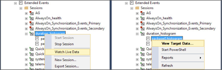
Figure 13-2 A side-by-side look at the difference between Watch Live Data on an extended events session and View Target Data on an extended events session target.
When viewing target data, you can right-click to re-sort, copy the data to clipboard, and export most of the target data to .csv files for analysis in other software.
Unlike Watch Live Data, View Target Data does not refresh automatically, though for some targets, you can configure SQL Server Management Studio to poll the target automatically by right-clicking the View Target Data window and then clicking Refresh Interval.
The section that follows presents a breakdown of the possible targets, many of which do some of the serious heavy lifting that you might have done previously by writing or exporting SQL trace data to a table and then performing your own aggregations and queries. Remember that you don’t need to pick just one target type to collect data for your session, but that a target can’t collect data prior to its creation.
Understanding the variety of extended events targets
Here is a summary of the extended event targets available to be created. Remember you can create more than one target per Session.
Event File target (.xel), which writes the event data to a physical file on a drive, asynchronously. You can then open and analyze it later, much like deprecated trace files, or merge it with other .xel files to assist analysis (in SQL Server Management Studio, click the File menu, click Open, and then click Merge Extended Events Files).
However, when you view the event file data in SQL Server Management Studio by right-clicking the event file and selecting View Target Data, the data does not refresh live. Data continues to be written to the file behind the scenes while the session is running, so to view the latest data, close the .xel file and open it again.
Histogram, which counts the number of times an event has occurred and bucketizes an action, storing the data in memory. For example, you could capture a histogram of the
sql_statement_completedbroken down by the number of observed events by client-hostname action, or by the duration field.Be sure to provide a number of buckets (or slots, in the T-SQL syntax) that is greater than the number of unique values you expect for the action or field. If you’re bucketizing by a numeric value such as duration, be sure to provide a number of buckets larger than the largest duration you could capture over time. If the histogram runs out of buckets for new values for your action or field, it will not capture data for them!
Note that you can provide any number of histogram buckets, but the histogram target will round the number up to the nearest power of 2. Thus, if you provide a value of 10 buckets, you’ll see 16 buckets.
Pair matching, which is used to match events, such as the start and end of a SQL Server batch execution, and find occasions when an event in a pair occurs without the other, such as
sql_statement_startingandsql_statement_completed. Select a start and an end from the list of actions you’ve selected.Ring_bufferprovides a fast, in-memory First-In, First-Out (FIFO) asynchronous memory buffer to collect rapidly occurring events. Stored in a memory buffer, the data is never written to a drive, allowing for robust data collection without performance overhead. The customizable dataset is provided in XML format and must be queried. Because this data is in-memory, you should be careful how high you configure the Maximum Buffer Memory size, and never set the size to 0 (unlimited).Finally, you can use the Service Broker target to send messages to a target service of a customizable message type.
Although all of the aforementioned targets are high-performing asynchronous targets, there are a pair of synchronous targets: ETW and event counter. Be aware when using synchronous targets that the resource demand of synchronous targets might be more noticeable. Following is a brief description of each asynchronous target:
ETW (Event Tracing for Windows). This is used to gather SQL Server data for later combination to Windows event log data for troubleshooting and debugging Windows applications.
Event counter. This simply counts the number of events in an extended events session. You use this to provide data for trending and later aggregate analysis. The resulting dataset has one row per event with a count. This data is stored in memory, so although it’s synchronous, you shouldn’t expect any noticeable performance impact.
Let’s look at querying extended events session data in T-SQL with a couple of practical common examples.
Using extended events to detect deadlocks
We’ve talked about viewing data in SQL Server Management Studio, so let’s review querying extended events data via T-SQL. Let’s query one of the default extended events sessions, system_health, for deadlocks. Back in the dark ages, before SQL Server 2008, it was not possible to see a deadlock. You had to see it coming—to turn on a trace flag prior to the deadlock.
With the system_health extended events session, a recent history (a rolling 4-MB buffer) of event data in the ring_buffer target will contain any occurrences of the xml_deadlock_report event.
The T-SQL code sample that follows demonstrates the retrieval of the ring_buffer target as XML, and the use of XQuery syntax:
WITH cteDeadlocks ([Deadlock_XML]) AS (
--Query RingBufferTarget
SELECT [Deadlock_XML] = CAST(target_data AS XML)
FROM sys.dm_xe_sessions AS xs
INNER JOIN sys.dm_xe_session_targets AS xst
ON xs.address = xst.event_session_address
WHERE xs.NAME = 'system_health'
AND xst.target_name = 'ring_buffer'
)
SELECT
Deadlock_XML = x.Graph.query('(event/data/value/deadlock)[1]') --View as XML for
detail, save this output as .xdl and re-open in SSMS for visual graph
, Deadlock_When = x.Graph.value('(event/data/value/deadlock/process-list/process/@last-
batchstarted)[1]', 'datetime2(3)') --date the last batch in the first process started,
only an approximation of time of deadlock
, DB = DB_Name(x.Graph.value('(event/data/value/deadlock/process-list/process/@cur-
rentdb)[1]', 'int')) --Current database of the first listed process
FROM (
SELECT Graph.query('.') AS Graph
FROM cteDeadLocks c
CROSS APPLY c.[Deadlock_XML].nodes('RingBufferTarget/event[@name="xml_deadlock_
report"]') AS Deadlock_Report(Graph)
) AS x
ORDER BY Deadlock_When desc;
This example returns one row per captured xml_deadlock_report event and includes an XML document, which in SQL Server Management Studio Grid results will appear to be a blue hyperlink. Click the hyperlink to open the XML document, which will contain the complete detail of all elements of the deadlock. If you’d like to see a Deadlock Graph, save this file as an .xdl file, and then open it in SQL Server Management Studio.
You can download the previous script, CH12_XEvents.sql, and other accompanying sample scripts for this book from https://aka.ms/SQLServ2017Admin/downloads.
Using extended events to detect autogrowth events
The SQL Server default trace captures historical database data and log file autogrowth events, but the default extended events sessions shipped with SQL Server do not. The extended events that capture autogrowth events are database_file_size_change and databases_log_file_size_changed. Both events capture autogrowths and manual file growths run by ALTER DATABASE … MODIFY FILE statements, and include an event field called is_automatic to differentiate. Additionally, you can identify the query statement sql_text that prompted the autogrowth event.
Following is a sample T-SQL script to create a startup session that captures autogrowth events to an .xel event file and also a histogram target that counts the number of autogrowth instances per database:
CREATE EVENT SESSION [autogrowths] ON SERVER
ADD EVENT sqlserver.database_file_size_change(
ACTION(package0.collect_system_time,sqlserver.database_id
,sqlserver.database_name,sqlserver.sql_text)),
ADD EVENT sqlserver.databases_log_file_size_changed(
ACTION(package0.collect_system_time,sqlserver.database_id
,sqlserver.database_name,sqlserver.sql_text))
ADD TARGET package0.event_file(
--.xel file target
SET filename=N'F:DATAautogrowths.xel'),
ADD TARGET package0.histogram(
--Histogram target, counting events per database_name
SET filtering_event_name=N'sqlserver.database_file_size_change'
,source=N'database_name',source_type=(0))
--Start session at server startup
WITH (STARTUP_STATE=ON);
GO
--Start the session now
ALTER EVENT SESSION [autogrowths]
ON SERVER STATE = START;
Using extended events to detect page splits
As we discussed earlier in this chapter, detecting page splits can be useful. You might choose to monitor page_splits when load testing a table design with its intended workload or when finding insert statements that cause the most fragmentation.
The following sample T-SQL script creates a startup session that captures autogrowth events to an .xel event file and also a histogram target that counts the number of page_splits per database:
CREATE EVENT SESSION [page_splits] ON SERVER
ADD EVENT sqlserver.page_split(
ACTION(sqlserver.database_name,sqlserver.sql_text))
ADD TARGET package0.event_file(
SET filename=N'page_splits',max_file_size=(100)),
ADD TARGET package0.histogram(
SET filtering_event_name=N'sqlserver.page_split'
,source=N'database_id',source_type=(0))
--Start session at server startup
WITH (STARTUP_STATE=ON);
GO
--Start the session now
ALTER EVENT SESSION [page_splits]
ON SERVER STATE = START;
Securing extended events
To access extended events, a developer or analyst needs the ALTER ANY EVERY SESSION permission. This is different from the ALTER TRACE permission needed for traces. This grants that person access to create extended events sessions by using T-SQL commands, but it will not grant access to view server metadata in the New Extended Events Session Wizard in SQL Server Management Studio. For that, the person needs one further commonly granted developer permission, VIEW SERVER STATE. In Azure SQL Database, extended events have the same capability, but for developers to view extended events sessions, you must grant them an ownership-level permission CONTROL DATABASE. However, we do not recommend this for developers or non-administrators in production environments.
There are certain sensitive events that you cannot capture with a trace or extended event session; for example, the T-SQL statement CREATE LOGIN for a SQL-authenticated login.
Capturing Windows performance metrics with DMVs and data collectors
The Performance Monitor (perfmon.exe) application has been used for years by server administrators to visually track and collect performance of server resources, application memory usage, disk response times, and so on. In addition to the live Performance Monitor graph, you can also configure Data Collector Sets to gather the same Performance Monitor metrics over time.
SQL Server has a large number of metrics captured within, as well. Although we have neither the scope nor space to investigate and explain each one in this book, here is a sampling of some performance metrics you might find valuable when reviewing the health and performance of your SQL Server.
These metrics are at the Windows server level or SQL Server instance level, so it is not possible to get granular data for individual databases, workloads, or queries; however, identifying performance with isolated workloads in near-production systems is possible. Like aggregate wait statistics, there is significant value in trending these Performance Monitor metrics on server workloads, monitoring peak behavior metrics, and for immediate troubleshooting and problem diagnosis.
Querying performance metrics by using DMVs
Beyond Performance Monitor, we’ve already seen in this chapter a DMV that exposes most of the performance metrics within SQL Server, sys.dm_os_performance_counters. There are some advantages to this DMV in that you can combine it with other DMVs that report on system resource activity (check out sys.dm_os_sys_info, for example), and you can fine-tune the query for ease of monitoring and custom data collecting. However, sys.dm_os_performance_counters does not currently have access to metrics outside of the SQL Server instance categories, even the most basic Windows metrics such as “% Processor Time.”
This following straightforward code sample uses sys.dm_os_performance_counters to return the instance’s current target server memory, total server memory, and page life expectancy:
SELECT InstanceName = @@SERVERNAME
, Target_Server_Mem_GB = max(CASE counter_name
WHEN 'Target Server Memory (KB)' THEN convert(decimal(19,3), cntr_value/1024./1024.)
END)
, Total_Server_Mem_GB = max(CASE counter_name
WHEN 'Total Server Memory (KB)' THEN convert(decimal(19,3), cntr_value/1024./1024.)
END)
, PLE_s = MAX(CASE counter_name WHEN 'Page life expectancy' THEN cntr_value END)
FROM sys.dm_os_performance_counters;;
Some queries against sys.dm_os_performance_counters are not as straightforward. As an example, although Performance Monitor returns Buffer Cache Hit Ratio as a single value, querying this same memory metric via the DMV requires creating the ratio from two metrics. This code sample divides two metrics to provide the Buffer Cache Hit Ratio:
SELECT Buffer_Cache_Hit_Ratio = 100 *
(SELECT cntr_value = convert(decimal (9,1), cntr_value)
FROM sys.dm_os_performance_counters as pc
WHERE pc.COUNTER_NAME = 'Buffer cache hit ratio'
AND pc.OBJECT_NAME like '%:Buffer Manager%')
/
(SELECT cntr_value = convert(decimal (9,1), cntr_value)
FROM sys.dm_os_performance_counters as pc
WHERE pc.COUNTER_NAME = 'Buffer cache hit ratio base'
AND pc.OBJECT_NAME like '%:Buffer Manager%');
Finally, some counters returned by sys.dm_os_performance_counts are continually incrementing integers. Let’s return to our example of finding page splits. The counter_name “Page Splits/sec” is misleading when accessed via the DMV, but it is in fact an incrementing number. To calculate the rate of page splits per second, we need two samples. This strategy is appropriate only for single-value counters for the entire server or instance. For counters that return one value per database, you would need a temp table in order to calculate the rate for each database between the two samples.
DECLARE @page_splits_Start_ms bigint, @page_splits_Start bigint
, @page_splits_End_ms bigint, @page_splits_End bigint
SELECT @page_splits_Start_ms = ms_ticks
, @page_splits_Start = cntr_value
FROM sys.dm_os_sys_info
CROSS APPLY sys.dm_os_performance_counters
WHERE counter_name ='Page Splits/sec'
AND object_name LIKE '%SQL%Access Methods%'
WAITFOR DELAY '00:00:10' --Adjust sample duration between measurements, 10s sample
SELECT @page_splits_End_ms = MAX(ms_ticks), @page_splits_End = MAX(cntr_value)
FROM sys.dm_os_sys_info
CROSS APPLY sys.dm_os_performance_counters
WHERE counter_name ='Page Splits/sec'
AND object_name LIKE '%SQL%Access Methods%'
SELECT Page_Splits_per_s = (@page_splits_End - @page_splits_Start)*1.
/ NULLIF(@page_splits_End_ms - @page_splits_Start_ms,0)*1.;
However, you can gain access to some Windows metrics via the DMV sys.dm_os_ring_buffers, including metrics on CPU utilization and memory. This internal DMV returns thousands of XML documents, generated every second, loaded with information on SQL exceptions, memory, schedulers, connectivity, and more.
In the code sample that follows, we pull the SQL Server instance’s current CPU utilization percentage and the current server idle CPU percentage. The remaining CPU percentage can be chalked up to other applications or services running on the Windows server, including other SQL Server instances.
SELECT
[Time] = DATEADD(ms, -1 * (si.cpu_ticks
/ (si.cpu_ticks/si.ms_ticks) - x.[timestamp])
, SYSDATETIMEOFFSET ())
, CPU_SQL_pct = bufferxml.value('(./Record/SchedulerMonitorEvent
/SystemHealth/ProcessUtilization)[1]', 'int')
, CPU_Idle_pct = bufferxml.value('(./Record/SchedulerMonitorEvent
/SystemHealth/SystemIdle)[1]', 'int')
FROM (SELECT timestamp, CONVERT(xml, record) AS bufferxml
FROM sys.dm_os_ring_buffers
WHERE ring_buffer_type = N'RING_BUFFER_SCHEDULER_MONITOR') AS x
CROSS APPLY sys.dm_os_sys_info AS si
ORDER BY [Time] desc;
The built-in SQL Server ring_buffer data collector isn’t Performance Monitor and doesn’t resemble it at all, though it does provide data at certain events. In the case of CPU utilization in the Scheduler_Monitor ring buffer, we get fresh data once per second. Other data streams aren’t as constant. In the case of SQL Server memory utilization, for example, we can get snapshots of key memory metrics only when one of four memory events are initiated: high or low physical memory, low virtual memory, or a steady event that indicates that the previous memory pressure event has been relieved. The frequency of these memory events is inconsistent and might not happen for weeks at a time, but could still be valuable for troubleshooting memory conditions on the SQL Server. Let’s look at the code:
SELECT
[Time] = DATEADD(ms, -1 * (si.cpu_ticks
/ (si.cpu_ticks/si.ms_ticks) - x.[timestamp])
, SYSDATETIMEOFFSET ())
, MemoryEvent = bufferxml.value('(./Record/ResourceMonitor
/Notification)[1]', 'varchar(64)')
, Target_Server_Mem_GB = CONVERT (decimal(19,3),
bufferxml.value('(./Record/MemoryNode/TargetMemory)[1]'
, 'bigint')/1024./1024.)
, Physical_Server_Mem_GB = CONVERT (decimal(19,3),
bufferxml.value('(./Record/MemoryRecord/TotalPhysicalMemory)[1]'
, 'bigint')/1024./1024.)
, Committed_Mem_GB = CONVERT (decimal(19,3),
bufferxml.value('(./Record/MemoryNode/CommittedMemory)[1]'
, 'bigint')/1024./1024.)
, Shared_Mem_GB = CONVERT (decimal(19,3),
bufferxml.value('(./Record/MemoryNode/SharedMemory)[1]'
, 'bigint')/1024./1024.)
, MemoryUtilization = bufferxml.value('(./Record/MemoryRecord
/MemoryUtilization)[1]', 'bigint')
, Available_Server_Mem_GB = CONVERT (decimal(19,3), bufferxml.value('(./Record/MemoryRe-
cord/AvailablePhysicalMemory)[1]'
, 'bigint')/1024./1024.)
FROM (SELECT timestamp, CONVERT(xml, record) AS bufferxml
FROM sys.dm_os_ring_buffers
WHERE ring_buffer_type = N'RING_BUFFER_RESOURCE_MONITOR') AS x
CROSS APPLY sys.dm_os_sys_info AS si
ORDER BY [Time] desc;
Querying performance metrics by using Performance Monitor
To get a complete and graphical picture of server resource utilization, using a server resource tool is necessary. Performance Monitor is more than just a pretty graph, it is a suite of data collection tools that can persist outside of your user profile.
You can configure the live Performance Monitor graph, available in the Monitoring Tools folder, to show a live picture of server performance. To do so, right-click the (mostly empty) grid to access properties, add counters, clear the graph, and so on. In the Properties dialog box, under General, you can configure the sample rate and duration of the graph. You can display up to 1,000 sample points on the graph live. This can be 1,000 one-second sample points for a total of 16 minutes and 40 seconds, or more time if you continue to decrease the sample frequency. For example, you can display 5,000 five-second sample points for more than 83 minutes of duration in the graph.
To view data collected by Data Collectors, stop the data collector and restart it. In the Reports folder, in the User Defined folder, you’ll see a new report that contains the graph that the Data Collector created. Figure 13-3 shows that more than 15 days of data performance was collected in the Data Collector, which we’re viewing in the Memory folder, selecting the most recent report that was generated when we stopped the Memory Data Collector Set.

Figure 13-3 The Windows Performance Monitor Application. Instead of showing live data from the Monitoring Tools-Performance Monitor screen, we’re showing 15 days’ worth of data recorded by a User Defined Data Collector Set, which generated a User Defined Report.
Monitoring key performance metrics
Here are some Performance Monitor metrics to take a look at when gauging the health and performance of your SQL Server. Although we don’t have the space in this book to provide a deep dive into each metric, its causes, and indicators, you should take time to investigate and research metrics that appear out of line with the guidelines provided here.
We don’t provide many hard numbers in this section; for example, “Metrix X should always be lower than Y.” You should trend, measure metrics at peak activity, and investigate how metrics respond to server, query, or configuration changes. What might be normal for an instance with a read-heavy workload might be problematic for an instance with a high-volume write workload, and vice versa.
We do explain how to find the metric in both Performance Monitor’s Add Counters menu and the DMV sys.dm_os_performance_counters, when available.
Average Disk seconds per Read or Write
Performance Monitor: PhysicalDisk:Avg. Disk sec/Read and PhysicalDisk:Avg. Disk sec/Write
DMV: Not Available
View this metric on each volume. The “_Total” metric doesn’t have any value here, you should look at individual volumes in which SQL Server files are present. This metric has the clearest guidance of any with respect to what is acceptable or not for a server. Try to measure this value during your busiest workload and also during backups. You want to see the average disk seconds per read and write operation (considering that a single query could have thousands or millions of operations) below 20 ms, or .02 seconds. Below 10 ms is optimal and very achievable with modern storage systems. (This is the rare case for which we actually have hard and fast numbers specified by Microsoft to rely on.) Seeing this value spike to very high values (such as .1 second or 100 ms) isn’t a major cause for concern, but if you see these metrics sustaining an average higher than .02 seconds during peak activity, this is a fairly clear indication that the physical I/O subsystem is being stressed beyond its capacity to keep up. Low, healthy measurements for this number don’t provide any insight into the quality of or efficiency of queries and execution plans, only the response from the disk subsystem. The Avg. Disk sec/Transfer counter is simply a combination of both read and write activity, unrelated to Avg. Disk Transfers/sec. (Confusing, we know!)
Page Life Expectancy (PLE)
Performance Monitor: MSSQL$Instance:Buffer Manager/Page Life Expectancy (s)
DMV: MSSQL$Instance:Buffer Manager/Page life expectancy
PLE is a measure of time that indicates the age of data in memory. In general, you want pages of data in memory to grow to a ripe old age—it means that there is ample memory available to SQL Server to store data to serve reads without going back to a drive. A dated metric of 300 seconds might only be appropriate for servers with less than 64 GB of memory. With more and more memory available to a SQL instance, the older the average data page should be as data remains cached longer, so 300 seconds could be appropriate for a server with 4 GB of memory, but far too low for a server with 64 GB of memory. PLE is one of the most direct indicators of memory pressure, though it doesn’t provide a complete picture of memory utilization in SQL Server.
Buffer Cache Hit Ratio (BCHR)
Performance Monitor: MSSQL$Instance:Buffer Manager/Buffer Cache Hit Ratio
DMV: MSSQL$Instance:Buffer Manager/Buffer cache hit ratio divided by MSSQL$Instance:Buffer Manager/Buffer cache hit ratio base
A value from 0 to 100, where 100 means that recent traffic has been served entirely out of buffer cache, and 0 means data has been served from a drive. This is not a complete picture of memory pressure, and good high values (>90%) shouldn’t be a definitive indication that there is no memory pressure. Low values do indicate a clear indicator that memory is not sufficient for the current workload, but this can also be misleading. Backups and index maintenance can cause BCHR to drop precipitously, to values near zero. Although this metric should be a part of your puzzle, values greater than 80% are desirable.
Page Reads
Performance Monitor: MSSQL$Instance:Buffer Manager/Page reads/sec
DMV: MSSQL$Instance:Buffer Manager/Page reads/sec
The title is a bit misleading—these aren’t page reads out of the buffer; rather, they are out of physical pages on the drive, which is slower than data pages coming out of memory. You should make the effort to lower this number by optimizing queries and indexing, efficiency of cache storage, and, of course, as a last resort, increasing the amount of server memory. Although every workload is different, a value less than 90 is a broad guideline. High numbers indicate inefficient query and index design in read-write workloads, or memory constraints in read-heavy workloads.
Memory Pages
Performance Monitor: Memory:Pages/sec
DMV: Not available
Similar to Buffer ManagerPage Reads/sec, this is a way to measure data coming from a drive as opposed to coming out of memory. It is a measure of pages pulled from a drive into memory, which will be high after SQL Server startup. Although every workload is different, a value less than 50 is a broad guideline. Sustained high or climbing levels during typical production usage indicate inefficient query and index design in read-write workloads, or memory constraints in read-heavy workloads. Spikes during database backup and restore operations, bulk copies, and data extracts are expected.
Batch Requests
Performance Monitor: MSSQL$lnstance:SQL StatisticsBatch Requests/sec
DMV: MSSQL$lnstance:SQL StatisticsBatch Requests/sec
A measure of aggregate SQL Server user activity. Higher sustained numbers are good; they mean your SQL instance is sustaining more traffic. Should this number trend downward during peak business hours, your SQL Server instance is being outstripped by increasing user activity.
Page Faults
Performance Monitor: MemoryPage Faults/sec
DMV: Not Available
A memory page fault occurs when an application seeks a data page in memory, only to find it isn’t there because of memory churn. A soft page fault indicates the page was moved or otherwise unavailable; a hard page fault indicates the data page was not in memory and must be retrieved from the drive. The Page Faults/sec metric captures both. Page faults are a symptom, the cause being memory churn, so you might see an accompanying drop in the Page Life Expectancy. Spikes in Page Faults, or an upward trend, indicate the amount of server memory was insufficient to serve requests from all applications, not just SQL Server.
Available Memory
Performance Monitor: MemoryAvailable Bytes or MemoryAvailable KBytes or MemoryAvailable MBytes
DMV: Available in sys.dm_os_ring_buffers WHERE ring_buffer_type = RING_BUFFER_RESOURCE_MONITOR (see previous section)
Available Memory is server memory currently unallocated to an application. Server memory above and beyond what the SQL Server instance(s) total MAX_SERVER_MEMORY setting, minus memory in use by other SQL Server features and services or other applications, are available. This will roughly match what shows as available memory in the Windows Task Manager.
Total Server Memory
Performance Monitor: MSSQL$Instance:Memory ManagerTotal Server Memory (KB)
DMV: MSSQL$Instance:Memory ManagerTotal Server Memory (KB)
This is the actual amount of memory that SQL Server is using. It is often contrasted with the next metric (Target Server Memory). This number might be far larger than what Windows Task Manager shows allocated to the SQL Server Windows NT – 64 Bit background application, which shows only a portion of the memory that sqlserver.exe controls. The Total Server Memory metric is correct.
Target Server Memory
Performance Monitor: MSSQL$Instance:Memory ManagerTarget Server Memory (KB)
DMV: MSSQL$Instance:Memory ManagerTarget Server Memory (KB)
This is amount of memory to which SQL Server wants to have access and is currently working toward consuming. If the difference between Target Server Memory and Total Server Memory is larger than the value for Available Memory, SQL Server wants more memory than the Windows Server can currently acquire. SQL Server will eventually consume all memory available to it under the MAX_SERVER_MEMORY setting, but it might take time.
Protecting important workloads by using Resource Governor
Resource Governor is an Enterprise edition–only feature that you can use to identify connections and limit the resources they can consume.
You can identify connections from virtually any connection property, including the login name, hostname, application name, and so on. After you’ve identified them, you can limit properties at the individual session level or in a pool of resources. You can override the MAXDOP setting for these sessions; or lower their priority; or cap the CPU, memory, or drive I/O that individual sessions can consume.
For example, you can limit all read-heavy queries coming from a SQL Server Reporting Services server, or long-running reports coming from a third-party reporting application, or dashboard/search queries that use a different application name or login. Then, you can limit these queries as a set, capping them to 25% of the process, disk I/O, or SQL Server memory. SQL Server will enforce these limitations and potentially slow down the identified queries, but meanwhile, the important read-write workloads continue to operate with the remaining 75% of the server’s resources.
Be aware that using Resource Governor to limit long-running SELECT statements, for example, does not alleviate concurrency issues caused by locking. See Chapter 9 for strategies to overcome concurrency issues, and keep in mind that using the NOLOCK table hint or the READ UNCOMMITTED isolation level is a risky, clumsy strategy to solving concurrency issues in your applications.
When turned on, Resource Governor is transparent to connecting applications. No code changes are required of the queries to implement Resource Governor.
In Enterprise edition, by default, sessions are split between group = 1 named “system,” for system queries internal to the Database Engine, and group = 2 named “default,” for all user other user queries. In Standard edition of SQL Server, Resource Governor is not provided, and the only value for group_id is 1. You can find the current groups in the DMV sys.resource_governor_workload_groups.
Configuring the Resource Governor classifier function
Before turning on Resource Governor, you must create a classifier function in the master database that operates at the creation of every new session.
You can write the classifier function however you like, but keep in mind that it will be run for each new connection, and so it should be as efficient and simple as possible. Do not query other user resources such as tables in a user database, because this can cause a noticeable delay in connection creation.
The classifier function must return a Sysname datatype value, which contains the name of the Group to which a new connection is to be assigned. A Group is simply a container of sessions. If no Group name is assigned, the connection is placed in the default group. Remember, it is the default group that you want to protect; it contains “all other” sessions including high business-value connections that perform application-critical functions, writes, and so on.
The sample code that follows defines a classifier function that returns GovGroupReports for all queries coming from two known-fictional reporting servers. You can see in the comments other sample connection identifying functions, with many more options possible.
CREATE FUNCTION dbo.fnCLASSIFIER() RETURNS sysname
WITH SCHEMABINDING AS
BEGIN
-- Note that any request that does not get classified goes into the 'default' group.
DECLARE @grp_name sysname
IF (
--Use built-in functions for connection string properties
HOST_NAME() IN ('reportserver1','reportserver2')
--OR APP_NAME() IN ('some application')
--AND SUSER_SNAME() IN ('whateveruser')
)
BEGIN
SET @grp_name = 'GovGroupReports';
END
RETURN @grp_name
END;
After creating the function, you must register it (which can have any name) as the classifier function for this instance’s Resource Governor feature. The feature is not active yet; you still have the following setup to do before turning it on:
-- Register the classifier function with Resource Governor
ALTER RESOURCE GOVERNOR WITH (CLASSIFIER_FUNCTION= dbo.fnCLASSIFIER);
Configuring Resource Governor pools and groups
Configuring pools (for many sessions to share) and groups (for individual sessions) is the next step. You should take an iterative, gradual approach to configuring the Governor, and avoid making large changes or large initial limitations to the affected groups.
If you have a Developer edition preproduction environment to test the impact of Resource Governor on workloads with realistic production scale, you should consider testing.
The sample code that follows can be an instructional template to creating an initial Pool and Group. If you seek to divide your sessions up further, multiple groups can belong to the same pool, and multiple pools can be limited differently. Commented-out examples of other common uses for Resource Governor are included.
In this example, we create a pool that limits all covered sessions to 50% of the instance’s memory, and a group that limits any single query to 30% of the instance’s memory, and forces the sessions into MAXDOP = 1, overriding any server, database, or query-level setting:
CREATE RESOURCE POOL GovPoolMAXDOP1;
CREATE WORKLOAD GROUP GovGroupReports;
GO
ALTER RESOURCE POOL GovPoolMAXDOP1
WITH (-- MIN_CPU_PERCENT = value
--,MAX_CPU_PERCENT = value
--,MIN_MEMORY_PERCENT = value
MAX_MEMORY_PERCENT = 50
);
GO
ALTER WORKLOAD GROUP GovGroupReports
WITH (
--IMPORTANCE = { LOW | MEDIUM | HIGH }
--,REQUEST_MAX_CPU_TIME_SEC = value
--,REQUEST_MEMORY_GRANT_TIMEOUT_SEC = value
--,GROUP_MAX_REQUESTS = value
REQUEST_MAX_MEMORY_GRANT_PERCENT = 30
, MAX_DOP = 1
)
USING GovPoolMAXDOP1;
![]() For complete documentation of the possible ways to limit groups and pools, go to https://docs.microsoft.com/sql/t-sql/statements/alter-workload-group-transact-sql and https://docs.microsoft.com/sql/t-sql/statements/alter-resource-pool-transact-sql
For complete documentation of the possible ways to limit groups and pools, go to https://docs.microsoft.com/sql/t-sql/statements/alter-workload-group-transact-sql and https://docs.microsoft.com/sql/t-sql/statements/alter-resource-pool-transact-sql
After you have configured the classifier function, groups, and pools, you can turn on Resource Governor by using the query that follows, placing its functionality into memory. New sessions will begin being sorted by the classifier function and new sessions will appear in their groups. You should also issue the reconfigure command to apply changes made:
-- Start or Reconfigure Resource Governor
ALTER RESOURCE GOVERNOR RECONFIGURE;
Or, you can turn it off:
--Disable Resource Governor
ALTER RESOURCE GOVERNOR DISABLE;
After you turn it off, existing sessions will continue to operate under the rules of Resource Governor, but new queries will not be sorted into groups.
After you configure it and turn it on, you can query the status of Resource Governor and the name of the classifier function by using the following sample script:
SELECT rgc.is_enabled, o.name
FROM sys.resource_governor_configuration AS rgc
INNER JOIN master.sys.objects AS o
ON rgc.classifier_function_id = o.object_id
INNER JOIN master.sys.schemas AS s
ON o.schema_id = s.schema_id;
Monitoring pools and groups
The Group_ID columns in both sys.dm_exec_requests and sys.dm_exec_sessions define to which Resource Governor Group the request or session is a part. Groups are members of pools. You can query the groups and pools via the DMVs sys.resource_governor_workload_groups and sys.resource_governor_resource_pools. Use the following sample query to observe the number of sessions that have been sorted into groups, noting that group_id = 1 is the internal group, group_id = 2 is the default group, and other groups defined by you, the administrator:
SELECT
rgg.group_id, rgp.pool_id
, Pool_Name = rgp.name, Group_Name = rgg.name
, session_count= ISNULL(count(s.session_id) ,0)
FROM sys.dm_resource_governor_workload_groups AS rgg
LEFT OUTER JOIN sys.dm_resource_governor_resource_pools AS rgp
ON rgg.pool_id = rgp.pool_id
LEFT OUTER JOIN sys.dm_exec_sessions AS s
ON s.group_id = rgg.group_id
GROUP BY rgg.group_id, rgp.pool_id, rgg.name, rgp.name
ORDER BY rgg.name, rgp.name;
![]() You can reference a (dated) Resource Governor troubleshooting guide for a list of error numbers and their meanings that might be raised by Resource Governor at https://technet.microsoft.com/library/cc627395%28v=sql.105%29.aspx.
You can reference a (dated) Resource Governor troubleshooting guide for a list of error numbers and their meanings that might be raised by Resource Governor at https://technet.microsoft.com/library/cc627395%28v=sql.105%29.aspx.
Understanding the new servicing model
Database administrators and CIOs alike will need to adjust their normal comfort levels with new SQL Server editions. No longer can IT leadership say, “Wait until the first service pack,” before moving because there are no more service packs!
Updated servicing model
Microsoft has adopted a new model for its product life cycles. In the past, this servicing model included Service Packs (SPs), Cumulative Updates (CUs), and General Distribution Releases (GDRs). Beginning with SQL Server 2017, the following changes are in effect:
SPs will no longer be released.
CUs will be released every month for the first twelve months of general release, and then quarterly for the remaining four years of the five-year duration of the Mainstream Support period.
CUs might now include localized content and will be delivered on a standardized schedule: as of this writing, this is the week of the third Tuesday of the month.
Unlike in the past, GDR patches (which contain security-only fixes) will not have their own path for updates between CUs.
Microsoft has maintained in recent years that there is no need to wait for an SP, because the General Availability (GA) release has been extensively tested by both internal Microsoft QA and external preview customers. In fact, Microsoft insists that the Community Technology Preview (CTP) and Release Candidate (RC) versions of SQL Server 2016 and 2017, the steps before Release to Market (RTM), were thoroughly tested in production with selected customers. For those dealing with clients or leadership who are stubborn or reactionary, a possible alternative under the new model could be to target an arbitrary Cumulative Update, such as CU2.
Product support life cycle
In you’re planning for long-term use of a particular version of SQL Server, you should keep in mind the following life cycle:
0 to 5 Years: Mainstream Support Period
Security and functional issues are addressed through CUs. Security issues only might also be addressed through GDRs.
6 to 10 Years: Extended Support
Only critical functional issues will be addressed. Security issues might still be addressed through GDRs
11 to 16 Years: Premium Assurance
The Extended Support level can be lengthened with optional payments.