
1 Set up a workbook
In this chapter
Practice files
For this chapter, use the practice files from the Excel2019SBSCh01 folder. For practice file download instructions, see the introduction.
When you create a new Excel 2019 workbook, the app presents a blank workbook that contains one worksheet. You can add or delete worksheets, hide worksheets within the workbook without deleting them, and change the order of your worksheets within the workbook. You can also copy a worksheet to another workbook or move the worksheet without leaving a copy of the worksheet in the first workbook. If you and your colleagues work with a large number of documents, you can define property values to make your workbooks easier to find when you and your colleagues attempt to locate them by using the Windows search box.
Another way to make Excel easier to use is by customizing the Excel app window to fit your work style. If you find that you use a command frequently, you can add it to the Quick Access Toolbar so it’s never more than one click away. If you use a set of commands frequently, you can create a custom ribbon tab, so they appear in one place. You can also hide, display, or change the order of the tabs on the ribbon.
This chapter guides you through procedures related to creating and modifying workbooks, creating and modifying worksheets, merging and unmerging cells, and customizing the Excel 2019 app window. First, however, it introduces you to the various editions of Excel 2019, and new features of the software.
Explore the editions of Excel 2019
The Microsoft Office 2019 suite includes apps that give you the ability to create and manage every type of file you need to work effectively at home, work, or school. The apps include Microsoft Word, Excel, Outlook, PowerPoint, Access, OneNote, and Publisher. You can purchase the apps as part of a package that includes multiple apps or purchase most of the apps individually.
Using the Office 2019 apps, you can find the tools you need quickly. Moreover, because they were designed as an integrated package, you’ll find that the skills you learn in one app transfer readily to the others. That flexibility extends well beyond your personal computer. In addition to the traditional desktop edition of Excel, you can also use Excel Online in combination with Microsoft OneDrive (formerly called SkyDrive).
Excel 2019
The click-to-run version of Excel 2019 is installed directly on your computer. The desktop version of the app includes all the capabilities built into Excel 2019. You can purchase Excel 2019 as part of an Office app suite or as a separate app.
![]() Tip
Tip
Office 365 is a cloud-based subscription licensing solution that provides access to a continually updated version of Excel, which adds new capabilities on a regular basis. Excel 2019 receives security updates but not feature updates.
Excel Online
Information workers require their data to be available to them at all times, not just when they’re using their personal computers. To provide mobile workers with access to their data, Microsoft developed Office Online, which includes online versions of Excel, Word, PowerPoint, Outlook, and OneNote. Office Online is available as part of an Office 365 subscription or for free as part of the OneDrive cloud service.
You can use Excel Online to edit files stored in your OneDrive account or on a Microsoft SharePoint site. Excel Online displays your Excel files (version 2010 and later) as they appear in the desktop version of the app and includes all the functions you use to summarize your data. You can also view and manipulate PivotTables, add charts, and format your data to communicate its meaning clearly.
You can also use Excel Online to share your workbooks online, embed them as part of another webpage, and create web-accessible surveys that save user responses directly to an Excel workbook in your OneDrive account.
After you open a file by using Excel Online, you can choose to continue editing the file in your browser or open the file in the desktop app. When you open the file in your desktop app, any changes you save are written to the version of the file on your OneDrive account. This means that you will always have access to the most recent version of your file, regardless of where and how you access it.
At the time of this writing, Excel Online is compatible with the most recent versions of Microsoft Edge, Internet Explorer 11 and later, Mozilla Firefox, and Google Chrome for Windows. You can also use Excel Online on a Mac if you have the most recent version of Safari or Chrome, as well as on Linux with Firefox or Chrome, although some features might not be available. Most Office Online features are also supported in Microsoft Edge for HoloLens and Xbox One.
You can use Excel Online on Apple devices running iOS versions earlier than 10.0. For iOS 10.0 or later, it’s recommended that you use the Office for iPad or Office for iPhone app. There are no officially supported Android browsers for Office Online, but you can use the Office for Android apps instead.
Excel Mobile Apps
Office for iPad and Office for iPhone require iOS 10.0 or later. If you own an Android device, Office for Android can be installed on tablets and phones that are running Android KitKat 4.4 or later and that have an ARM-based or Intel x86 processor.
Become familiar with new features in Excel 2019
Excel 2019 includes all the most useful capabilities included in previous versions of the app. If you’ve used an earlier version of Excel, you probably want to know about the new features introduced in Excel 2019. These include the following:
Funnel charts and 2D maps, which let users visualize data more effectively
New worksheet functions and data connectors for importing and summarizing data
The capability to publish Excel data to Power BI, the data visualization and dashboarding app from Microsoft
Enhancements to PowerPivot and Power Query, which enable users to import, process, and summarize millions of rows of data
Create workbooks
Any time you want to gather and store data that isn’t closely related to any of your other existing data, you should create a new workbook. A workbook is the basic Excel file, comparable to a Microsoft Word document or Microsoft PowerPoint presentation. The default new workbook in Excel has one worksheet, which is like a page in a Word document or a slide in a PowerPoint presentation. You can add more worksheets to help organize your data more effectively. When you start Excel, the app displays the Start screen.
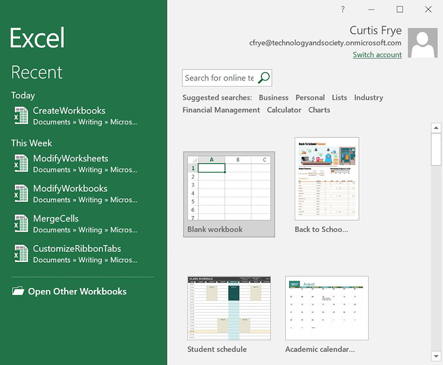
The Start screen is part of the Backstage view, (which you can display from an open workbook by clicking the File tab on the ribbon) where you can manage your Excel workbooks and account settings and perform operations such as printing. You can click one of the built-in templates available in Excel 2019 or create a blank workbook. You can then begin to enter data into the worksheet’s cells or open an existing workbook. After you start entering workbook values, you can save your work.
![]() Tip
Tip
To save your workbook by using a keyboard shortcut, press Ctrl+S. For more information about keyboard shortcuts, see “Keyboard shortcuts” at the end of this book.
![]() Important
Important
Readers frequently ask, “How often should I save my files?” You might save your changes every half hour or even every five minutes, but the best time to save a file is whenever you make a change that you would hate to have to make again.
When you save a file, you overwrite the previous copy of the file. If you have made changes that you want to save, but you also want to keep a copy of the file as it was when you saved it previously, you can save your file under a new name or in a new folder.
![]() Tip
Tip
To open the Save As dialog box by using a keyboard shortcut, press F12.
You also can use the controls in the Save As dialog box to specify a different format for the new file and a different location in which to save the new version of the file. For example, if you work with a colleague who requires data saved in the Excel 97–2003 file format, you can save a file in that format from within the Save As dialog box.
If you want to work with a file you created previously, you can open it by displaying the Open page of the Backstage view.
![]() Tip
Tip
To display the Open page of the Backstage view by using a keyboard shortcut, press Ctrl+O.
After you create a file, you can add information to make the file easier to find. Each category of information, or property, stores specific information about your file. In Windows, you can search for files based on the author or title, or by keywords associated with the file.
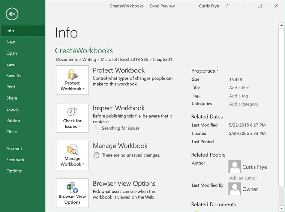
In addition to setting property values on the Info page of the Backstage view, you can display the Properties dialog box to select one of the existing custom categories or create your own. You can also edit your properties or delete any that you no longer want to use.
When you’re finished modifying a workbook, you should save your changes and then close the file.
![]() Tip
Tip
To close a workbook by using a keyboard shortcut, press Ctrl+W.
To create a new workbook
Do any of the following:
If Excel is not running, start Excel. Then, on the Start screen, double-click Blank workbook.
If Excel is already running, click the File tab of the ribbon, click New to display the New page of the Backstage view, and then double-click Blank workbook.
If Excel is already running, press Ctrl+N.
To save a workbook under a new name or in a new location
Click the File tab, and then click Save As.
On the Save As page of the Backstage view, navigate to the folder where you want to save the workbook.
In the Save As dialog box, in the File name box, enter a new name for the workbook.
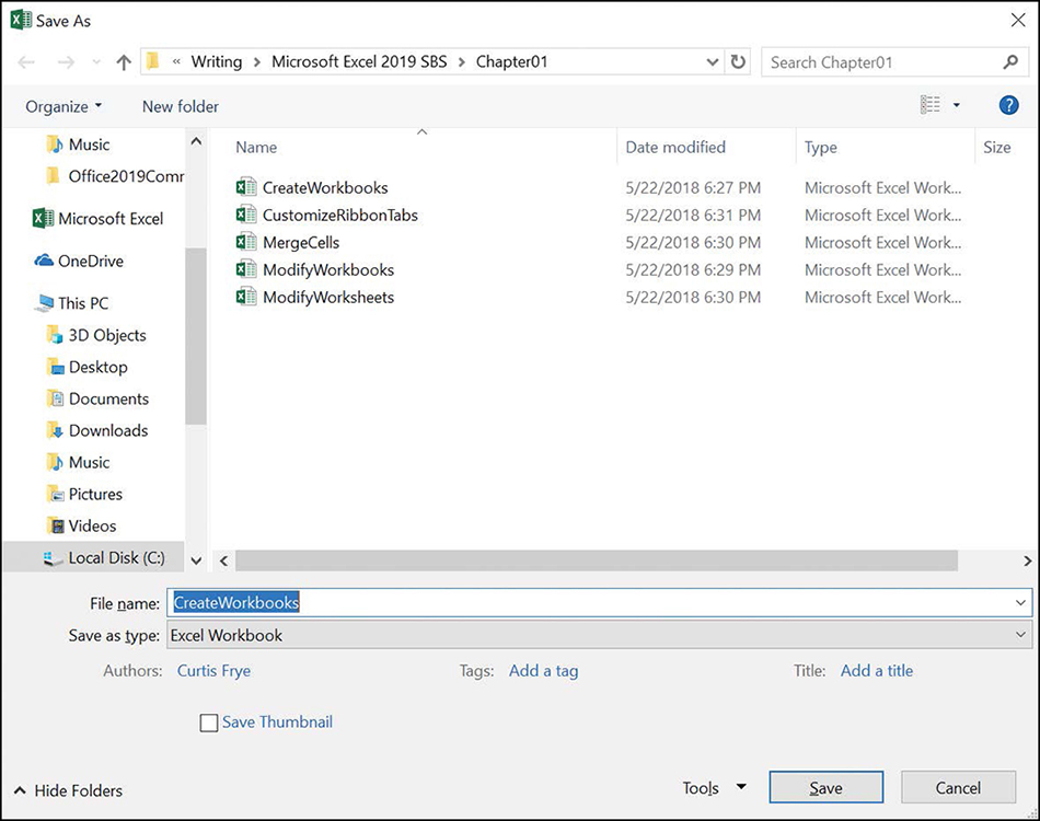
Save a new version of your file using the Save As dialog box. To save the file in a different format, in the Save as type list, click a new file type.
 Tip
TipThe Save as type list contains an extensive list of file formats, including older Excel formats used in Excel 97–2003, macro-enabled workbooks, Comma Separated Value (CSV), and XML Spreadsheet 2003. Not all Excel 2019 features are available in other formats, so be sure your workbook only uses capabilities available in other file formats if you need to use them.
If necessary, use the navigation controls to move to a new folder.
Click Save.
Or
Press F12.
In the Save As dialog box, in the File name box, enter a new name for the workbook.
To save the file in a different format, in the Save as type list, click a new file type.
If necessary, use the navigation controls to move to a new folder.
Click Save.
To open an existing workbook
Click the File tab, and then click Open.
Or
Press Ctrl+O.
On the Open page of the Backstage view, perform any of these actions:
Click a file in the Recent list.
Click another location in the navigation list and select the file.
Click the Browse button, and then use the Open dialog box to find the file you want to open, click the file, and click Open.
To define values for document properties
Click the File tab and, if necessary, click Info.
On the Info page of the Backstage view, in the Properties group, click the Add a property text next to a label.
Enter a value or series of values (separated by commas) for the property.
Click a blank space on the Info page to finish adding properties.
To create a custom property
Click the File tab and then, if necessary, click Info.
In the Properties group, click Properties, and then click Advanced Properties.
In the filename Properties dialog box, click the Custom tab.
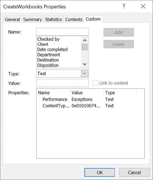
Define custom properties for your workbooks. In the Name list, click an existing property name.
Or
In the Name box, enter a name for the new property.
Click the Type control’s arrow, and then click a data type.
In the Value box, enter a value for the property.
Click Add.
Repeat steps 4–7 to add more properties. When you are finished, click OK.
To close a workbook
Do either of the following:
Display the Backstage view, and then click Close.
Press Ctrl+W.
Modify workbooks
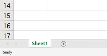
You can use Excel workbooks to record information about specific business activities. Each worksheet within that workbook should represent a subdivision of that activity. To display a particular worksheet, just click the worksheet’s tab (also called a sheet tab) on the tab bar (just below the grid of cells). You can also create new worksheets when you need them.
When you create a worksheet, Excel assigns it a generic name such as Sheet2, Sheet3, or Sheet4. After you decide what type of data you want to store on a worksheet, you should change the worksheet’s name to something more descriptive. You can also move and copy worksheets within and between workbooks. Moving a worksheet within a workbook changes its position, whereas moving a worksheet to another workbook removes it from the original workbook. Copying a worksheet keeps the original in its position and creates a second copy in the new location, whether within the same workbook or in another workbook.
![]() Tip
Tip
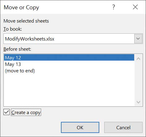
Selecting the Create A Copy check box in the Move or Copy dialog box leaves the copied worksheet in its original workbook, whereas clearing the check box causes Excel to delete the worksheet from its original workbook.
![]() Tip
Tip
You can also copy a worksheet within a workbook by holding down the Ctrl key while dragging the worksheet’s tab to a new position in the workbook.
After the worksheet is in the target workbook, you can change the worksheet’s position within the workbook, hide its tab on the tab bar without deleting the worksheet, unhide its tab, or change the sheet tab’s color.
![]() Tip
Tip
If you copy a worksheet to another workbook and the destination workbook has the same Office theme applied as the active workbook, the worksheet retains its tab color. If the destination workbook has another theme applied, the worksheet’s tab color changes to reflect that theme. For more information about Office themes, see Chapter 4, “Change workbook appearance.”
If you determine that you no longer need a particular worksheet, such as one you created to store some figures temporarily, you can delete the worksheet quickly.
To display a worksheet
On the tab bar in the lower-left corner of the app window, click the tab of the worksheet you want to display.
To create a new worksheet
Next to the tab bar in the lower-left corner of the app window, click the New Sheet button (the plus sign).
To rename a worksheet
Double-click the tab of the worksheet you want to rename.
Enter a new name for the worksheet.
Press Enter.
To move a worksheet within a workbook
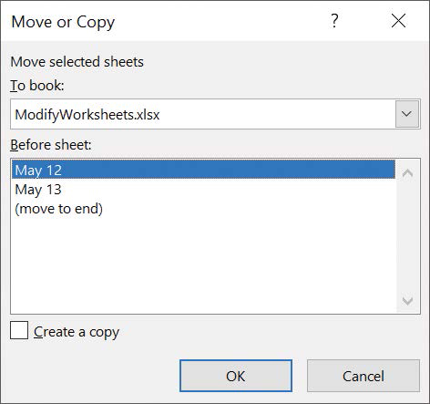
Right-click the sheet tab of the worksheet you want to copy, and then click Move or Copy.
In the Move or Copy dialog box, use the items in the Before sheet area to indicate where you want the new worksheet to appear.
Click OK.
Or
On the tab bar in the lower-left corner of the app window, drag the sheet tab to the new position in the worksheet order.
To move a worksheet to another workbook
Open the workbook to which you want to move a worksheet from another workbook.
In the source workbook, right-click the sheet tab of the worksheet you want to move, and then click Move or Copy.
In the Move or Copy dialog box, click the To book arrow and select the open workbook to which you want to move the worksheet.
In the Before sheet area, indicate where you want the moved worksheet to appear.
Click OK.
To copy a worksheet within a workbook
Right-click the sheet tab of the worksheet you want to copy, and then click Move or Copy.
In the Move or Copy dialog box, select the Create a copy check box.
In the Before sheet area, indicate where you want the new worksheet to appear.
Click OK.
Or
Hold down the Ctrl key and drag the worksheet’s tab to the desired position in the worksheet order.
To copy a worksheet to another workbook
Open the workbook to which you want to add a copy of a worksheet from another workbook.
In the source workbook, right-click the sheet tab of the worksheet you want to copy, and then click Move or Copy.
In the Move or Copy dialog box, select the Create a copy check box.
Copy worksheets to other workbooks without deleting the original sheet. Click the To book arrow and select the open workbook in which you want to create a copy of the worksheet.
In the Before sheet area, indicate where you want the new worksheet to appear.
Click OK.
To hide a worksheet
Right-click the sheet tab of the worksheet you want to hide, and then click Hide.
To unhide a worksheet
Right-click any visible sheet tab, and then click Unhide.
In the Unhide dialog box, click the worksheet you want to redisplay.
Click OK.
To change a sheet tab’s color
Right-click the sheet tab whose color you want to change and point to Tab Color.
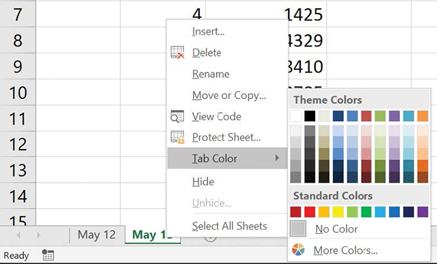
Change a sheet tab’s color to make it stand out. Click a color from the color palette.
Or
Click More Colors, use the tools in the Colors dialog box to pick a color, and then click OK.
To delete a worksheet
Right-click the sheet tab of the worksheet you want to delete, and then click Delete.
If Excel displays a confirmation dialog box, click Delete.
TipExcel displays a confirmation dialog box when you attempt to delete a worksheet that contains data.
Modify worksheets
After you put up the signposts that make your data easy to find, you can take other steps to make the data in your workbooks easier to work with. Excel helps by identifying worksheet rows by number, and columns by one or more letters. Each row has a header at the left edge of the worksheet and each column has a header at the top of the worksheet. You can change the width of a column or the height of a row in a worksheet by dragging the column header’s right edge or the row header’s bottom edge to the position you want. Increasing a column’s width or a row’s height increases the space between cell contents, making your data easier to read and work with.
![]() Tip
Tip
You can apply the same change to more than one row or column by selecting the rows or columns you want to change and then dragging the border of one of the selected rows or columns to the location you want. When you release the mouse button, all the selected rows or columns change to the new height or width.
Modifying column width and row height can make a workbook’s contents easier to work with, but you can also insert a row or column between cells that contain data to make your data easier to read. Adding space between the edge of a worksheet and cells that contain data, or perhaps between a label and the data to which it refers, makes the workbook’s contents less crowded.
![]() Tip
Tip
Inserting a column adds a column to the left of the selected column or columns. Inserting a row adds a row above the selected row or rows.
When you insert a row, column, or cell in a worksheet that has had formatting applied, the Insert Options button appears. Clicking this button displays a list of choices you can make about how the inserted row or column should be formatted. The following table summarizes these options.
Chapter |
Chapter |
|---|---|
Format Same As Above |
Applies the formatting of the row above the inserted row to the new row |
Format Same As Below |
Applies the formatting of the row below the inserted row to the new row |
Format Same As Left |
Applies the formatting of the column to the left of the inserted column to the new column |
Format Same As Right |
Applies the formatting of the column to the right of the inserted column to the new column |
Clear Formatting |
Applies the default format to the new row or column |
You can also delete, hide, and unhide columns and rows. Deleting a column or row removes it and its contents from the worksheet entirely, whereas hiding a column or row removes it from the display without deleting its contents.
![]() Important
Important
If you hide the first row or column in a worksheet and then want to unhide it, you must click the Select All button in the upper-left corner of the worksheet (above the first row header and to the left of the first column header) or press Ctrl+A to select the entire worksheet. Then, on the Home tab, in the Cells group, click Format, point to Hide & Unhide, and click either Unhide Rows or Unhide Columns to make the hidden data visible again.
Just as you can insert rows or columns, you can insert individual cells into a worksheet. After you insert cells, you can use the Insert dialog box to choose whether to shift the cells surrounding the inserted cell down (if your data is arranged as a column) or to the right (if your data is arranged as a row).
![]() Tip
Tip
The Insert dialog box also includes options to insert a new row or column; the Delete dialog box has similar options for deleting an entire row or column.
If you want to move the data in a group of cells to another location in your worksheet, select the cells you want to move and then point to the selection’s border. When the pointer changes to a four-pointed arrow, you can drag the selected cells to the target location on the worksheet. If the destination cells contain data, Excel displays a dialog box asking whether you want to overwrite the destination cells’ contents. You can choose to overwrite the data or cancel the move.
To change row height
Select the row headers for the rows you want to resize.
Point to the bottom border of a selected row header.
When the pointer changes to a double-headed vertical arrow, drag the border until the row is the height you want.
Or
Select the row headers for the rows you want to resize.
Right-click any of the selected row headers, and then click Row Height.
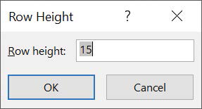
The Row Height dialog box displaying the default row height. In the Row Height dialog box, enter a new height for the selected rows.
TipThe default row height is 15 points.
Click OK.
To change column width
Select the column headers for the columns you want to resize.
Point to the right border of a selected column header.
When the pointer changes to a double-headed horizontal arrow, drag the border until the column is the width you want.
Or
Select the column headers for the columns you want to resize.
Right-click any of the selected column headers, and then click Column Width.
In the Column Width dialog box, enter a new width for the selected columns.
TipThe default column width is 8.09 standard characters.
Click OK.
To insert a column
Right-click a column header, and then click Insert.
To insert multiple columns
Select a number of column headers equal to the number of columns you want to insert.
Right-click any selected column header, and then click Insert.
To insert a row
Right-click a row header, and then click Insert.
To insert multiple rows
Select a number of row headers equal to the number of rows you want to insert.
Right-click any selected row header, and then click Insert.
To delete one or more columns
Select the column headers of the columns you want to delete.
Right-click any selected column header, and then click Delete.
To delete one or more rows
Select the row headers of the rows you want to delete.
Right-click any selected row header, and then click Delete.
To hide one or more columns
Select the column headers of the columns you want to hide.
Right-click any selected column header, and then click Hide.
To hide one or more rows
Select the row headers of the rows you want to hide.
Right-click any selected row header, and then click Hide.
To unhide one or more columns
Select the column headers to the immediate left and right of the column or columns you want to unhide.
Right-click either selected column header, and then click Unhide.
Or
Press Ctrl+A to select the entire worksheet.
Right-click anywhere in the worksheet, and then click Unhide.
To unhide one or more rows
Select the row headers immediately above and below the row or rows you want to unhide.
Right-click any selected column header, and then click Unhide.
Or
Press Ctrl+A to select the entire worksheet.
Right-click anywhere in the worksheet, and then click Unhide.
To insert one or more cells
Select a cell range the same size as the range you want to insert.
On the Home tab of the ribbon, in the Cells group, click Insert.
Or
Right-click a cell in the selected range, and then click Insert.
If necessary, use the controls in the Insert dialog box to tell Excel how to shift the existing cells.
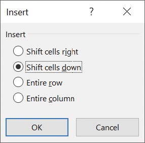
Indicate how Excel should move existing cells when you insert new cells into a worksheet. Click OK.
To move one or more cells within a worksheet
Select the cell range you want to move.
Point to the edge of the selected range.
When the pointer changes to a four-headed arrow, drag the cell range to its new position.
If necessary, click OK to confirm that you want to delete data in the target cells.
Merge and unmerge cells
Most Excel worksheets contain data about a specific subject. One of the best ways to communicate the contents of a worksheet is to use a label.
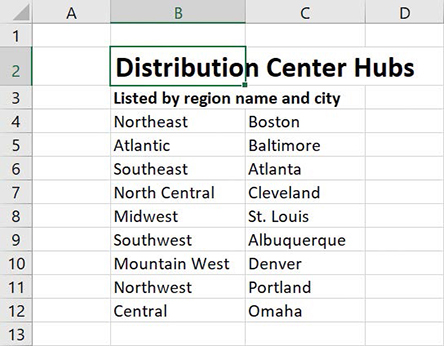
For example, consider a worksheet in which the label text Distribution Center Hubs appears to span three cells, B2:D2, but is in fact contained within cell B2. If you select cell B2, Excel highlights the cell’s border, which obscures the text. You can solve this problem by merging cells B2:D2 into a single cell.
![]() Important
Important
When you merge two or more cells, Excel retains just the text in the range’s upper-left cell. All other text is deleted.
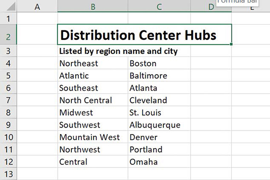
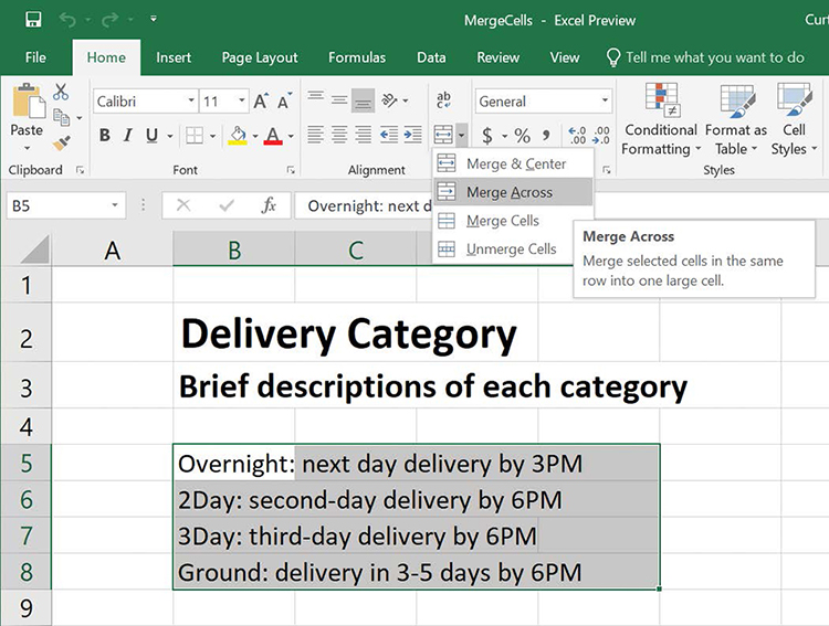
In addition to merging cells, you can click Merge & Center to combine the selected cells into a single cell and center the text within the merged cell. You should consider using the Merge & Center option for label text, such as above a list of data where the title spans more than one column. You can also merge the cells in multiple rows at the same time by using Merge Across.
![]() Important
Important
Selecting the header cells, clicking the Home tab, clicking Merge & Center, and then clicking either Merge & Center or Merge Cells will delete any text that is not in the upper-left cell of the selected range.
If you want to split merged cells into their individual cells, you can always unmerge them.
To merge cells
Select the cells you want to merge.
On the Home tab, in the Alignment group, click the Merge & Center arrow (not the button), and then click Merge Cells.
To merge and center cells
Select the cells you want to merge.
Click the Merge & Center button.
To merge cells in multiple rows by using Merge Across
Select the cells you want to merge.
Click the Merge & Center arrow (not the button), and then click Merge Across.
To split merged cells into individual cells
Select the cells you want to unmerge.
Click the Merge & Center arrow (not the button), and then click Unmerge Cells.
Customize the Excel 2019 app window
How you use Excel 2019 depends on your personal working style and the type of data collections you manage. The Excel product team at Microsoft interviews customers, observes how differing organizations use the app, and sets up the user interface so that many users won’t need to change it to work effectively. If you do want to change the Excel app window, including the user interface, you can. You can zoom in on worksheet data; change how Excel displays your worksheets; add frequently used commands to the Quick Access Toolbar; hide, display, and reorder ribbon tabs; and create custom ribbon tabs to make groups of commands you commonly use readily accessible.
Zoom in on a worksheet
One way to make Excel easier to work with is to change the app’s zoom level. Just as you can zoom in with a camera to increase the size of an object in the camera’s viewer, you can use the zoom setting in Excel 2019 to change the size of objects in the app window. You can change the zoom level from the ribbon or by using the Zoom control in the lower-right corner of the Excel 2019 window. The minimum zoom level in Excel 2019 is 10 percent; the maximum is 400 percent.

To zoom in on a worksheet
Using the Zoom control in the lower-right corner of the app window, click the Zoom In button (the plus sign).
To zoom out on a worksheet
Using the Zoom control in the lower-right corner of the app window, click the Zoom Out button (the minus sign).
To set the zoom level to 100 percent
On the View tab of the ribbon, in the Zoom group, click the 100% button.
To set a specific zoom level
In the Zoom group, click the Zoom button.
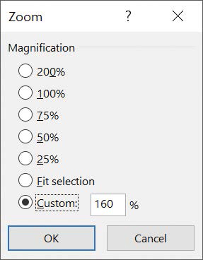
Set a magnification level by using the Zoom dialog box. In the Zoom dialog box, enter a value in the Custom box.
Click OK.
To zoom in on specific worksheet highlights
Select the cells you want to zoom in on.
In the Zoom group, click the Zoom to Selection button.
Arrange multiple workbook windows
As you work with Excel, you might need to have more than one workbook open at a time. For example, you might open a workbook that contains customer contact information and copy it into another workbook to be used as the source data for a mass mailing you create in Word 2019. When you have multiple workbooks open simultaneously, you can switch between them or arrange your workbooks on the desktop so that most of the active workbook is shown prominently but the others are easily accessible.
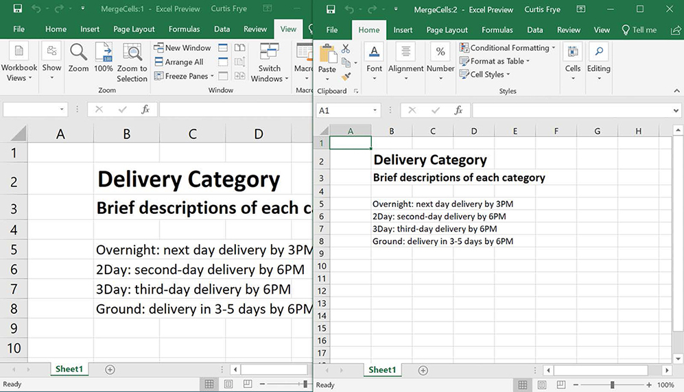
Many Excel 2019 workbooks contain formulas on one worksheet that derive their value from data on another worksheet, which means you need to change between two worksheets every time you want to see how modifying your data changes the formula’s result. To facilitate this, you can display two copies of the same workbook simultaneously, with the worksheet that contains the data in the original window and the worksheet with the formula in a new window. When you change the data in either copy of the workbook, Excel updates the other copy.
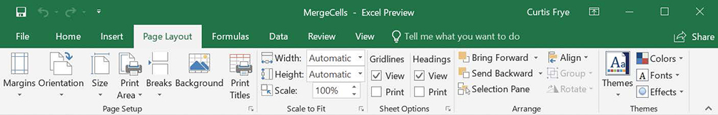
If the original workbook’s name is Merge Cells, Excel 2019 displays the name Merge Cells:1 on the original workbook’s title bar and Merge Cells:2 on the second workbook’s title bar.
To switch to another open workbook
On the View tab, in the Window group, click Switch Windows.
In the Switch Windows list, click the workbook you want to display.
To display two copies of the same workbook
In the Window group, click New Window.
To change how Excel displays multiple open workbooks
In the Window group, click Arrange All.
In the Arrange Windows dialog box, click the windows arrangement you want.
If necessary, select the Windows of active workbook check box.
Click OK.
Add buttons to the Quick Access Toolbar
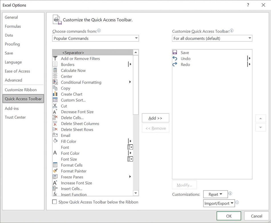
As you continue to work with Excel 2019, you might discover that you use certain commands much more frequently than others. If your workbooks draw data from external sources, for example, you might find yourself using certain ribbon buttons more often than the app’s designers might have expected. You can make any button accessible with one click by adding the button to the Quick Access Toolbar, located just above the ribbon in the upper-left corner of the Excel app window. You’ll find the tools you need to change the buttons on the Quick Access Toolbar in the Excel Options dialog box.
You can add buttons to the Quick Access Toolbar, change their positions, and remove them when you no longer need them. Later, if you want to return the Quick Access Toolbar to its original state, you can reset it.
You can also choose whether your Quick Access Toolbar changes affect all your workbooks or just the active workbook. If you’d like to export your Quick Access Toolbar customizations to a file that can be used to apply those changes to another Excel 2019 installation, you can do so quickly.
To add a button to the Quick Access Toolbar
Display the Backstage view, and then click Options.
In the Excel Options dialog box, click Quick Access Toolbar.
If necessary, click the Customize Quick Access Toolbar arrow and select whether to apply the change to all workbooks or just the current workbook.
If necessary, click the Choose commands from arrow and click the category of commands from which you want to choose.
Click the command you want to add to the Quick Access Toolbar.
Click Add.
Click OK.
To change the order of buttons on the Quick Access Toolbar
Open the Excel Options dialog box, and then click Quick Access Toolbar.
In the right pane, which contains the buttons on the Quick Access Toolbar, click the button you want to move.
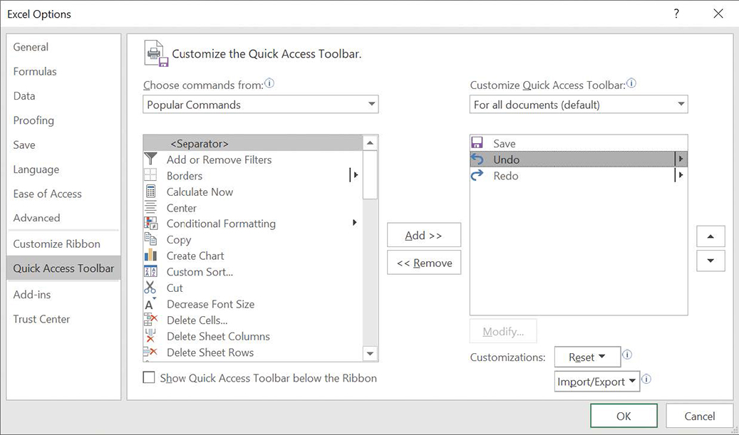
Change the order of buttons on the Quick Access Toolbar. Click the Move Up button (the upward-pointing triangle on the far right) to move the button higher in the list and to the left on the Quick Access Toolbar.
Or
Click the Move Down button (the downward-pointing triangle on the far right) to move the button lower in the list and to the right on the Quick Access Toolbar.
Click OK.
To delete a button from the Quick Access Toolbar
Open the Excel Options dialog box, and then click Quick Access Toolbar.
In the right pane, click the button you want to delete.
Click Remove.
To export your Quick Access Toolbar settings to a file
Display the Quick Access Toolbar page of the Excel Options dialog box.
Click Import/Export, and then click Export all customizations.
In the File Save dialog box, in the File name box, enter a name for the settings file.
Click Save.
To reset the Quick Access Toolbar to its original configuration
Display the Quick Access Toolbar page of the Excel Options dialog box.
Click Reset.
Click Reset only Quick Access Toolbar.
Click OK.
Customize the ribbon
In Excel 2019, you can customize the ribbon user interface. For example, you can hide and display ribbon tabs, reorder tabs displayed on the ribbon, customize existing tabs (including tool tabs, which appear when specific items are selected), and create custom tabs. You’ll find the tools to customize the ribbon in the Excel Options dialog box.
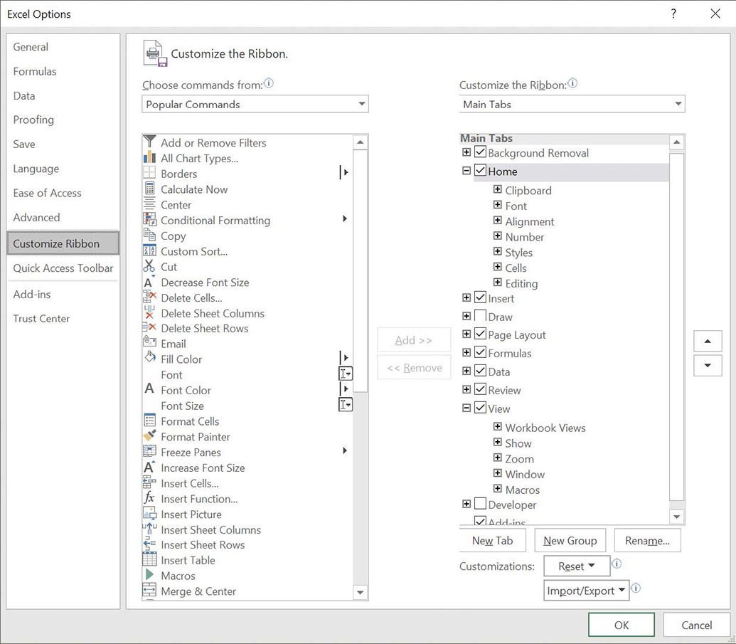
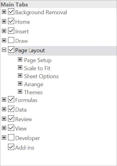
From the Customize Ribbon page of the Excel Options dialog box, you can select which tabs appear on the ribbon and in what order. Each ribbon tab’s name has a check box next to it. If a tab’s check box is selected, that tab appears on the ribbon.
Just as you can change the order of the tabs on the ribbon, with Excel 2019 you can change the order in which groups of commands appear on a tab. For example, the Page Layout tab contains five groups: Themes, Page Setup, Scale to Fit, Sheet Options, and Arrange. If you use the Themes group less frequently than the other groups, you could move the group to the right end of the tab.
You can also remove groups from a ribbon tab. If you remove a group from a built-in tab and later decide you want to restore it, you can put it back.
The built-in ribbon tabs are designed efficiently, so adding new command groups might crowd the other items on the tab and make those controls harder to find. Rather than adding controls to an existing ribbon tab, you can create a custom tab and then add groups and commands to it. The default New Tab (Custom) name doesn’t tell you anything about the commands on your new ribbon tab, so you can rename it to reflect its contents.
You can export your ribbon customizations to a file that can be used to apply those changes to another Excel 2019 installation. When you’re ready to apply saved customizations to Excel, import the file and apply it. And, as with the Quick Access Toolbar, you can always reset the ribbon to its original state.
The ribbon is designed to use space efficiently, but you can hide it and other user interface elements such as the formula bar and row and column headings if you want to increase the amount of space available inside the app window.
![]() Tip
Tip
Press Ctrl+F1 to hide and unhide the ribbon.
To display a ribbon tab
Display the Backstage view, and then click Options.
In the Excel Options dialog box, click Customize Ribbon.
In the tab list on the right side of the dialog box, select the check box next to the name of the tab you want to display.
Select the check box next to the tab you want to appear on the ribbon. Click OK.
To hide a ribbon tab
In the Excel Options dialog box, click Customize Ribbon.
In the tab list on the right side of the dialog box, clear the check box next to the name of the tab you want to hide.
Click OK.
To reorder ribbon elements
In the Excel Options dialog box, click Customize Ribbon.
In the tab list on the right side of the dialog box, click the name of the button or group you want to move.
Click the Move Up button (the upward-pointing triangle on the far right) to move the button or group higher in the list and to the left on the ribbon tab.
Or
Click the Move Down button (the downward-pointing triangle on the far right) to move the button or group lower in the list and to the right on the ribbon tab.
Click OK.
To create a custom ribbon tab
On the Customize Ribbon page of the Excel Options dialog box, click New Tab.
To create a custom group on a ribbon tab
On the Customize Ribbon page of the Excel Options dialog box, click the ribbon tab on which you want to create the custom group.
Click New Group.
To add a button to the ribbon
On the Customize Ribbon page of the Excel Options dialog box, click the ribbon tab or group to which you want to add a button.
If necessary, click the Customize the Ribbon arrow and select Main Tabs or Tool Tabs.
TipTool tabs are contextual tabs that appear when you work with workbook elements such as shapes, images, or PivotTables.
If necessary, click the Choose commands from arrow on the left side of the Customize Ribbon dialog box and click the category of commands from which you want to choose.
Click the command to add to the ribbon.
Click Add.
Click OK.
To rename a ribbon element
On the Customize Ribbon page of the Excel Options dialog box, click the ribbon tab or group you want to rename.
Click Rename.
In the Rename dialog box, enter a new name for the ribbon element.
Click OK.
To remove an element from the ribbon
On the Customize Ribbon page of the Excel Options dialog box, click the ribbon tab or group you want to remove.
Click the Remove button in the middle of the dialog box.
To export your ribbon customizations to a file
On the Customize Ribbon page of the Excel Options dialog box, click Import/Export, and then click Export all customizations.
In the File Save dialog box, in the File name box, enter a name for the settings file.
Click Save.
To import ribbon customizations from a file
On the Customize Ribbon page of the Excel Options dialog box, click Import/Export, and then click Import customization file.
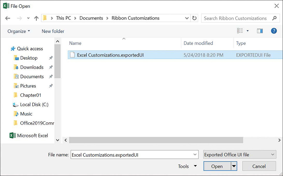
Import ribbon settings saved from another Office installation. In the File Open dialog box, navigate to and select the configuration file.
Click Open.
To reset the ribbon to its original configuration
On the Customize Ribbon page of the Excel Options dialog box, click Reset, and then click Reset all customizations.
In the dialog box that appears, click Yes.
To hide or unhide the ribbon
Press Ctrl+F1.
To hide or unhide the formula bar
On the View tab, in the Show group, select or clear the Formula Bar check box.
To hide or unhide the row and column headings
In the Show group, select or clear the Headings check box.
To hide or unhide gridlines
In the Show group, select or clear the Gridlines check box.
Skills review
In this chapter, you learned how to:
Explore the editions of Excel 2019
Become familiar with new features in Excel 2019
Create workbooks
Modify workbooks
Modify worksheets
Merge and unmerge cells
Customize the Excel 2019 app window
Practice tasks

The practice files for these tasks are located in the Excel2019SBSCh01 folder. You can save the results of the tasks in the same folder.
Create workbooks
Open the CreateWorkbooks workbook in Excel, and then perform the following tasks:
Close the CreateWorkbooks file, and then create a new, blank workbook.
Save the new workbook as Exceptions2018.
Add the following tags to the file’s properties: exceptions, regional, and percentage.
Add a tag to the Category property called performance.
Create a custom property called Performance, leave the value of the Type field as Text, and assign the new property the value Exceptions.
Save your work.
Modify workbooks
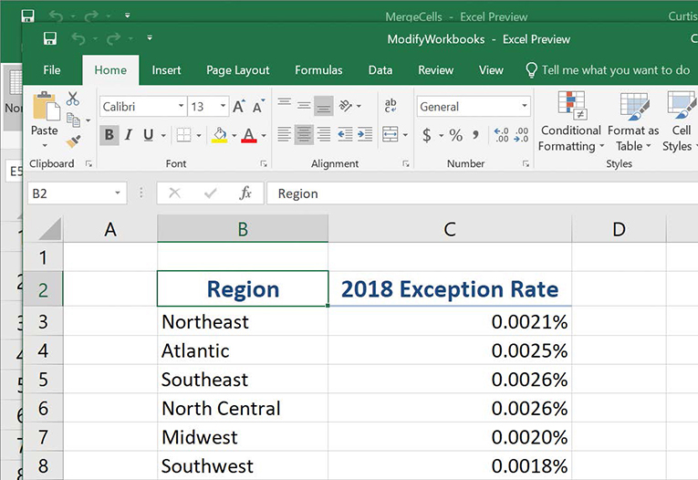
Open the ModifyWorkbooks workbook in Excel, and then perform the following tasks:
Create a new worksheet named 2019.
Rename the Sheet1 worksheet to 2018 and change its tab color to green.
Delete the ScratchPad worksheet.
Copy the 2018 worksheet to a new workbook, and then save the new workbook under the name Archive2018.
In the ModifyWorkbooks workbook, hide the 2018 worksheet.
Modify worksheets
Open the ModifyWorksheets workbook in Excel, and then perform the following tasks:
On the May 12 worksheet, insert a new column A and a new row 1.
After you insert the new row 1, click the Insert Options button, and then click Clear Formatting.
Hide column E.
On the May 13 worksheet, delete cell B6, shifting the remaining cells up.
Click cell C6, and then insert a cell, shifting the other cells down. Enter the value 4499 in the new cell C6.
Select cells E13:F13 and move them to cells B13:C13.
Merge and unmerge cells
Open the MergeCells workbook in Excel, and then perform the following tasks:
Merge cells B2:D2.
Merge and center cells B3:F3.
Merge the cell range B5:E8 by using Merge Across.
Unmerge cell B2.
Customize the Excel 2019 app window
Open the CustomizeRibbonTabs workbook in Excel, and then perform the following tasks:
Add the Spelling button to the Quick Access Toolbar.
Move the Review ribbon tab so it is positioned between the Insert and Page Layout tabs.
Create a new ribbon tab named My Commands.
Rename the New Group (Custom) group to Formatting.
In the list on the left side of the Excel Options dialog box, display the main tabs.
From the buttons on the Home tab, add the Styles group to the My Commands ribbon tab you created earlier.
Again using the buttons available on the Home tab, add the Number group to the Formatting group on your custom ribbon tab.
Save your ribbon changes and click the My Commands tab on the ribbon.