
Embedded systems are usually heterogeneous in that they combine different types of applications. Signal-processing subsystems often have to coexist with control-dominated parts and reactive real-time parts. This means for our discussion that different MoC domains have to be integrated in the system model.
We start this chapter (Section 6.1) with the observation that even two domains, that is, separate process networks, of the same MoC type may have a different time structure. For example, two S-MoC domains that are not connected can have different durations of their evaluation cycles. When connecting them, the relation between their respective time structures has to be defined. This relation can be constant and simple (e.g., 1:1 or 1:3), or it can vary dynamically. The interface processes between the MoC domains define this relation.
Next we define interface processes between different MoC types (Section 6.2). We distinguish between interfaces that add timing information and those that remove timing information. In general, both can be done in many different ways, but we describe only one possible solution.
Based on these interface processes we introduce an integrated MoC (Section 6.3), consisting of different MoC domains and interface processes. Several profound issues emerge when connecting MoC domains, which go beyond the technical insertion and suppression of time information, and we discuss some of them. We propose distinguishing between (1) the time structures of different MoC domains and their relations to each other, (2) the protocol used to model communication between different domains, and (3) the modeling of delays on the channels between different domains (Section 6.4).
After the illumination of some important aspects of interfacing MoC domains, we consider moving functionality between domains (Section 6.5). For the untimed, the synchronous, and the timed MoCs we discuss all possible cases of migrating a process from one domain to another, although some cases are treated only superficially. There are many possible ways to formulate these migrations, and sensible and efficient solutions depend on the application context, which we do not elaborate on further.
Finally (Section 6.6), we take up some possible applications of an integrated MoC. One example is the integration of different front-end languages, such as SDL and Matlab, in a common modeling and design environment. Each front-end language is mapped on a particular MoC, and the integrated MoC is used to define the relation between the different MoCs and thus between the front-end languages.
We have defined three major models of computation and discussed some of their fundamental properties and applications. Since the design of an electronic system usually requires the deployment of different computational models, integration is desirable. The main difficulty obviously is the representation and conversion of timing information. This is an issue even for disconnected process networks of the same MoC. Consider the two process networks in two MoC domains in Figure 6-1. MoC A and MoC B may be the same or different. Only the case where both are the untimed MoC (i.e., MoC A = MoC B = untimed MoC) is unambiguous and unproblematic. Since in both domains there is no timing information present, the two process networks can be directly connected with no need for a special interface. However, if both networks form a perfect synchronous domain (i.e., MoC A = MoC B = synchronous MoC) the elementary timing unit may be different. Since there is no reference to an absolute time in the synchronous MoC, the duration of the basic evaluation cycle may be quite different in MoC A and MoC B. MoC A’s evaluation cycle could have a duration r times that of MoC B’s cycle. r could be a positive integer, but it could also be a rational or real number. In fact, r does not even have to be a constant since the evaluation cycles in a synchronous MoC can vary arbitrarily. This does not become apparent as long as we deal with an isolated domain because there the duration of each evaluation cycle is the same for all processes and it cannot be observed from within the domain whether consecutive cycles vary in length. It can only be observed when compared to another, disconnected domain or some “absolute time reference.” Thus, in the general case, interfaces I1 and I2 in Figure 6-1 could be completely asynchronous even if both domains are perfectly synchronous MoC domains.
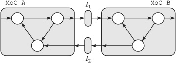
Figure 6-1. The interfaces I1 and I2 define the relation between different MoC domains. All interfaces between two domains must be consistent with each other.
A practically useful case, however, is when r is a constant positive integer, r ∊ N. The following interface constructors can be used to interface synchronous domains in this case:
with

with
length(f(ā)) = 1
ā ∊ ![]() ,r ∊ N
,r ∊ N
intSup emits r events for each input event, and function f defines the values of the emitted events. intSdown emits one event for r input events. Hence, assuming MoC A operates at a rate two times the rate of the MoC B domain in Figure 6-1, we could define the interface processes as follows:
I1 = | with f1(〈 ē1, ē2 〉) = ē1 |
I2 = | with f2(ē) = 〈ē,⊔〉 |
It is obviously crucial that all interfaces between two domains are consistent, which for the special case of constant integer factors r is straightforward to check. Figure 6-2 shows an example of three MoC domains. Their relative cycle period ratio, r1, r2, r3, annotates the connecting arcs. Obviously different arcs connecting two domains must express the same ratio. Hence, the two arcs connecting MoC A and MoC C have the same ratio r3, with one being based on intSup and the other on intSdown. It is interesting to note that the MoC domain graph can be viewed as a synchronous dataflow graph (Section 3.15), and SDF techniques can be used to check consistency in the graph and to determine buffer requirements on domain boundaries.

The situation for connecting two separate clocked synchronous MoC domains or two timed MoC domains is exactly the same as for the perfectly synchronous case. Even though the time granularity or assumptions about computation delays are different, the main issue again is to relate the relative time base in different domains to each other. Thus we can define
Without going into more details, it is obvious that this is closely related to the problem of designing a hardware circuit with multiple clock domains.
If MoC A and MoC B in Figure 6-1 are different MoCs, the interfaces have to bridge domains with different information content concerning time. Consequently interfaces have to filter out or insert timing information. This can be done in many different ways depending on the modeling objectives. Unfortunately we cannot give a systematic presentation of the choices, but we present only selected, simple solutions.
Interface processes that connect processes with different timing regimes either remove or add timing information. Interface constructors that add timing information are labeled with the prefix insert; those that remove timing information have the prefix strip. Table 6-1 lists the names of process constructors that instantiate interface processes. We define them in the following sections.
Table 6-1. Interface processes between timing regimes.
From/to | Timed | Synchronous | Untimed |
|---|---|---|---|
Timed | — |
|
|
Synchronous |
| — |
|
Untimed |
|
| — |
The strip-based processes remove the timing information that they receive on their input signals. This is straightforward when the output signal is an untimed signal because then only the ⊔ symbols have to be removed and other events are passed to the output in the same order they appear at the input.
Example 6.1.
stripT2U is a process constructor that instantiates a process p: Ŝ → ![]() , which is defined as follows:
, which is defined as follows:
stripT2U() = p
where

Example 6.2.
stripS2U is a process constructor that instantiates a process p: Ŝ → ![]() , which is defined as
, which is defined as
stripS2U = stripT2U
However, stripT2S-based processes need additional information to determine the time relation between timed and synchronous events. We use a parameter λ ∊ N that defines the number of events in the timed input signal for each synchronous output event.

This is not the only way to define interface processes between the timed and the synchronous domains. It is easy to imagine the usefulness of processes with a control input that determines the time relation between input and output signals.
For insert-based processes we have to decide on the ratio of input events to output events. This ratio may vary and may be context dependent. However, here we adopt the simple solution with a constant ratio λ.
Example 6.4.
insertU2S is a process constructor that, given a natural number λ, instantiates a process p: ![]() →
→ ![]() , defined as follows:
, defined as follows:
insertU2S(λ) = p
where
p( | = |
π(ν, | =〈ėi〉, ν(i) = 1 |
π(ν′, | =〈āi〉, ν′(i) = λ |
āi | = 〈ėi〉 ⊕ 〈⊔〉λ−1 |
for λ ∊ N, | |
We now have the means to reason about all three computational models in a unifying framework. Before we formulate an MoC that contains several MoC domains, we generalize the MoC concept.
Example 6.7.
A hierarchical model of computation (HMoC) is a 3-tuple HMoC = (M, C, O), where
M is a set of HMoCs, each capable of instantiating processes;
C is a set of process constructors, each of which, when given constructor-specific parameters, instantiates a process;
O is a set of process composition operators, each of which, when given processes as arguments, instantiates a new process.
By “process” we mean either an elementary process or a process network.
This allows us to formulate hierarchical MoCs with specialized MoC domains in a structured way.
Example 6.8.
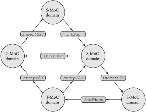
The integrated model of computation (integrated MoC) is defined as integrated HMoC = (M, C, O), where
M = {U-MoC, S-MoC, T-MoC}
C = {intSup, intSdown, intTup, intTdown, stripT2S, stripT2U, stripS2U, insertS2T, insertU2T, insertU2S}
O = {||, o, FBP}
In other words, a process or a process network belongs to the integrated MoC domain iff all its processes and process compositions are constructed either by one of the named MoCs, one of the process constructors, or by one of the composition operators. We call such processes I-MoC processes.
We use the feedback operator FBp, which is based on the prefix order of signals, to define the semantics of feedback loops. In the synchronous MoC we have used the FBS operator based on the Scott order of values. As a result we have different semantics in the different subdomains. This is not a problem, however, because the process network in a subdomain is viewed from the outside as just another process. The interior of this process is of no concern to the outside as long as it complies at the interfaces with the expectations of the surrounding processes. Although it is not formally required in Definition 6.8, we have to constrain models such that proper interfaces are always used for connecting subdomains, as is the case in Figure 6-3. Thus, if a S-MoC domain is surrounded by proper interface processes, its internal semantics does not cause inconsistencies with other subdomains.
Example 6.1.
As an example with two MoC domains, we consider a digital equalizer system (Bjuréus and Jantsch 2000), illustrated in Figure 6-4. We only discuss the highest hierarchical level, consisting of four processes. The Filter process reads the primary input, an audio signal, in chunks of 4096 data points. The Filter contains high-pass, band-pass, and low-pass filters and amplifiers. The amplifiers are controlled by the Button control process. Button control receives control inputs from a user interface, which sets the amplification for volume, bass, and treble of the output audio signal. The output of Filter is analyzed by the Analyzer process with the goal of detecting harmful output signals to avoid damaging the loud speakers. The Distortion control process uses the result of the Analyzer and provides input to the Button control, which in turn sets the parameters for the Filter.
Figure 6-4 shows the process graph. The inputs and outputs of each process are annotated by the number of events consumed and emitted in each evaluation cycle. The interfaces between the two domains are simple. They establish a one-to-one correspondence between the untimed and the synchronous events on their inputs and outputs. The interface from S-MoC to the U-MoC domain uses a process I in addition to stripS2U, defined as follows:
I = mapS(f)
with

I replaces absent events with 0, meaning that the control values in the Filter should not change.
This digital equalizer is quite typical: it has a datapath with a regular dataflow and a control part with relatively few control events occurring at irregular points in time. Input to the Distortion control arrives periodically triggered by the activity in the datapath. But its output and the inputs and the output of the Button control process will occur very rarely and irregularly depending on user inputs and on the need to change Filter parameters.

Figure 6-4. The digital equalizer system consists of a control part, modeled in S-MoC, and a dataflow part, modeled in U-MoC.
As this is a very typical situation, it is worth while to carefully examine the choices we have to link the two domains. First, we observe that, by connecting the two domains, the untimed processes take on a notion of time. Suddenly, the activities of the untimed processes can be related to the time of the synchronous domain. But could the interfaces, which are very simple in our example, be designed differently to avoid this coupling? The answer is no for the modeling devices we have introduced so far. Since the overall equalizer system is deterministic, we have to decide and describe precisely how the output of the Analyzer is merged into the time fabric of the synchronous domain. Similarly, the activity of the Filter process is pressed into the time fabric originating from the Button control process. This effect propagates to all untimed processes, even those not directly connected to the S-MoC domain.
Is this coupling effect the result of all the untimed processes imposing constant partitionings on their input and output signals? Consider the case where the Analyzer emits data only when the current analysis result is different from the previous one (Figure 6-5). The consequence would be that the entire time structure of the S-MoC domain would be aligned with the output of the Analyzer. This would be an unpleasant situation because it would make the operation of the Button control and of the Filter processes dependent on Analyzer output. Recall that the timing structure in the S-MoC is determined by the primary inputs. Consequently, all the inputs to a synchronous domain must have a consistent timing structure, which is not the case if the timing structure on one input is completely dependent on the datapath activity, and the other input, coming from a user interface, is rooted in the time structure of the real world.

Hence, when untimed processes have a variable and dynamic partitioning of their signals, the timing structure can radically change, but the coupling effect to the synchronous domain is not decreased. The conclusion is that we must interpret the activities of the untimed processes with respect to a time structure if we want to connect them to a synchronous or timed MoC domain.
This consequence may contradict the ambition of keeping considerations of time out of the untimed domain and restricting time effects to the synchronous or timed domain. Perhaps at this point you are thinking that an asynchronous interface, which reads data from the untimed domain whenever it arrives, is called for. However, an asynchronous interface can only connect two domains that both have a time structure, albeit two different and uncorrelated time structures. If one domain has no time structure whatsoever, an asynchronous interface does not help. Its introduction would only link the two domains and establish correlated, but not necessarily synchronized, time structures in both domains.
We can make the coupling more flexible by adding nondeterminism into the interface. Figure 6-6 indicates this possibility.[1] Process R inserts a nondeterministic number of absent events between every two events from the Analyzer. Similarly, we can add a nondeterministic element to I, the other domain interface process in Figure 6-4. I could emit a nondeterministic number of zeroes for each consumed absent event. Doing so would nondeterministically vary the delay between the control part and the datapath. It would not avoid, however, imposing a timing structure on the untimed domain.

Figure 6-6. The interface process R inserts a random number of absent events between two events from the Analyzer.
Assume R adds 100 absent events between two particular data events, e1 and e2, from the Analyzer. The effect of e2 would appear at the input of the Filter 100 S-MoC evaluation cycles after the effect of e1. However, in the meantime Filter would have received 100 zero-events, one for each absent event, from the controller. It would have continued its operation, that is, evaluating 100 chunks of the input signal. Thus, the obvious interpretation is that there is a clear and unambiguous time relation between the untimed and the synchronous domains. By adding delays in the interfaces nondeter-ministically, we can model nondeterministic delay, but we would still import a timing structure from the synchronous into the untimed domain.
In summary, we can conclude that by connecting two MoC domains, we relate their time structure to each other. Untimed MoC domains import a time structure from synchronous or timed domains. It is crucial that the correlation between the involved time structures, which is determined by the interfaces, is in fact the one desired by the designer. Moreover, it is imperative that all the interfaces are consistent with each other. We do not yet have a systematic method to support the designer in achieving all this. But techniques and tools exist that address specific instances of this general problem. For example, Jantsch and Bjuréus (2000) have developed a modeling environment and a methodology to integrate the timed MoC defined by SDL (Olsen et al. 1995) with the untimed model of the Matlab (Hanselman and Littkefield, 1998) language.
As elaborated above, when two MoC domains are connected, their time structures are set in a particular relationship to each other. How shall we model the situation where we do not make assumptions about this relationship, but we still want to design a reliable communication? We propose the following three-step procedure:
Add a time interface: To connect two MoC domains, whether of the same or of different types, we have to use an interface that defines the relationship of the time structure. Examples are the interface constructors
intSup,stripT2U,insertU2S, and so on, introduced earlier. They usually establish a constant and fixed relationship. This is not a necessity, however. Consider the following interface constructor:intSups(r, s, f′, f″) =mealyU(1, f, g,0)with

intSupsis just likeintSupexcept that every s cycles it emits r + 1 events rather than r. For these two different situations, the two functions f′ and f″ are used. This can capture the case where the frequencies in the two MoC domains are not a simple multiple of each other. s could even be modeled as a stochastic variable to account for fluctuations in the relationship of the two time structures. Hence, there is considerable flexibility in defining the time relationship between the two domains, but nevertheless it should be defined precisely.Refine the protocol: Model the asynchronous protocol that will provide the reliable communication between the two MoC domains.
Model the channel delay: If the channel is subject to delay variations, use a stochastic process to model the channel delay. Stochastic processes will be introduced in Chapter 8.
Example 6.2.
To illustrate this procedure, consider the communication between processes P and Q in two different timed MoC domains, MoC A and MoC B, respectively (Figure 6-7). Both P and Q are simple identity processes, passing their inputs unchanged to their outputs. The time structure relationship, as defined by the interface I1, is such that two evaluation cycles in MoC A correspond to three cycles in MoC B. f1 and f2 are defined as
f1(ê) | = 〈ê, ⊔, ⊔〉 |
f2(〈⊔, ⊔〉) | = ⊔ |
f2(〈⊔, ê〉) | = ê |
f2(〈ê, ⊔〉) = ê
f2(〈ê1, ê2〉) = ê1
In the second step of the procedure we model a protocol that is robust to changes in the time structure relationship. Figure 6-8 shows how P is refined into two processes, P1 and P2, and Q is refined into Q1 and Q2. We can reuse the interface I1 for the communication from MoC A to MoC B. For the opposite direction we have to design a corresponding interface process I2:
I2 = intTdown(3, f4) o intTup(2, f3)
with
f3(ê) = 〈ê, ⊔〉
f4(⊔, ⊔, ⊔) = ⊔
f4(〈ê,_,_〉) = ê
f4(〈⊔, ê,_〉) = ê
f4(〈⊔, ⊔, ê〉) = ê
The “_” symbol indicates a wild card matching any value or event including the absent event.
I2 implements a time structure relationship consistent with I1, but care has to be taken because events may get lost in I2, while events can never be lost in I1.
Process P and Q are refined into processes P1, P2, Q1, and Q2 as defined in Figures 6-8 and 6-9. The main idea is as follows:P1 packs the primary input data and a control signal from Q1 into an event that is then processed by P2. The only possible value of the control event from Q1 is an acknowledgment ack. After P2 has sent a valid data to Q2, it awaits an ack event before sending new data. P2 does not buffer any data. Thus, if new data arrives while P2 is waiting for an acknowledgment, it is silently dropped. A buffer of any size could, of course, be added to avoid loss of data, but we have suppressed it to keep the model simple. When P2 sends valid data, it also sends a control event, valid.
Q1 is a simple unzip process separating the primary data output signal from the acknowledgment signal for the handshake procedure. Q2 is a stateless process that emits an acknowledgment event for every valid data event it receives.
The handshake protocol, as simple as it may be, illustrates step 2, the refinement of an abstract channel into a concrete protocol implementation.
Step 3 introduces a delay model of the channel between the two domains. In Figure 6-10 two processes, labeled D[2,5], are inserted into the interface between the two MoC domains. They are stochastic processes and delay events by two to five cycles. Since we will introduce stochastic processes only in Chapter 8, we will not provide further details here. A deterministic delay could be easily modeled with initT-based processes.
If you have been observant, you will have certainly noted that the handshake protocol does not work correctly because the interface I2 drops some events since it receives more events than it emits. See Exercise 6.1 to rectify this error.

Figure 6-7. Processes P and Q in two different timed domains are connected via the interface I1 = intTdown(2,f2) o intTup(3,f1).

Table 6-9. P1 simply zips the data input and the control signal from Q1 together. P2 waits for an acknowledgment before sending new data to Q2.
P1 = zipUs(1,1)                                 Q1 = unzipT()
P2 = mealyT(1,f,g,idle)                         Q2 = mapT(1,f)
   with      f(idle,(ê, _)) = (ê, valid)          with         f(⊔) = ⊔
            f(idle(⊔, _))  = ⊔                         f((_, ⊔)) = ⊔
        f(waiting, (ê, ⊔)) = ⊔                       f((ê, valid)) = (ê, ack)
      f(waiting, (⊔, ack)) = ⊔
       f(waiting, (ê, ack)) = (ê, valid)
            g(idle, (ê, _)) = waiting
           g(idle, (⊔, _)) = idle
        g(waiting, (ê, ⊔)) = waiting
      g(waiting, (⊔, ack)) = idle
g(waiting, (ê, ack)) = waiting |

In summary, we advocate separating channel delay modeling, or delay modeling in general, from the relationship of time structures. Whenever separate MoC domains are connected, their time structure is related. It is worth while defining this relationship explicitly and carefully. Doing this, however, should not be confused with defining and modeling the delays between the MoC domains.
One of our objectives is to capture the different computational models in a uniform way, such that the characteristics in each domain are preserved but both optimizations and verification can be done across domain boundaries. A necessary requirement for this, in addition to well-defined interface processes, is that processes can be moved from one domain into another.
Figure 6-11 shows one example of a process moving from the untimed domain into the synchronous domain. Apparently, the process must change in order to preserve the overall system behavior.
Based on the three computational models and the interface processes we have defined, we briefly discuss all the possible migrations for processes with one input and one output signal. All these cases are listed in Table 6-2.
Table 6-2. Migration of processes between timing regimes.
1a. | P | ⇒ | PS o P |
b. | PS o P | ⇒ | P |
2a. | P | ⇒ | PT o P |
b. | PT o P | ⇒ | P |
3a. | P | ⇒ | PT o P |
b. | PT o P | ⇒ | P |
4a. | P | ⇒ | PS o P |
b. | PT o P | ⇒ | P |
5a. | P | ⇒ | PU o P |
b. | PU o P | ⇒ | P |
6a. | P | ⇒ | PU o P |
b. | PU o P | ⇒ | P |
Before we discuss the individual cases, however, we need some supporting processes to describe the migrations concisely.
The process par_c is a synchronous process that takes c consecutive events and packs them into one event as a record or sequence:
par_c = mealyS(f, g, 〈〉)
where

For par_c the number of events to be packed into a record is constant. But for par it is variable and given by a second input. Whenever the first event of a new record arrives at the first input signal, it is expected that the other input signal provides the number that defines the size of this record. par consists of two processes: the first zips the two inputs together, and the second performs the packing.
par = p1 o p2
p1 = zipS()
p1 = mealyS(f, g, (〈〉, 0))
where

The ser process is the inverse operation. It serializes sequences that come in a single event. Recall that tail returns all elements of a sequence except the first one and head returns only the first element of a sequence.
ser = mooreS(f, g, 〈〉)
where

In the following, we discuss 12 cases that should be considered as examples rather than a systematic methodology. As will be seen, the best solution on how to transform the migrated processes and the interfaces depends on the details of the processes and the concrete context. Therefore, a designer would like to have a rather large library of migration patterns available from which specific solutions can be selected and parameterized.
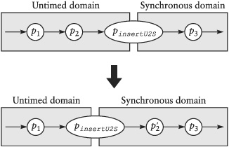
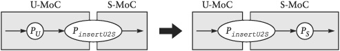
Case 1a: (PinsertU2S o PU ⇒ PS o PinsertU2S)
Consider two processes connected together: pI o p (Figure 6-12). First, we discuss the migration of a stateless process. Let p be a mapU -based untimed process and pI be an interface process from the untimed to the synchronous domain.
p = mapU(c, f1)
pI = insertU2S(1)
Then the two processes can be transformed into pI o q, with q being defined as follows:

Because the original process p takes c events during each execution cycle, but a synchronous process can only take one, we have to pack c event values into one record event (by q1) before we can apply the original function f1 on these records (done by q2 and f2). Similarly, because the untimed process p can generate any number of output events, we have to serialize the resulting value records into individual synchronous events, which is done by q3.
If p is a process with state, the migration is more involved. Let p = mealyU (γ, f, g, w0). Process p and pI are, as above, connected together, pI o p.
p = mealyU(γ, f, g, w0)
pI = insertU2S(1)
Then, they can be transformed into processes q o pI, where q is a process consisting of five subprocesses as depicted in Figure 6-13.

Figure 6-13. The process resulting from the migration of a Mealy-based process from the untimed into the synchronous domain.
Process q1 parallelizes the incoming events. q2 represents the scan part of the process p; thus it contains the internal state and updates it. q3 is the output encoder.
Next-state processing and output encoding had to be separated because we need the information concerning how many events should be assembled into the next record by q1. To infer this we need access to the internal state, which is now visible at signal s3. Process q5 infers this information and provides q1 with the record sizes. Finally, q4 serializes the packed events.
More formally, the process q is defined as follows:
q(s1) = s5
where
s5 = q4(s4)
s4 = q3(s3, s2)
s3 = q2(s2)
s2 = q1(s1, s6)
s6 = q5(s3)
q1 = par
q2 = scanS(f2, w0)
where

where

Case 1b: (PS o PinsertU2S ⇒ PinsertU2S o PU)
In general it is difficult to fully emulate a synchronous process in the untimed domain because its behavior may depend on timing information that is not available for untimed processes. It is much simpler to move a process the opposite way from the synchronous into the untimed domain. As elaborated below for case 2b, we have two options to deal with this problem. However, for the special case λ = 1, the following transformation fully preserves the behavior.
Consider two processes connected together:
p o pI
with
pI = insertU2S(1)
p = mealyS(f, g, w0)
We can easily transform them into
pI o q
with
q = mealyU(1, f, g, w0)
Case 2a: (PinsertU2T o PU ⇒ PT o PinsertU2T)
Migrating a process from the untimed into the timed domain is easier than moving it into the synchronous domain because both the timed and untimed processes can consume an arbitrary number of events in each firing cycle. Again we only consider the special case where the interface process provides a time ratio of λ = 1.
Two processes, p = mealyU (γ, g, f, w0) and pI = insertU2T(1), which are connected together (pI o p), can be transformed into two other processes q o pI if q is defined as q = mealyT(γ, g, f, w0). If λ is not 1, we could still have the new interface process with λ = 1 and process q generate absent events in the same way as the interface process does. This exactly preserves the behavior and the timing. In many practical cases the preservation of the timing may not be required, allowing transformations that result in simpler processes.
Case 2b: (PT o PinsertU2T ⇒ PinsertU2T o PU)
In contrast to case 2a this transformation is a difficult issue. The reason is that we simply cannot emulate the full behavior of a timed process by an untimed process. The timed process’s behavior may depend on the timing of the input events, and the timing of the output events may be an essential part of the behavior. There are two approaches to address this situation. First, we could encode and preserve the timing information in the untimed domain, for example, by representing absent events with a special data value that is not used otherwise or by annotating each event with a time tag. This would allow us to fully emulate the timed process’s behavior in the untimed domain at the expense of increased complexity of the untimed process. Second, we could ignore the timing information and only emulate the timed process’s behavior as far as it depends on the values and sequence of events but not on their timing. This will only be possible if these two aspects are already separated to some degree in the timed domain.
However, we will abstain from developing these ideas and leave as future work the development of a set of practically useful transformations that allow designers to choose the most appropriate approach for a given problem.
Case 3a: (PinsertS2T o PS ⇒ PT o PinsertS2T)
Two processes, p = mealyS(g, f, w0) and pI = insertS2T(λ), which are connected together (pI o p), can be transformed into two other processes q o p′I if q and p′I are defined as follows:
p′I = insertS2T(1)
q = mealyT(1, g, f′, w0)
where
f′ (w, ê) = f (w, ê) ⊕〈⊔〉λ−1
We have simply integrated both p and the pI into the new process q while simplifying the new interface process.
Case 3b: (PT o PinsertS2T ⇒ PinsertS2T o PS)
Similarly to case 1a, we have to deal with the situation where the timed process can consume and produce any number of events, while the constructed synchronous process can consume and produce only one event at a time. Hence, we must parallelize events before the synchronous process and serialize them after the synchronous process. Again, we consider only the special case with a time ratio λ = 1.
Let p = mealyT(γ, f, g, w0) and pI = insertS2T(1) be connected together, p? pI. They can be transformed into processes pI o q, where q is a process consisting of five subprocesses as depicted in Figure 6-13 and derived in exactly the same way as in case 1a.
Case 4a: (PstripT2S o PT ⇒ PS o PstripT2S)
We again have a similar situation as in cases 1a and 3b where we had to parallelize the input in the synchronous domain to emulate the behavior of the timed and untimed processes. The same scheme as we employed in the earlier cases can be used here for the situation of a time ratio of λ = 1.
Case 4b: (PS o PstripT2S ⇒ PstripT2S o PT)
The stripT2S process filters out all events except the last in a clock cycle as determined by λ. When we move a synchronous process upwards against the data stream across a stripT2S process and transform it into a timed process, the new process will potentially see many more events. However, since the interface process filters events based only on their timing, we can make the data processing also in the timed domain provided that the timed process does not rely on detailed timing information. Hence, this transformation is fairly simple but may lead to the unnecessary processing of many events in the timed domain.
Given are two processes, p = mealyS(g, f, w0) and pI = stripT2S(λ), which are connected together, p o pI. These two processes can be transformed into two other processes p′I o q, defined as follows:
q = mealyT(λ, g′, f′, w0)
where
g′ (w, â) = g (w, lastt(â))
f′ (w, â) = f (w, lastt(â))
p′I = stripT2S(1)
Case 5a: (PstripT2U o PT ⇒ PU o PstripT2U)
Again, as in case 1b and 2b, this transformation is in general not possible because the necessary information (i.e., the time information) is not available to the untimed process.
Case 5b: (PU o PstripT2U o PstripT2U o PT)
Since the untimed process operates only on the nonabsent events, we can emulate its behavior in the timed domain by ignoring all absent events. Conveniently, we filter absent events in a separate process that resembles the interface process.
Let p = mealyU (γ, g, f, w0) and pI = stripT2U () be connected together, p o pI. They can be transformed into processes pI o q with
q = q1 o q2
q2 = mapT(1, f)
where

Case 6a: (PstripS2U o PS ⇒ PU o PstripS2U)
As in cases 1b, 2b, and 5b, the full behavior of a synchronous process is difficult to emulate in the untimed domain due to a lack of timing information.
Case 6b: (PU o PstripS2U ⇒ PstripS2U o PS)
We can completely emulate the behavior of the untimed process in the synchronous domain, but as in case 1a we have to properly parallelize the incoming events first and serialize them after processing. We can use the same scheme as in case 1a, but in addition we have to filter out all absent events before the parallelization.
The process migration techniques described here are merely examples and are not developed in a systematic way for two reasons. First, the details of such a transformation often depend on the application and on the context. To make a process migration useful and feasible, context- and application-specific information has to be used, which may not always be explicit in the model at all. Second, we just do not have the understanding and practical experience with inter-domain process migration. The systematic development of a set of techniques and tools to support process migration and cross-domain formal verification of functionality and performance figures is still an area open for research.
Traditionally, the term “model of computation” has been used to intuitively describe different concepts of communication and synchronization between concurrent processes. Occasionally, interfaces between different models of computation have been defined to allow the joint simulation of processes in different MoC domains. Ptolemy is the most prominent example of a framework that integrates a number of different models of computation for the purpose of simulation and modeling.
Our formal framework attempts to study the integration of different MoCs on a more fundamental level—to go beyond simulation and eventually address integrated synthesis, optimization, and verification across various MoCs. Since this is a long-term research program, we only want to sketch some possible concrete applications.
First, the framework is a means to study the relationships between different MoCs. Technically we have introduced the framework as a dataflow process network without timing information. Other MoCs have been embedded in this framework by introducing a particular data type, the absent event, which is interpreted by processes as timing information. Hence, all MoCs are formulated in the same semantic framework and can therefore be easily studied together. For instance, we have formulated the dataflow process network with firing rules (Lee 1997) in our framework. It can then be shown that the U-MoC contains a strictly larger set of processes because the partitioning function for the input signal need not be bounded in the number of events consumed in an evaluation cycle while the firing rules require bounded input partitionings.
The composite signal flow model (Jantsch and Bjuréus 2000) is another example of the integration of MoCs. It allows us to model both untimed and timed processes and their interaction with the same formalism. It has been successfully applied to integrating the design languages Matlab and SDL into a common modeling environment (Bjuréus and Jantsch 2001). The same can be achieved in our framework since both formalisms are very similar. Again, the composite signal flow can be formulated in our framework as a particular MoC, and its expressive power can be compared with the timed MoC. The composite signal flow is also a good example of how a formal foundation for a computational model can be used to facilitate the practical task of integration of different design tasks and languages that have no formal relationship to each other per se. As illustrated in Figure 6-14, each of the design languages has to be mapped onto a particular MoC. Then interface processes between the resulting MoCs have to be designed, and the communication between the design languages has to be implemented in compliance to the semantics of the interface processes. The implementation of the communication is typically glue code using the foreign language interfaces of the involved simulators. In the SDL-Matlab case, both the Matlab execution environment and the SDL simulator allow the inclusion of arbitrary C code, which is used to establish a connection between the two environments and implement the communication.

The mapping of a design language onto an MoC may not be complete either because some language features are not relevant for the task at hand or because the language contains features that cannot easily be expressed in an MoC framework. This may lead to a modeling technique restricting the use of the design languages. For example, Matlab allows functions to communicate arbitrarily via shared variables. The Mascot modeling technique (Bjuréus and Jantsch 2001) prohibits this for Matlab functions residing in different processes because the interprocess communication is governed by the composite signal flow. Similarly, the interface processes connecting the two different MoCs may not allow the expression of all communication mechanisms available in the design languages. Again, this leads to a restriction of expressiveness that can be justified by a simpler implementation or by stronger formal properties.
Beyond connecting different languages and MoCs on the modeling and simulation plane, the proposed framework has the potential to perform synthesis and formal verification across MoC domain boundaries. By embedding different MoCs in the same formal framework, well-defined interfaces can be designed that are the basis for moving functionality from one domain to another. In this way the system can be optimized globally across all present MoC domains. Moreover, formal reasoning and verification techniques can be used to prove or disprove the equivalence of process networks in different MoC domains. Not much research has been done on these issues, but some first steps have been taken toward developing design transformations.
The ForSyDe methodology (Sander and Jantsch 1999, 2002) uses the S-MoC for specifying the system functionality. Design transformations gradually add more details and design decisions until the resulting model can be directly mapped to an efficient implementation expressed in VHDL or C. The transformations, which include process merging and splitting, pipelining, and resource sharing, influence the cost and performance of the implementation but affect the functionality either not at all or in only a well-defined way based on different definitions of equivalence. For instance, pipelining incurs an initial delay and a latency but does not change the functionality otherwise. A particularly interesting transformation is the introduction of a different clock domain. Figure 6-15(a) shows three processes operating all with the same relative rate; that is, all processes consume and produce the same number of events in every evaluation cycle. In Figure 6-15(b) process Q has been transformed into two parallel processes Q1 and Q2, which operate at half the rate; that is, they need to execute half as fast as process Q. The interface processes I1 and I2 adapt the different rates and they split and merge the data stream. In this way one fast and expensive (or infeasible) processing unit could be replaced with two slower and cheaper units.

Figure 6-15. Transformation of (a) process Q into (b) two processes Q1 and Q2 with half the execution speed each.
The MoC used in ForSyDe with different clock domain rates is a generalization of the S-MoC, but it is more restricted than the T-MoC in that a process cannot consume and emit a varying number of events in different evaluation cycles.
The MoC framework can prove useful even if the proposed formalism and notation is not directly visible to the designer. It can be used to define appropriate MoCs that are than realized and embedded in a design language such as VHDL or SystemC. As observed earlier, this would lead to a restriction of expressiveness, with the benefit that analysis, synthesis, and verification tools could exploit the stronger properties to perform their objectives more efficiently with better results. By choosing the MoCs properly the restrictions can be negligible or acceptable while the gains can be extraordinary.
The Ptolemy project (Davis et al. 2001) studies systematically different MoCs and their interaction. A modeling and simulation framework has been developed in which a number of important MoCs have been implemented and integrated. The Ptolemy project Web page (ptolemy.eecs.berkeley.edu) is a rich source of documentation, reports, and publications about the project and many facets of the research on MoCs and their integration.
The composite signal flow (Jantsch and Bjuréus 2000; Bjuréus and Jantsch 2001) maps the languages Matlab and SDL on a separate MoC to integrate them in a simulation and modeling environment.
Other recent work (Sander and Jantsch 2002; Sander et al. 2003) develops transformations of a synchronous MoC domain into subdomains with a different time structure.
A very similar intention is pursued by Burch et al. (2001a; 2001b). Their approach is based on trace algebras, where traces correspond to our input and output signals of processes. Processes and their behavior are solely defined by traces, which is in contrast to our framework that defines processes by describing how processes consume, process, and emit events. However, they also define three different abstraction levels that are also distinguished by their representation of time. Their metric time corresponds loosely to our timed MoC, but also includes continuous time models. Non-metric time imposes only a partial order on events and thus corresponds to our untimed MoC. Pre-post time has no direct correspondence to one of our discussed MoCs and represents only initial and final states of behaviors but abstracts away intermediate states. It is intended to model noninteractive, terminating systems.
6.1 | The handshake protocol as defined in Figures 6-8 and 6-9 does not work properly because the interface I2 drops one out of three events. Thus an |
6.2 | Improve the asynchronous protocol of Exercise 6.1 further by implementing a buffer in process P2 such that a maximum of five input events can be buffered while waiting for an acknowledgment from Q. |