This chapter includes the following topics:
Why are many organizations now faced with the challenge of centralizing distributed server and storage infrastructure? Given the complexities and costs associated with managing such distributed infrastructure, one would assume that servers, storage, and data protection would have been deployed centrally to begin with. Unfortunately, many factors exist that can quickly diminish performance when users access applications, files, content, or other services across a WAN. These factors are often not encountered in a LAN or even a campus but are exacerbated when the network in question is a WAN, due to its many unavoidable characteristics such as bandwidth, latency, and packet loss. Furthermore, applications continue to become more robust and feature rich, which places additional demand on the network and drives complexities in software design and protocol usage. In summary, many networks are not good places for applications to operate, and many applications and the underlying protocols are not designed to function well on many networks.
With these barriers to performance in place, many organizations are forced to deploy difficult and costly to manage devices at the enterprise edge to provide performance and service levels that meet the needs of the remote user. If such performance and service levels could not be met, employee productivity and job satisfaction would plummet, causing corporate revenue and productivity goals to not be achieved. New technologies found in accelerator products help to overcome these barriers by allowing organizations to deploy infrastructure centrally without compromising remote-user performance expectations.
This chapter examines the characteristics of networks today and how these characteristics directly impact the performance of applications and services. This chapter also examines how application and protocol inefficiencies directly contribute to degraded performance on a network.
The primary goal of an application is to allow two nodes to transfer and manipulate information over an internetwork. Given that networks today are varied and might be hub and spoke, hierarchical, and can span the world, many aspects of the network can have a direct impact on the ability of an application to exchange information among communicating nodes.
Many commonly used applications today are designed, developed, and tested by software vendors in controlled lab and production environments. In these “utopian” environments, nodes that are exchanging application data are deployed relatively close to one another, typically attached to a LAN switch and in the same subnet and address space. Such environments do not always represent the model that enterprise organizations follow when deploying these applications to enable a business process, for the following reasons:
Bandwidth is virtually unlimited. Fast Ethernet or Gigabit Ethernet is used as an interconnect between nodes in the development environment.
Close proximity yields low latency. Having nodes adjacent to one another means data can be exchanged at very high rates because network transmission delays and serialization delays are low.
Network congestion or contention is unlikely. With high bandwidth and low latency, encountering contention for network resources is unlikely unless the application server being tested is not bound in any way by hardware limitations. The bottleneck is generally shifted to the application server due to lack of hardware capacity, including processing power, memory, and overall efficiency of the application.
Figure 2-1 shows an example of a utopian test, development, and lab environment, which does not adequately reflect network conditions encountered in today’s enterprise WAN.
The reality is that today’s enterprise WAN presents a significant bottleneck to application delivery, one that is large enough to drive most organizations to deploy costly distributed infrastructure in favor of centralization. When an application is deployed in a WAN environment, the efficiency and performance found in a utopian test, development, and lab environment are not present. Figure 2-2 summarizes the performance challenges encountered when deploying applications that are accessed by remote users over a WAN.
Network and transport factors such as the following directly impact the performance of applications being deployed in WAN environments:
Bandwidth
Latency
Throughput
Congestion
Packet loss
Bandwidth is virtually unlimited on the LAN segments but limited and finite on the WAN. This creates a bandwidth disparity that must be managed by the WAN router, which provides the interconnect between these two dramatically different networks. Furthermore, intermediary routers must manage bandwidth disparities in the WAN. With bandwidth disparities and aggregation in the network, network nodes and intermediary devices must contend for available network bandwidth, causing bandwidth starvation, loss of packets, and retransmission of data. Each directly contributes to poor application performance.
Distance, protocol translation, and congestion yield high latency. The distance between two endpoints results in transmission delays caused by the speed of light, because moving data from point to point within an internetwork takes a certain amount of time. Routing among networks using different data link protocols introduces significant serialization delay, because data must be received, unpacked, and then repacketized onto the next-hop network.
Congestion causes packet loss and retransmission. With the previously mentioned bandwidth disparities, congestion increases under periods of load, causing devices to manage transmission of data according to the capacity and utilization of the links it is directly connected to. With large capacity mismatches, large amounts of data must be queued, and only a finite amount of data can be held in these queues. Device interface queues become full, causing no new data to be accepted until data in the queue is transmitted. During this time, data is stalled and stuck in the queue, waiting to be forwarded to the next hop toward its intended destination, where it will likely encounter congestion again. Each of these “network rest stops” introduces latency and variability into the application performance equation, which can degrade performance dramatically.
Each hop within an internetwork must manage transmission of data from one node to the next. Internetworks that have loads equal to or greater than the capacity of any hop within the network will experience congestion at that point within the network. In these cases, the amount of data is greater than the capacity of the next segment. When a segment reaches its capacity, the data that is trying to traverse that segment must be held in an interface queue until capacity on the next segment becomes available. Packet loss results in a lack of acknowledgment from the receiving node, causing the originating node to retransmit data from the retransmission buffer. The application might incur delay before continuing due to situations such as this.
Packet loss and retransmission cause transport protocol throttling. Connection-oriented transport protocols such as the TCP are able to adapt to WAN conditions and throttle the application process according to the conditions encountered in the network. In the case of TCP, a packet loss event can result in a 50 percent decrease in the amount of data that can be sent at a given time. In the case of the User Datagram Protocol (UDP), which is connectionless and provides no means of guaranteed delivery, the application on the receiving node must be aware of such a loss of data and request retransmission when necessary. Most applications that rely on UDP and require guaranteed delivery of data implement their own mechanism for flow control and means of adapting to network conditions. Given the disparity in application and transport protocol reaction to congestion, this can create additional complications in terms of the amount of congestion in intermediary network devices. When a transport protocol throttles an application and contains its ability to transmit data, application performance is impacted because less data can be sent at a given time.
Connectionless transport protocols rely on the higher-layer protocols to implement flow control and reliable delivery. Mechanisms and characteristics are built into the application process itself if guaranteed delivery is required.
Transport protocols handle WAN conditions inefficiently. Throttling application throughput is only one of the performance-limiting factors associated with transport protocols. For connection-oriented transport protocols, such as TCP, new connections must undergo a search, called TCP slow-start, to identify the available network capacity. This search involves analysis of successful round trips at the beginning of a connection to identify the network capacity. This search can take a large number of round trips, and the application performance is very limited until the search is completed. Once the search is completed, the connection is able to enter a steady-state mode known as congestion avoidance (or congestion management), where the connection is able to leverage the capacity discovered in the search.
During congestion avoidance, the connection becomes reactive to network conditions and adjusts throughput according to ongoing network congestion and loss events. These reactions are quite dramatic and the subsequent returns to maximum levels of throughput are quite slow, thus degrading application performance over the WAN.
Application vendors recently have begun implementing design and test considerations to address the application performance barriers presented by the network that sits in between the communicating nodes and the transport protocol being employed. Each of the challenges previously listed will be examined in more detail in the following sections.
Bandwidth is the amount of data that can be passed along a communications channel in a given period of time. Specifically, each message that is exchanged between two nodes communicating on a network requires that some network capacity, or bandwidth, be available to allow the movement of information between the two nodes.
In a LAN environment where nodes are connected to the same switch or in a campus network where nodes are connected within proximity to one another, available bandwidth is generally much higher than that required by the two communicating nodes. However, as nodes become spread across a larger, more complex internetwork, network oversubscription might be encountered, or points of aggregation within the network might be encountered. These two factors have a significant impact on application performance, because the point of oversubscription or point of aggregation must effectively throttle transmission from attached networks and negotiate access from the higher-capacity network to the lower-speed, oversubscribed network.
Figure 2-3 shows multiple layers of oversubscription. Assuming each node is connected with the same data-link interface type and speed (for this example, assume 100-Mbps Fast Ethernet), the four client workstations contend for the available capacity between the access switch and the distribution switch. The three access switches must contend for available capacity between the distribution switch and the server. All 12 of the client workstations must contend through these oversubscribed links for access to the server itself.
Assuming fairness between equally prioritized connections, each client would receive only approximately 8 percent of the server’s network capacity, and this does not take into consideration the overhead associated with application, transport, or network layer mechanics.
This problem is compounded in WAN environments where the oversubscription or aggregation might be dramatically higher. In the case of a WAN, not only do multiple network nodes contend for access to available bandwidth, but the available bandwidth is many orders smaller than that by which the node is communicated to the LAN. In this way, not only does the network element need to manage access to the smaller bandwidth link, but it must also handle the pacing of traffic onto the node through queuing.
Figure 2-4 shows multiple locations each with multiple client workstations. These client workstations are connected by the same data-link interface type and speed as the servers and switches (for this example, assume 100-Mbps Fast Ethernet). The routers in this example connect to the LAN in each location and also a point-to-point T1 (1.544 Mbps) circuit. Not only do the client workstations in each of the remote offices have to contend with 4:1 oversubscription to the router, but the bandwidth disparity in the network also introduces another layer of oversubscription: 67:1 (100 Mbps / 1.544 Mbps).
Assuming fairness between equally prioritized connections, each client would receive only approximately 25 percent of the WAN capacity, which equates to 384 Kbps, or roughly 1/260, of the link speed to which the client is attached to the LAN. This also assumes that there is no overhead associated with the application protocol, transport protocol, and network protocols being used.
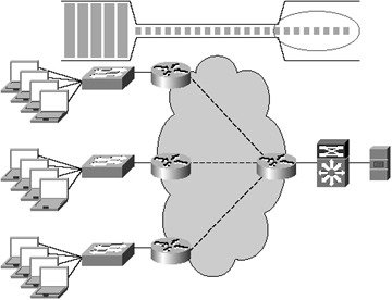
The performance challenges created by bandwidth disparity, oversubscription, and aggregation can quickly degrade application performance. Not only are each of the communicating nodes strangled because their flows are negotiated onto a lower-speed link, but the flows themselves remain strangled even when returning to a higher-capacity link, as shown in Figure 2-5. From the perspective of the server, each of the clients is only sending small amounts of data at a time (due to network oversubscription and bandwidth disparity). The overall application performance is throttled because the server can then only respond to the requests as they are being received.
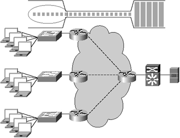
When the server responds to the client, the same challenges are encountered, as shown in Figure 2-6. Potentially large amounts of data can be sent from the server when it services a user request. This data, when set in flight, encounters the neighboring router, which is managing the bandwidth disparity, and the data is trickled over the network based on the capacity available to the flow. From the perspective of the client, the server is only sending small amounts of data at a time (due to network oversubscription and bandwidth disparity).
The prior examples assume a perfect world where everything works as advertised and overhead is unheard of. The reality is that application protocols add overhead to message exchanges. Transport protocols add overhead in the form of segmenting, window management, and acknowledgment for guaranteed delivery. Network and data link protocols add overhead due to packetization and framing. Each of these consumes a noticeable amount of network capacity and can be classified as control information that only serves the purpose of helping data reach the distant node, reassembling data in the correct order, and informing the application on the distant node of the process that is being attempted.
This process of exchanging application data using a transport protocol over an internetwork with potentially many segments between communicating nodes directly follows the Open System Interconnection (OSI) reference model, which is outlined in Table 2-1.
Table 2-1. Open System Interconnection Reference Model
Description | |
|---|---|
Application (7) | Provides services directly to user applications. Because of the potentially wide variety of applications, this layer must provide a wealth of services, including establishing privacy mechanisms, authenticating the intended communication partners, and determining if adequate resources are present. This layer is also responsible for the client-to-server or peer-to-peer exchanges of information that are necessary from the application perspective. |
Presentation (6) | Provides data transformation and assimilation guidelines to provide a common interface for user applications, including services such as reformatting, data compression, and encryption. The presentation layer is responsible for the structure and format of data being exchanged between two application processes. |
Session (5) | Establishes, manages, and maintains connections between two nodes and manages the interaction between end systems. The session layer is not always implemented but is commonly helpful in environments where structured communications are necessary, including web conferencing, collaboration over the network, and environments that leverage remote procedure calls or named pipes. |
Transport (4) | Insulates the upper three layers—5–7— (commonly bundled together as an “application layer”) from the complexities of Layers 1–3 (commonly bundled together as a “network layer”). The transport layer is responsible for the exchange of datagrams between nodes over an internetwork. The transport protocol commonly implements either a connection-oriented transmission protocol that provides guaranteed delivery (such as TCP) or a connectionless protocol that does not provide guaranteed delivery (UDP). |
Network (3) | Establishes, maintains, and terminates network connections. Among other functions, standards define how data routing and relaying are handled. Packets are exchanged between two nodes that are attached to an internetwork when each has an internetwork address that can be reached directly or through a routed infrastructure. |
Data link (2) | Ensures the reliability of the physical link established at Layer 1. Standards define how data frames are recognized and provide necessary flow control and error handling at the frame level. Frames are exchanged between two nodes that are on a common shared medium. |
Physical (1) | Controls transmission of the raw bitstream over the transmission medium. Standards for this layer define such parameters as the amount of signal voltage swing, the duration of voltages (bits), and so on. |
The application reads and writes blocks of data to a socket interface, which abstracts the transport protocol itself from the application. The blocks of data vary in size based on the application and the amount of memory allocated to the socket buffers. Application data blocks are generally 1 KB to 64 KB in size, and in some cases can be larger or smaller. Notice that an application data block is measured in bytes and not bits, as from the perspective of an application it is simply reading or writing block data to or from a buffer in memory.
The transport protocol is then responsible for draining data from the socket buffer into the network layer. When the data is written to the socket buffer by the application layer, the socket interacts with the transport protocol to segment data into datagrams. These datagrams are sized with the knowledge of the network transmission capacity (based on a search, discovery, or predefined parameter if using rate-based transmission protocols). For connection-oriented transmission protocols such as TCP, control information such as source and destination ports is attached along with other information, including cyclic redundancy check (CRC)/checksum information, segment length, offset, sequence number, acknowledgment number, and other flags. Most other transport protocols, reliable or not, provide additional data that helps to identify the application process on the local and distant nodes, along with checksum information to provide some means of guaranteeing data integrity and correctness, as well as other flow-control parameters.
The transport protocol manages both the drainage of data written to socket buffers into segments of data exchanged on the network and the extraction of data received from the network into socket buffers to be read by a local application. When data has been read from the socket buffer and processed by TCP (it is ready to be handled by the network layer), it is packetized by the network protocol (in this case, IP), where a header and trailer are added denoting the source and destination network address on the internetwork. Other information might be included such as version, header length, type of service, fragment identification, header checksums, protocol, options, and other flags.
The network protocol (generally IP) then sends the packet to be framed at the data link layer (generally Ethernet), where yet another header and trailer are added denoting the source and destination address of the next adjacent recipient on the subnet (router) and other flags. Each of these layers commonly adds checksum or CRC data to ensure correctness of data.
Figure 2-7 shows the overhead associated with application data traversing the OSI model.
When the distant node receives the packets, the reverse process begins in order to reassemble the application data block. In many cases, as much as 20 percent or more of network bandwidth can be consumed by forwarding, routing, segmentation, and delivery guarantee-related overheads. To put it simply, the WAN, which introduces a massive bandwidth disparity, coupled with the overhead just described in this section, is not an environment conducive to high levels of application performance.
Historically, many IT organizations have simply added bandwidth capacity to the network to enable higher levels of application performance. In modern-day networks where bandwidth capacities are exponentially higher than those of the past, extra bandwidth might still erroneously be seen as the end-all fix for application performance woes. The metrics of the network have largely changed, and in many cases, the bottleneck to application performance has been shifted from the amount of bandwidth available in a network. Other aspects of the network must now also be examined to fully understand where barriers to application performance lie. Latency is another aspect that must be carefully examined.
Latency is the period of apparent inactivity between the time the stimulus is presented and the moment a response occurs, which translated to network terminology means the amount of time necessary to transmit information from one node to the other across an internetwork. Latency can be examined in one of two ways:
One-way latency, or delay, is the amount of time it takes for data to be received by a recipient once the data leaves a transmitting node.
Roundtrip latency, which is far more complex and involves a larger degree of layers in the communications hierarchy, is the amount of time it takes not only for data to be received by a recipient once the data leaves a transmitting node, but also the amount of time it takes for the transmitting node to receive a response from the recipient.
Given that the focus of this book is directly related to application performance over the network, this book focuses on the components that impact roundtrip latency.
Communication between nodes on an internetwork involves multiple contiguous layers in a hierarchy. Each of these layers presents its own unique challenges in terms of latency, because they each incur some amount of delay in moving information from node to node. Many of these layers add only trivial amounts of latency, whereas others add significant amounts of latency. Referring to the previous section on bandwidth, you see that application data must traverse through the following:
A presentation layer, which defines how the data should be structured for the recipient
A session layer (for some session-based protocols), which defines a logical channel between nodes
A transport layer, which manages the delivery of data from one application process to another through an internetwork, and segmentation of data to enable adaptation for network transmission
A network layer, which provides global addressing for nodes on the internetwork and packetization of data for delivery
A data link layer, which provides framing and transmits data from node to node along the network path
A physical layer, which translates framed data to a serial or parallel sequence of electronic pulses or lightwaves according to the properties of the physical transmission media
Many of these processes are handled at high speeds within the initiating and receiving nodes. For instance, translation of framed data to the “wire” is handled in hardware by the network interface card (NIC). Packetization (network layer) and segmentation (transport layer) are largely handled by the NIC in conjunction with the CPU and memory subsystem of the node. Application data, its presentation, and the management of session control (if present) are also handled largely by the CPU and memory subsystem of the node. These processes, with the exception of managing guaranteed delivery, tend to take an amount of time measured in microseconds, which does not yield a significant amount of delay.
In some cases, systems such as servers that provide services for a large number of connected application peers and handle transmission of large volumes of application data might encounter performance degradation or scalability loss caused by the management of the transmission protocol, in most cases TCP. With TCP and any other transport protocol that provides connection-oriented service with guaranteed delivery, some amount of overhead is encountered. This overhead can be very small or very large, depending on several factors, including application workload, network characteristics, congestion, packet loss, delay, and the number of peers that data is being exchanged with.
For each connection that is established, system resources must be allocated for that connection. Memory is allocated to provide a buffer pool for data that is being transmitted and data that is being received. The CPU subsystem is used to calculate sliding window positions, manage acknowledgments, and determine if retransmission of data is necessary due to missing data or bad checksums.
For a system that is handling only a handful of TCP connections, such as a client workstation, this overhead is minimal and usually does not noticeably impact overall application performance. For a system that is handling a large number of TCP connections and moving large sums of application data, the overhead of managing the transport protocol can be quite significant, to the tune of consuming the majority of the resources in the memory and CPU subsystems due to buffer space allocation and context switching.
To fully understand why TCP can be considered a resource-intensive transport protocol and how this translates to latency, let’s examine TCP in detail.
First, TCP is a transport protocol that provides connection-oriented service, which means a connection must be established between two nodes that wish to exchange application data. This connection, or socket, identifies ports, or logical identifiers, that correlate directly to an application process running on each of the two nodes. In this way, a client will have a port assigned to the application that wishes to exchange data, and the server that the client is communicating with will also have a port. Once the connection is established, application processes on the two connected nodes are then able to exchange application data across the socket.
The process of establishing the connection involves the exchange of control data through the use of TCP connection establishment messages, including the following:
TCP SYN: The TCP SYN, or synchronize, message is sent from the node originating a request to a node to which it would like to establish a connection. The SYN message contains the local application process port identifier and the desired remote application process port. The SYN message also includes other variables, such as sequence number, window size, checksum, and options. Such TCP options include the Maximum Segment Size (MSS), window scaling, and Selective Acknowledgement (SACK). This message notifies the recipient that someone would like to establish a connection.
TCP ACK: The TCP ACK, or acknowledge, message is sent in return from the receiving peer to the originating peer. This message acknowledges the originating peer’s request to connect and provides an acknowledgment number. From here on, the sequence number and acknowledgment number are used to control delivery of data.
TCP connections are bidirectional in that the two nodes are able to exchange information in either direction. That is, the originating peer should be able to send data to the receiving peer, and the receiving peer should be able to send data to the originating peer. Given that information needs to be exchanged in both directions, a SYN must be sent from the originating peer to the receiving peer, and an ACK must be sent from the receiving peer to the originating peer. To facilitate transmission of data in the reverse direction, the receiving peer will also send a SYN to the originating peer, causing the originating peer to respond with an ACK.
The SYN and ACK messages that are exchanged between peers are flags within a TCP datagram, and TCP allows for multiple flags to be set concurrently. As such, the process of exchanging SYN and ACK messages to establish a connection is simplified, because the receiving peer can effectively establish a connection in the reverse path while acknowledging the connection request in the forward path.
Given that the SYN and ACK flags can be set together within a TCP datagram, you will see a message called a SYN/ACK, which is the receiving node acknowledging the connection request and also attempting connection in the reverse path. This is used in favor of exchanging separate SYN and ACK control datagrams in the reverse direction.
Figure 2-8 illustrates the process of establishing a TCP connection.
Now that a connection has been established, application processes can begin exchanging data. Data exchanged between application processes on two communicating nodes will use this connection as a means of guaranteeing delivery of data between the two nodes, as illustrated in Figure 2-9.
Second, TCP provides guaranteed delivery. Providing guarantees for delivery involves not only acknowledgment upon successful receipt of data, but also verification that the data has not changed in flight (through checksum verification), reordering of data if delivered out of order (through sequence number analysis), and also flow control (windowing) to ensure that data is being transmitted at a rate that the recipient (and the network) can handle.
Each node must allocate a certain amount of memory to a transmit buffer and a receive buffer for any sockets that are connected. These buffers are used to queue data for transmission from a local application process, and queue data received from the network until the local application process is able to read it from the buffer. Figure 2-10 shows how TCP acts as an intermediary between applications and the network and manages movement of data among data buffers while managing the connection between application processes.
Each exchange of data between two connected peers involves a 32-bit sequence number (coordinating position within the data stream and identifying which data has been previously sent) and, if the ACK flag is set, an acknowledgment number (defining which segments have been received and which sequence is expected next). An ACK message acknowledges that all segments up to the specified acknowledgment number have been received.
For each segment that is transmitted by an originating node, a duplicate copy of the segment is placed in a retransmission queue and a retransmission timer is started. If the retransmission timer set for that segment expires before an acknowledgment number that includes the segment is received from the recipient, the segment is retransmitted from the retransmission queue. If an acknowledgment number is received that includes the segment before the retransmission timer expires, the segment has been delivered successfully and is removed from the retransmission queue. If the timer set for the segment continues to expire, an error condition is generated resulting in termination of the connection. Acknowledgment is generated when the data has passed checksum verification and is stored in the TCP receive buffer, waiting to be pulled out by the application process.
Each exchange of data between two connected peers involves a 16-bit checksum number. The recipient uses the checksum to verify that the data received is identical to the data sent by the originating node. If the checksum verification fails, the segment is discarded and not acknowledged, thereby causing the originating node to retransmit the segment. A checksum is not fail-safe, however, but does serve to provide a substantial level of probability that the data being received is in fact identical to the data transmitted by the sender.
The TCP checksum is not the only means of validating data correctness. The IPv4 header provides a header checksum, and Ethernet provides a CRC. As mentioned previously, these do not provide a fail-safe guarantee that the data received is correct but do minimize the probability that data received is incorrect substantially.
As each segment is received, the sequence number is examined and the data is placed in the correct order relative to the other segments. In this way, data can be received out of order, and TCP will reorder the data to ensure that it is consistent with the series in which the originating node transmitted the data. Most connection-oriented transmission protocols support some form of sequencing to compensate for situations where data has been received out of order. Many connectionless transmission protocols, however, do not, and thus might not even have the knowledge necessary to understand the sequencing of the data being sent or received.
Flow control is the process of ensuring that data is sent at a rate that the recipient and the network are able to sustain. From the perspective of an end node participating in a conversation, flow control consists of what is known as the sliding window. The sliding window is a block of data referenced by pointers that indicates what data has been sent and is unacknowledged (which also resides in the retransmission buffer in case of failure), and what data has not yet been sent but resides in the socket buffer and the recipient is able to receive based on available capacity within the window.
As a recipient receives data from the network, the data is placed in the socket buffer and TCP sends acknowledgments for that data, thereby advancing the window (the sliding window). When the window slides, pointers are shifted to represent a higher range of bytes, indicating that data represented by lower pointer values has already been successfully sent and written to the recipient socket buffer. Assuming more data can be transmitted (recipient is able to receive), the data will be transmitted.
The sliding window controls the value of the window size, or win, parameter within TCP, which dictates how much data the recipient is able to receive at any point in time. As data is acknowledged, the win value can be increased, thereby notifying the sender that more data can be sent. Unlike the acknowledgment number, which is incremented when data has been successfully received by a receiving node and written to the recipient socket buffer, the win value is not incremented until the receiving node’s application process actually extracts data from the socket buffer, thereby relieving capacity within the socket buffer.
The effect of a zero win value is to stop the transmitter from sending data, a situation encountered commonly when a recipient’s socket buffer is completely full. As a result, the receiver is unable to accept any more data until the receiver application extracts data from the socket buffer successfully, thereby freeing up capacity to receive more data. The network aspects of flow control are examined in the later section, “Throughput.” Figure 2-11 shows an example of how TCP windows are managed.
The connection-oriented, guaranteed-delivery nature of TCP causes TCP to consume significant resources and add latency that can impair application performance. Each connection established requires some amount of CPU and memory resources on the communicating nodes. Connection establishment requires the exchange of control data across the network, which incurs transmission and network delays. Managing flow control, acknowledging data, and retransmitting lost or failed data incur transmission and network delays.
How do other transport protocols fare compared to TCP? Other transport protocols, such as UDP, are connectionless and provide no means for guaranteed delivery. These transport protocols rely on other mechanisms to provide guaranteed delivery, reordering, and retransmission. In many cases, these mechanisms are built directly into the application that is using the transport protocol.
While transport protocols such as UDP do not directly have the overhead found in TCP, these overhead-inducing components are often encountered in other areas, such as the application layer. Furthermore, with a transport protocol that does not have its own network-sensitive mechanism for flow control, such transport protocols operate under the management of an application and will consume as much network capacity as possible to satisfy the application’s needs with no consideration given to the network itself.
Although the transport layer can certainly add incremental amounts of latency due to connection management, retransmission, guaranteed delivery, and flow control, clearly the largest impact from the perspective of latency comes from physics. Put simply, every network connection between two nodes spans some distance, and sending data across any distance takes some amount of time.
In a complex internetwork, a network connection might be between two nodes but span many intermediary devices over tens, hundreds, thousands, or tens of thousands of miles. This delay, called propagation delay, is defined as the amount of time taken by a signal when traversing a medium. This propagation delay is directly related to two components:
Physical separation: The distance between two nodes
Propagation velocity: The speed at which data can be moved
The maximum propagation velocity found in networks today is approximately two-thirds the speed of light (the speed of light is 3 × 10⁸ m/sec, therefore the maximum propagation velocity found in networks today is approximately 2 × 10⁸ m/sec). The propagation delay, then, is the physical separation (in meters) divided by the propagation delay of the link (2 × 10⁸ m/sec).
For a connection that spans 1 m, information can be transferred in one direction in approximately 5 nanoseconds (ns). This connection presents a roundtrip latency of approximately 10 ns.
For a connection that spans 1000 miles (1 mile = 1600 m), or 1.6 million meters, information can be transferred in one direction in approximately 8 ms. This connection presents a roundtrip latency of approximately 16 ms.
For a satellite connection that spans 50,000 miles (1 mile = 1600 m), or 80 million meters, information can be transferred in one direction in approximately 400 ms. This connection presents a roundtrip latency of approximately 800 ms.
These latency numbers are relative only to the amount of time spent on the network transmission medium and do not account for other very important factors such as serialization delays, processing delays, forwarding delays, or other delays.
Serialization delays are the amount of time it takes for a device to extract data from one queue and packetize that data onto the next network for transmission. Serialization delay is directly related to the network medium, interface speed, and size of the frame being serviced. For higher-speed networks, serialization delay might be negligible, but in lower-speed networks, serialization delay can be significant. Serialization delay can be calculated as the size of the data being transferred (in bits) divided by the speed of the link (in bits). For instance, to place 100 bytes of data (roughly 800 bits) onto a 128-kbps link, serialization delay would be 6.25 ms. To place 100 bytes of data onto a 1-Gbps link, serialization delay would be 100 ns.
Processing delays are the amount of time spent within a network node such as a router, switch, firewall, or accelerator, determining how to handle a piece of data based on preconfigured or dynamic policy. For instance, on an uncongested router, a piece of data can be compared against a basic access list in under 1 millisecond (ms). On a congested router, however, the same operation might take 5 to 10 ms.
The forwarding architecture of the network node impacts processing delay as well. For instance, store-and-forward devices will wait until the entire packet is received before making a forwarding decision. Devices that perform cut-through forwarding will make a decision after the header is received.
Forwarding delays are the amount of time spent determining where to forward a piece of data. With modern routers and switches that leverage dedicated hardware for forwarding, a piece of data may move through the device in under 1 ms. Under load, this may increase to 3 to 5 ms.
The sum of all of these components (physics, transport protocols, application protocols, congestion) adds up to the amount of perceived network latency. For a direct node-to-node connection over a switch, network latency is generally so small that it does not need to be accounted for. If that same switch is under heavy load, network latency may be significantly higher, but likely not enough to be noticeable. For a node-to-node connection over a complex, hierarchal network, latency can become quite significant, as illustrated in Figure 2-12.
This latency accounts for the no-load network components in the path between two nodes that wish to exchange application data. In scenarios where intermediary devices are encountering severe levels of congestion, perceived latency can be dramatically higher.
With this in mind, you need to ask, “Why is latency the silent killer of application performance?” The reason is quite simple. Each message that must be exchanged between two nodes that have an established connection must traverse this heavily latent network. In the preceding example where the perceived roundtrip network latency was 48 ms, we must now account for the number of messages that are exchanged across this network to handle transport protocol management and application message transfer.
In terms of transport protocol management, TCP requires connection management due to its nature as a connection-oriented, guaranteed-delivery transport protocol. Establishing a connection requires 1.5 round trips across the network. Segment exchanges require round trips across the network. Retransmissions require round trips across the network. In short, every TCP segment sent across the network will take an amount of time equivalent to the current network delay to propagate.
To make matters worse, many applications use protocols that not only dictate how data should be exchanged, but also include semantics to control access, manage state, or structure the exchange of data between two nodes. Such application protocols are considered “chatty” or said to “play network ping-pong” or “ricochet” because of how many messages must actually be exchanged before a hint of usable application data is exchanged between the two nodes.
Take HTTP, for example, as illustrated in Figure 2-13. In a very basic web page access scenario, a TCP connection must first be established. Once established, the user’s browser then requests the container page for the website being viewed using a GET request. When the container page is fully transferred, the browser builds the structure of the page in the display window and proceeds to fetch each of the embedded objects listed in the container page. Oftentimes, this is done over one or two concurrent TCP connections using serialized requests for objects. That is, when one object is requested, the next object cannot be requested until the previous object has been completely received. If the browser is using a pair of TCP connections for object fetching, two objects can be transferred to the browser at any given time, one per connection. For a website with a large number of objects, this means that multiple GET requests and object transfers must traverse the network.
In this example, assuming no network congestion, packet loss, or retransmission, and that all objects are transferable within the confines of a single packet, a 100-object website using two connections for object fetching over a 100-ms network (200-ms roundtrip latency) would require the following:
1.5 × 200 ms for TCP connection 1 setup (300 ms)
1 × 200 ms for the fetch of the container page (200 ms)
1.5 × 200 ms × 2 for TCP connections 2 and 3 setup (600 ms)
50 × 200 ms for the fetch of 100 objects using two connections (10 sec)
The rendering of this website would take approximately 11 seconds to complete due to the latency of the application protocol being used. This does not account for network congestion, server response time, client response time, or many other very important factors. In some cases, based on application design or server configuration, these objects may already be cached on the client but require validation by the application protocol. This leads to additional inefficiency as objects that are stored locally are verified as valid and usable.
HTTP is not the only protocol that behaves this way. Many other application protocols are actually far worse. Other “ping-pong” application protocols that require extensive messaging before useful application data is ever transmitted include the following:
Common Internet File System (CIFS): Used for Windows file-sharing environments
Network File System (NFS): Used for UNIX file-sharing environments
Remote Procedure Call (RPC): Used extensively by applications that rely on a session-layer, including e-mail and collaboration applications such as Microsoft Exchange
More details on application protocol inefficiencies will be discussed later in this chapter in the “Application Protocols” section.
The previous sections have examined network capacity (bandwidth) and latency as network characteristics that deteriorate application performance over the WAN. The third most common performance limiter is throughput. Throughput, or the net effective data transfer rate, is impacted by the following characteristics of any internetwork:
Capacity: The minimum and maximum amount of available bandwidth within the internetwork between two connected nodes
Latency: The distance between two connected nodes and the amount of time taken to exchange data
Packet loss: The percentage of packets that are lost in transit due to oversubscription, congestion, or other network events
Network capacity is the easiest challenge to identify and eliminate because it relates to application performance over the network. With network capacity, the amount of throughput an application can utilize will never exceed the available capacity of the smallest intermediary hop in the network. For instance, assume a remote branch office has Gigabit Ethernet connectivity to each of the workstations in the office, and the router connects to a T1 line (1.544 Mbps). On the other end of the T1 line, the WAN router connects the corporate headquarters network to all of the remote sites. Within the corporate headquarters network, each server is connected via Gigabit Ethernet. Although the client in the branch office and the server in the corporate headquarters network are both connected by way of Gigabit Ethernet, the fact remains that they are separated by a T1 line, which is the weakest link in the chain.
In this scenario, when user traffic destined to the server reaches the network element that is managing the bandwidth disparity (that is, the router), congestion occurs, followed by backpressure, which results in dramatically slower application performance, as shown in Figures 2-5 and 2-6 earlier in the chapter. The same happens in the reverse direction when the server returns data back to the client. In this simple case, adding WAN bandwidth may improve overall user throughput, assuming the available bandwidth is indeed the limiting factor.
For congested networks, another way to overcome the challenge is to examine traffic flows that are consuming network resources (classification), assigning them a relative business priority (prioritization), and employing quality of service (QoS) to provision network resources for those flows according to business priority.
Network capacity is not, however, the limiting factor in many cases. In some situations, clients and servers may be attached to their respective LAN via Gigabit Ethernet and separated via a T1, and upgrading from a T1 to a T3 provides little if no improvement in throughput. How can it be that an organization can increase its bandwidth capacity in the WAN by an order of magnitude without providing a noticeable improvement in application performance? The answer is that the transport protocol itself may be causing a throughput limitation.
From earlier sections, you know that TCP consumes system resources on each communicating node, and that there is some overhead associated with TCP due to transmit and receive buffer management, flow control, data reordering, checksum verification, and retransmissions. With this in mind, you can expect that you will pay a performance penalty if you are to use a transport protocol that guarantees reliable delivery of data. However, there are larger issues that plague TCP, which can decrease throughput of an application over a WAN.
First, TCP does not require a node to have explicit understanding of the network that exists between itself and a peer. In this way, TCP abstracts the networking layer from the application layer. With a built-in mechanism for initially detecting network capacity (that is, TCP slow start), TCP is safe to use in almost any network environment. This mechanism, however, was designed over 20 years ago when network capacity was minimal (think 300-bps line). Although extensions to TCP improve its behavior, only some have become mainstream. The remaining extensions are largely unused.
Second, TCP not only has a built-in mechanism for detecting initial network capacity but also has a mechanism for adapting to changes in the network. With this mechanism, called congestion avoidance, TCP is able to dynamically change the throughput characteristics of a connection when a congestion event (that is, packet loss) is encountered. The way TCP adapts to these changes is based on the algorithms designed over 20 years ago, which provide safety and fairness, but is lacking in terms of ensuring high levels of application performance over the WAN. At the time of TCP’s inception, the most network-intensive application was likely Telnet, which hardly puts a strain on even the smallest of network connections.
To summarize these two mechanisms of TCP—slow start and congestion avoidance—that hinder application performance over the WAN, remember that slow start helps TCP identify the available network capacity and that congestion avoidance helps TCP adapt to changes in the network, that is, packet loss, congestion, or variance in available bandwidth. Each mechanism can directly impact application throughput in WAN environments, as discussed in the following sections.
What is TCP slow start and how does it impact application throughput in WAN environments? TCP slow start allows TCP to identify the amount of network capacity available to a connection and has a direct impact on the throughput of the connection. When a connection has first been established, TCP slow start allows the connection to send only a small quantity of segments (generally, up to 1460 bytes per segment) until it has a history of these segments being acknowledged properly.
The rate at which TCP allows applications to send additional segments is exponential, starting from a point of allowing a connection to send only one segment until the acknowledgment of that segment is received. This variable that is constantly changing as segments are acknowledged is called the congestion window, or cwnd.
When a packet-loss event is encountered during the TCP slow start phase, TCP considers this the moment that the network capacity has been reached. At this point, TCP decreases the congestion window by 50 percent and then sends the connection into congestion avoidance mode, as shown in Figure 2-14.
The congestion window, along with the maximum window size, determines the maximum amount of data that can be in flight for a connection at any given time. In fact, the lesser of the two (congestion window vs. maximum window size) is considered the maximum amount of data that can be in flight, unacknowledged, at any given time. For instance, if a packet-loss event is never encountered, the connection will not exit the TCP slow start phase. In such a scenario, the amount of network capacity is likely very high and congestion is nearly nonexistent. With such a situation, the TCP throughput will be limited by the maximum window size or by other variables such as capacity in the send and receive buffers and the latency of the network (how quickly data can be acknowledged).
TCP slow start hinders application throughput by starving connections of precious bandwidth at the beginning of their life. Many application transactions could occur in a relatively small number of roundtrip exchanges, assuming they had available bandwidth to do so. While TCP is busy trying to determine network capacity, application data is waiting to be transmitted, potentially delaying the entire application. In this way, TCP slow start extends the number of roundtrip exchanges that are necessary to complete a potentially arbitrary operation at the beginning of a connection.
The other mechanism of TCP that can have a negative impact on application performance is congestion avoidance. TCP congestion avoidance allows a TCP connection that has successfully completed slow start to adapt to changes in network conditions, such as packet-loss or congestion events, while continuing to safely search for available network capacity.
Whereas TCP slow start employs an exponential search for available network bandwidth, TCP congestion avoidance employs a linear search for available network bandwidth. For every successfully acknowledged segment during TCP congestion avoidance, TCP allows the connection to increment its congestion window value by one additional segment. This means that a larger amount of bandwidth can be consumed as the age of the connection increases, assuming the congestion window value is less than the value of the maximum window size. When packet loss is encountered during the congestion avoidance phase, TCP again decreases the congestion window, and potential throughput, by 50 percent. With TCP congestion avoidance, TCP slowly increases its congestion window, and consequently throughput, over time, and encounters substantial throughput declines when packet loss is encountered, as shown in Figure 2-15.
TCP congestion avoidance is not an issue on some networks, but on others it can have a sizeable impact on application performance. For networks that are considered to be “long and fat,” or “LFNs” (also called elephants), TCP congestion avoidance can be a challenge to ensuring consistently high levels of network utilization after loss is encountered. An LFN is a network that has a large amount of available network capacity and spans a great distance. These LFNs are generally multiple megabits in capacity but tens or hundreds of milliseconds in latency. From the perspective of TCP’s congestion avoidance algorithm, it can take quite some time for an acknowledgment to be received indicating to TCP that the connection could increase its throughput slightly. Coupled with the rate at which TCP increases throughput (one segment increase per successful round trip), it could take hours to return to maximum link capacity on an LFN.
As mentioned in the previous section, a node’s ability to drive application throughput for a TCP-based application is largely dependent on two factors: congestion window and maximum window size. The maximum window size plays an important role in application throughput in environments where the WAN is an LFN. By definition, an LFN has a large capacity and spans a great distance. An LFN can potentially carry a large amount of data in flight at any given time. This amount of network storage capacity, the amount of data that can be in flight over a link at any given time, is called the bandwidth delay product (BDP) and defines the amount of data that the network can hold.
The BDP is calculated by multiplying the bandwidth (in bytes) by the delay (round trip). For instance, a T1 line (1.544 Mbps = 190 KBps; note that lowercase b is used for bits whereas uppercase B is used for bytes) with 100 ms of delay has a BDP of approximately 19 KB, meaning only 19 KB of data can be in flight on this circuit at any given time. An OC3 line (155 Mbps, 19 MBps) with 100 ms, however, has a BDP of approximately 1.9 MB. As you can see, as bandwidth and delay increase, the capacity of the network increases.
The BDP of the network is relevant only when the nodes using the network do not support a maximum window size (MWS) that is larger than the BDP itself. The client’s maximum amount of outstanding data on the network can never exceed the smaller of either cwnd or MWS. If the BDP of the network is larger than both of these values, then there is capacity available in the network that the communicating node cannot leverage, as shown in Figure 2-16. Even if cwnd were to exceed the MWS, it would not matter, because the smaller of the two determines the maximum amount of outstanding data on the wire.
Bandwidth, latency, packet loss, and throughput intertwine with one another to determine maximum levels of application throughput on a given network. The previous sections examined the factors that directly impact application performance on the network. The next section examines other factors outside of the network infrastructure itself, including hardware considerations, software considerations, and application considerations, that can also have a significant impact on application performance and stability.
The performance of an application is constantly impacted by the barriers and limitations of the protocols that support the given application and the network that resides between the communicating nodes. Just because an application performs well in a lab does not always mean it will perform well in a real-world environment.
As discussed earlier in this chapter, protocols react poorly when introduced to WAN conditions such as latency, bandwidth, congestion, and packet loss. Additional factors impact application performance, such as how the common protocols consume available network bandwidth and how traffic is transferred between devices. Furthermore, other application performance barriers can be present in the endpoints themselves, from something as basic as the network card to something as complex as the block size configured for a local file system.
Network latency is generally measured in milliseconds and is the delta between the time a packet leaves an originating node and the time the recipient begins to receive the packet. Several components exist that have a negative impact on perceived network latency.
Hardware components such as routers, switches, firewalls, and any other inline devices add to the amount of latency perceived by the packet, because each device applies some level of logic or forwarding. As discussed in the previous section, network characteristics such as bandwidth, packet loss, congestion, and latency all have an impact on the ability of an application to provide high levels of throughput.
Protocols that are used by applications may have been designed for LAN environments and simply do not perform well over the WAN, not because of poor application or protocol design, but simply because the WAN was not considered a use case or requirement for the protocol at the time. This section examines a few protocols and their behavior in a WAN environment, including CIFS, HTTP, NFS, and MAPI.
CIFS sessions between a client and file server can be used for many functions, including remote drive mapping, simple file copy operations, or interactive file access. CIFS operations perform very well in a LAN environment. However, given that CIFS was designed to emulate the control aspects of a shared local file system via a network interface, it requires a high degree of control and status message exchanges prior to and during the exchange of useful data. This overhead, which is really due to how robust the protocol is, can be a barrier to application performance as latency increases.
As an example, accessing a 1.5-MB file over the network that resides on a Windows file server requires well over 1000 messages to be exchanged between the client and the server. This is directly related to the fact that CIFS requires the user to be authenticated and authorized, the file needs to be found within the directory structure, information about the file needs to be queried, the user permissions need to be verified, file open requests must be managed, lock requests must be handled, and data must be read from various points within the file (most likely noncontiguous sections).
CIFS is a protocol that has a high degree of application layer chatter; that is, a large number of messages must be exchanged to accomplish an arbitrary task. With protocols such as CIFS that are chatty, as latency increases, performance decreases. The combination of chatty applications and high-latency networks becomes a significant obstacle to performance in WAN environments because a large number of messages that are sent in a serial fashion (one at a time) must each traverse a high-latency network.
Although TCP/IP is a reliable transport mechanism for CIFS to ride on top of, latency that is introduced in the network will have a greater impact on CIFS performance, because the CIFS protocol is providing, through the network as opposed to being wholly contained within a computer, all of the semantics that a local file system would provide.
CIFS does support some built-in optimization techniques through message batching and opportunistic locks, which includes local caching, read-ahead, and write-behind. These optimizations are meant to grant a client the authority necessary to manage his own state based on the information provided by the server. In essence, the server will notify the user that they are the only user working with a particular object. In this way, the CIFS redirector, which is responsible for transmission of CIFS messages over the network, can respond to its own requests to provide the client with higher levels of performance while offloading the server. Although these techniques do provide value in that fewer messages must be handled by the origin server, the value in a WAN environment is nullified due to the extreme amounts of latency that exist in the network.
For Internet traffic that uses HTTP as a transfer mechanism, several factors contribute to latency and the perception of latency, including the following:
Throughput of the connection between the client and server
The speed of the client and server hosts themselves
The complexity of the data that must be processed prior to display by the client
Intranet web traffic is generally much more dynamic than traditional client/server traffic, and Internet traffic today is much more dynamic than it was 10 years ago. With the introduction of Java and other frameworks such as Microsoft’s .NET, the client browser is empowered to provide a greater degree of flexibility and much more robust user experience.
Along with the capabilities provided by such frameworks, the browser is also required to process and render a larger amount of information, which may also increase the burden on the network. Although Internet browsers have matured to include functions such as local caches, which help mitigate the transmission of locally stored objects that have been previously accessed, the browser still cannot address many of the factors that contribute to the perception of latency by the user.
For objects embedded within a web page, the browser may be required to establish additional TCP connections to transfer them. Each TCP connection is subject to the roundtrip latency that natively exists between the client and server in the network, and also causes resource utilization increases as memory is allocated to the connection. Negatively adding to an already challenged protocol, the average Internet web page is populated with a significant number of small objects, increasing the number of TCP connections required when accessing the web page to be browsed and the number of roundtrip exchanges required to fetch these embedded objects.
In a network environment with several users located in a remote branch sharing a common WAN link, browser caching aids in improving the overall performance. Browser caching does not, however, address the limitations created by the fact that every user must request his own copy of content at least once because he is not sharing a common repository. Compounding the number of users across a limited-bandwidth WAN link adds latency to their browsers’ ability to receive requested HTTP data. Application response times increase, and network performance declines predictably.
The most common browser, Microsoft Internet Explorer, opens two TCP connections by default. Though HTTP 1.1 supports pipelining to allow multiple simultaneous requests to be in process, it is not widely implemented. As such, HTTP requests must be serially processed over the two available TCP connections.
A typical web page is composed of a dynamic object or container page and many static objects of varying size. The dynamic object is not cached, whereas the static objects may be locally cached by the client browser cache or perhaps an intermediate public cache. In reality, even the static objects are often marked noncacheable or immediately expired because the application owner either is trying to account for every delivery or has at some point experienced problems with stale objects in web caches.
The application owner’s knee-jerk reaction was to immediately expire all objects allowing the client to cache an object but then force the client to issue an If-Modified-Since (IMS) to revalidate the objects’ freshness. In this case, a web page with 100 objects that may be cached in the client browser cache would still have to IMS 100 times over two connections, resulting in 50 round trips over the WAN. For a 100-msec RTT network, the client would have to wait 5 seconds just to revalidate while no real data is traversing the network.
By nature, HTTP does not abide by any given bandwidth limitation rules. HTTP accepts however much or little bandwidth is made available via the transport layer (TCP) and is very accepting of slow links. Consider that a web browser will operate the same if connecting to the Internet via a 2400-bps modem or a 100-Mbps Ethernet card, with the only difference being the time required to achieve the same results.
Some HTTP implementations are forgiving of network disruption as well, picking up where the previous transmission was disrupted. The lines that separate an application from the traditional browser have been blurring over the past several years, moving the browser from an informational application to the role of critical business application. Even with the evolution in role for the web browser, HTTP still abides by its unbiased acceptance of the network’s availability.
With the transition of many core business-related applications from client/server to HTTP based, some applications use client-based software components while still using HTTP as the transport mechanism. With the vast success of Java, application infrastructure can be centralized, yet, segments of the application (such as applets) can be distributed and executed on the remote user workstation via his web browser. This benefits the application and server in two ways:
The server processes less of the application.
Processor-intensive efforts can reside on the client’s workstation.
Following this model a step further, it is common for only the database entries to traverse the network and for any new Java applets to be distributed to the client as needed. The client continues to access the application via the local Java applets that are active in their browser. The applet remains available until the browser is closed or a replacement applet is served from the application server. This process works very well when the client has the Java applet loaded into the browser, but getting the initial Java applet(s) to the client consumes any bandwidth made available to HTTP during the transfer.
Many web-accessible database applications are available today and are commonly tested in a data center prior to their deployment within the corporate network. As previously shown in Chapter 1, “Strategic Information Technology Initiatives,” the testing of new applications commonly takes place within a lab and not in a network environment that mirrors a full production remote branch. If a branch location has 20 users, each requiring access to the same application, that application must traverse the shared WAN link 20 times.
Testing of applications that use an actual production branch may not test the application and WAN to their fullest capacity, that is, all users simultaneously within the branch. Some applications may load in seconds when tested in a lab with high-speed LAN links connecting the client, but when tested over a WAN link with 20 simultaneous users sharing the common WAN link, it could take 30 minutes or more for the same application to become available to all users in that branch.
Due to the forgiving nature of HTTP, the loading of the application becomes slow to the user but does not time out or fail the process of loading. Branch PCs commonly have slow access in the morning, because applications must be loaded on workstations, and other business-critical functions, such as e-mail and user authentication, traverse the network at the same time. HTTP does not care about what else is happening on the network (TCP does), as long as the requested content can eventually transfer to the client’s browser.
Many network administrators consider the FTP a “necessary evil.” Legacy applications and logging hosts commonly use FTP for simple, authenticated file transfers. FTP is viewed as a simple solution but with a potential for a major impact. Everything from the NIC of the server to the WAN link that the traffic will traverse is impacted by the manner in which FTP transfers content. FTP can disrupt the ability to pass other traffic at the same time an FTP transfer is taking place. By nature, FTP consumes as much bandwidth as possible during its transfer of content, based on what TCP is allowed to consume. FTP tends to use large data buffers, meaning it will try to leverage all of the buffer capacity that TCP can allocate to it.
Precautions exist within many operating systems and third-party applications that allow the administrator to define an upper limit to any given FTP transfer, preventing congestion situations. FTP is not fault tolerant and, by nature, is very unforgiving to disruptions. In many cases, a network disruption requires that the file be retransmitted from the beginning. Some application vendors have written client and server programs that leverage FTP as a control and data transfer protocol that allow for continuation of a failed transfer, but these mechanisms are not built into FTP as a protocol itself.
NFS, which was originally introduced by Sun Microsystems, provides a common protocol for file access between hosts. NFS provides read and write capabilities similar to CIFS, but NFS is stateless in nature whereas CIFS is extremely stateful. This means that the server requires use of idempotent operations, that is, each operation contains enough data necessary to allow the server to fulfill the request. With CIFS, the server knows the state of the client and the file and can respond to simple operations given the known state.
Since the acceptance of NFS by the Internet Engineering Task Force (IETF), vendors such as Microsoft, Novell, Apple, and Red Hat have adopted the NFS protocol and implemented a version into their server and client platforms.
Although the standards are clearly defined to implement NFS, there are currently three common versions of NFS that all have different abilities and create and react differently to latency challenges introduced on the network. NFS version 2 (NFSv2) leverages UDP as a transport layer protocol, which makes it unreliable in many network environments. Although some implementations of NFSv2 now support TCP, NFSv3 was more easily adopted due to its native support of TCP for transport.
NFS is similar to CIFS in that a physical location within a file system is made accessible via the network, and clients are able to access this shared file system as if it were local storage. NFS introduces some challenges that are similar to those of CIFS, including remote server processing delay when data is being written to the remote host, and sensitivity to network latency when data is being read from or written to a remote host.
For file transfers, NFS generally uses 8-KB blocks for both read and write actions. NFS impacts more than just the network; NFS also impacts the CPU of the server, disk throughput, and RAM. There is a direct parallel between the volume of data being transferred via NFS and the amount of server resources consumed by NFS.
Fortunately, vendors such as Sun have implemented bandwidth management functionality, allowing for NFS traffic flows to be throttled for both incoming and outgoing traffic independently of each other. If bandwidth management is not applied to NFS traffic, as with other protocols, the client application will consume as much bandwidth as allowed by the transport protocol. As network speeds become faster, file sizes will trend toward becoming larger as well. NFS has been used by applications as a transport for moving database and system backup files throughout the network, requiring that traffic management be planned in advance of implementing the NFS protocol.
The ability to control NFS traffic on the WAN will aid administrators in preventing WAN bottleneck slowdowns. Much like CIFS, if 50 users in a remote office each need a copy of the same file from the same mount point, the file must be transferred across the network at least once for each requesting user, thereby wasting precious WAN bandwidth.
MAPI provides a common message exchange format that can be leveraged in client/server and peer-to-peer applications. MAPI is commonly used as a standardized means of exchanging data over another protocol such as a Remote Procedure Call (RPC). For instance, Microsoft Exchange uses MAPI for the structuring of messages that are exchanged using remote-procedure calls (RPC). Although not all vendors’ implementation of MAPI may be the same, not to mention the use of the protocol that is carrying data (such as RPC), several applications use MAPI to dictate the way messages are exchanged.
Throughput of many client/server applications that leverage MAPI, such as Microsoft Outlook and Exchange, which use MAPI within RPC, decreases by as much as 90 percent as latency increases from 30 ms to 100 ms. As e-mail continues to become an increasingly important enterprise application, poor performance of e-mail services within the network is generally brought to the attention of network administrators faster than other poorly performing business-critical applications. The majority of this decline in application performance is directly related to bandwidth, latency, throughput, and the inefficiencies of the protocol being used to carry MAPI message exchanges.
Microsoft’s use of MAPI and RPC differs between Exchange Server 2000 and Exchange Server 2003. Traffic patterns between the two different server versions differ from the perspective of network traffic due to the introduction of cached mode in Exchange Server 2003, when used in conjunction with the matching Microsoft Outlook 2003 product. When Exchange 2003 and Outlook 2003 are combined, cached mode allows for the majority of user operations to be performed locally against a “cached copy” of the contents of the user’s storage repository on the server. In essence, cached mode allows a user to keep a local copy of his storage repository on the local PC. This local copy is used to allow operations that do not impact data integrity or correctness to be handled locally without requiring an exchange of data with the Exchange server. For instance, opening an e-mail that resides in the cached copy on the local PC does not require that the e-mail be transferred again from the Exchange server. Only in cases where updates need to be employed, where state changes, or when synchronization is necessary do the server and client actually have to communicate with one another.
E-mail vendors such as Lotus, with its Domino offering, support compression and other localization functions as well. Lotus recognizes that allowing less traffic to traverse the WAN between the client and server will improve application performance for its users.
Although compression reduces the overall volume of data that traverses the network, e-mail protocols are still very sensitive to latency and packet loss. When operating on networks that are subject to a predictable amount of traffic loss, e-mail may not function at all, making services appear as if they are offline. Most e-mail applications have a default interval of 60 seconds for synchronization between the client and server. With such offline synchronization, traffic is greatly reduced once the e-mail client has sent and received all of its messages and has synchronized the local cached copy. However, if the amount of data that needs to be synchronized to the server is large and transfer of this data extends beyond the synchronization window, it could be quite difficult for a client to catch up. Similar to file-sharing protocols, if 50 users in a remote office each received a copy of the same e-mail with the same 5-MB attachment, that 5-MB attachment would be transferred across the network once per recipient, consuming large amounts of network capacity.
The networks of today are much more stable than they were 10 years ago. As bandwidth capacity has continued to increase, so has the amount of memory and hardware capacity of the devices (routers and switches) that direct traffic on private and public networks. With this increase in network capacity and network element hardware, packet loss is far less noticeable in the enterprise network and very rare across the public Internet, primarily because the bottlenecks have shifted away from the network.
Network stability is still a key factor in today’s networks as some networks transition from Fast Ethernet (100 Mbps) to Gigabit Ethernet (1000 Mbps), or even to 10-Gigabit Ethernet (10,000 Mbps). Traffic at these speeds will traverse a router or switch that needs to accommodate not just the traffic of one client to one server, but potentially from hundreds or thousands of nodes.
Several components impact overall stability of the network, including each of the network elements (routers, switches, firewalls), wireless access points, cabling, and more. For outsourced or managed WAN environments, network stability also includes a service provider plan and its network offerings that connect the data center and remote branch location, including any optional redundancy or service level agreements (SLA).
An unreliable network has an impact on more than just the data that traverses the network. Factors that cannot be as easily monitored or calculated, such as employee morale, can cost an enterprise in ways that cannot be forecasted. Employees who depend on an unreliable network may avoid certain applications, or look to alternative methods to get a job done if they do not feel that they can efficiently or, more importantly, reliably perform their required daily tasks. In some cases, the employees may just refuse to do their jobs, because they do not feel that they have adequate tools available to complete their assigned tasks. As mentioned in Chapter 1, sometimes the application is to blame for poor performance, and in some cases the network is to blame. In this case, the network is to blame if stability is impacted to the point that users cannot get to the tools they need to be productive and drive revenue.
As an example, consider how your mobile wireless provider’s network impacts the usage patterns of your personal mobile phone. Your mobile phone is dependent on an accessible network to allow you to make or receive calls. In your daily travels, you will find over the course of time that certain areas have unreliable cellular coverage. During your travels through those areas, you will disconnect from the cellular network either intentionally prior to the service disruption or unintentionally when you unknowingly enter the poor service area. Data networks and applications share many similarities. If your daily responsibilities call for you to access several applications, one of which has extremely poor performance, you will approach the usage of that one application differently than you do the others. If that one application resides in a data center that is a long distance away over an oversubscribed and unreliable network, then both the application’s and employee’s performance will suffer.
Understanding network infrastructure and network management is the first step in venturing to assess and manage application performance over the network. If you do not know how your network is designed and implemented, you will not be in a position to effectively monitor and manage your network or the applications that use it. Take the time to understand your network topology, and be sure to become familiar with each component, including the following:
The make and model of routers, switches, firewalls, server load-balancers, and other network elements currently in use at each location.
The version of operating system and licensed features that are in use on each of the network elements.
The interface number and type, as well as any assigned IP address information of each interface and node.
The interface configuration, including speed and duplex. Interfaces should either negotiate properly with the peer device or be hard-coded to the correct configuration to ensure consistency.
Similarly, become familiar with each of the non-network components that have an impact on application performance, including these:
The make and model of client laptops, desktops, and servers
The version of operating system and the licensed features that are in use on each of these
The applications that are installed and how they are configured
Service packs, hotfixes, and device drivers that are installed
The network connectivity (speed, media, network configuration) for each of these nodes and their location within the network (campus, remote office, VPN user)
From the network and non-network information, an administrator can easily identify how his network is configured, as well as where to take action if an outage is observed.
The next step in understanding the network’s impact on application performance is to know the limits of your network. Every router, switch, network card, and cable has a capacity limit. If the limiting factor is not the speed of the interface, it could be the CPU or memory utilization of each device that the traffic must traverse.
A router or switch that is running at capacity may drop an excessive number of packets (that is, become a point of congestion). If aggregation and oversubscription are not planned appropriately, packet loss and queuing delays could have a significantly adverse effect on the performance of applications traversing that device.
Network switches are commonly designed with inherent oversubscription. For instance, a switch that supports 24 ports of 1000-Mbps traffic per port may not have an adequate backplane capacity to support 24 ports under full load. Understanding the limits of a router, switch, firewall, or other network element will help identify potential bottlenecks in the network. Adequately sizing network infrastructure components will help prevent network stability issues and better guarantee higher levels of application performance.
Several monitoring utilities exist today that allow you to monitor all aspects of a router or switch. Monitoring utilities range from simple shareware tools to monitoring and reporting systems that cost millions of dollars. The following sections describe SNMP-compliant managers and syslog.
Routers and switches that support network management and monitoring via the Simple Network Management Protocol (SNMP) should be configured to report to an SNMP-compliant manager, because this will aid in providing visibility into the overall health of each of the devices. SNMP monitoring will inform an administrator of a device that exceeds a configured threshold, generates specific warnings, or triggers alerts. If a defined threshold such as CPU utilization is exceeded, the stability of the network may be at risk due to a device that cannot support or scale beyond its current workload.
SNMP supports several functions that help secure and stabilize the monitoring information that is provided by the network routers and switches. Functions include the ability to encrypt and authenticate the requests that the router or switch must respond to.
Although SNMPv1 is the most commonly implemented version, versions 2c and 3 provide additional levels of protection that help deter network threats from snooping around the network. Table 2-2 provides a simplistic overview of SNMP version differences.
In addition to SNMP, syslog can be used to monitor system-related events, which can prove useful in many network environments. Syslog tracks just about every event that occurs on the network, depending on the level of visibility desired by the network administrator. If an application is suspect in the stability or performance of a given network, implementing syslog may help in tracking down specific suspect events. Also, depending on what information you are tracking on the network, there may be legal implications that protect the employee’s rights. Syslog will help in understanding network traffic patterns, and in a way that helps determine if there are application or network failures being observed on the network.
Many network vendors today have results of performance validation tests and may make these available to customers. This information may not be publicly available due to the sensitive nature of the data. Most vendors make this information available upon request, and understanding how each device in your network behaves will help you to know what the observed limits are and how to deploy accordingly. For example, deploying a router that cannot meet the packets per second requirement or that has insufficient resources may not scale to meet the needs of the location it connects to.
One of the most important factors in network stability is the redundancy plan. Redundancy planning and implementation can be leveraged at any place within the network, ranging from the data center application servers to the remote branch WAN connectivity or even the LAN switch. With the intelligence that exists in today’s infrastructure components, redundancy has become easier to implement. Although items such as redundant WAN connections and the associated routers can be costly, the technology exists today to allow for near-immediate failover with granular control over which applications are allowed to take advantage of the alternate WAN connectivity.
Take the time to consider the options that exist when considering redundancy in the network. Proper planning is the key to providing network access that is scalable, reliable, and stable for the remote user. In most cases, the cost of downtime is far greater than the cost of redundancy.
The client and server also are large factors in network stability and application performance, starting with the connection point to the network, the NIC. For all devices, if the client or server network connection is not stable (because of improper device drivers, faulty network cards, bad cables, or a poorly implemented or misconfigured TCP/IP stack, for example), then the network will appear to lack stability and application performance will suffer.
The device driver selected by the operating system may not always be the most appropriate, accurate, or current. Ensuring that servers, client workstations, and their respective NICs are operating in the most efficient and stable manner will impact the stability of the LAN and WAN directly. The stability of the network offers no value if the server or client devices cannot reliably transmit data through it. There is a possibility that the operating system’s default driver selection will lead to packet loss or a network interface exhibiting intermittent functionality. The host operating system may not be equipped to communicate the lack of functionality to the administrator.
The impact the clients and servers play in perceived network stability and application performance does not stop with the connection to the network. Several factors exist that are commonly not taken into consideration when looking at the performance of an application. These factors include the operating system itself, which hosts the application, and the hardware platform, which hosts the operating system and other I/O functions.
Proper selection of the application host server’s hardware and operating system components improves the overall performance and efficiency of the application. A poorly tuned application server will have a negative effect on the application’s performance and functionality across the WAN.
Configuring a server to run “optimally” requires a significant amount of research and can have a large overall impact on application performance. This section describes operating systems and offers guidance as to what aspects of the system should be examined to enable better levels of application performance. The next section describes the hardware.
In the data center, Microsoft offers several different editions of the popular operating system Windows Server 2003 R2. The operating system and third-party device drivers must be compatible with the hardware platform, which must explicitly support the operating system.
The purpose of the server must be taken into consideration when selecting the correct operating system and processor combination (32-bit or 64-bit, Intel or Advanced Micro Devices [AMD]). Selecting a processor and operating system combination that is not compatible will reflect in the performance results of the application, and ultimately the perceived performance at the client.
Note
Microsoft offers multiple flavors of the Windows Server 2003 operating system: Standard Edition, Enterprise Edition, and Datacenter Edition. Consult Microsoft’s website (http://www.microsoft.com) for the latest product information regarding each of these editions and any changes specific to each edition’s product features.
To ensure that the system administrator selects only quality components, Microsoft provides the Windows Hardware Quality Labs (WHQL) certification. The WHQL certification, which is written by hardware manufacturers and device driver authors, provides a framework for driver development and hardware quality standards. Leveraging the WHQL certification will help in determining a suitable hardware platform to host a Microsoft Windows Server 2003 operating system.
Microsoft offers several resources to system administrators who are seeking to optimize Microsoft products, including server platforms. One of the most popular resources is Microsoft TechNet (http://technet.microsoft.com). TechNet provides administrators with access to numerous tuning guidelines for operating systems and file systems and focused topic areas such as file server scalability and performance. Additional resources offer detailed steps for tuning the server’s network, memory, processor, software configurations, and registry.
To help address application performance, Microsoft offers the Windows Server 2003 Scalable Networking Pack, which provides three key advancements to the Windows Server 2003 operating system:
TCP Chimney Offload
Receive-side Scaling (RSS)
NetDMA
TCP Chimney Offload is Microsoft’s software implementation that directly supports TCP Offload Engine (TOE) NICs. The subject of TOE is discussed later in this chapter, in the section “Network Interface Cards.” TCP Chimney Offload, when combined with a Microsoft-approved TOE, allows for a stateful offload of traffic from the operating system to the TOE NIC. This mitigates the need for the server CPU to spend cycles managing TCP connections. Instead, it can focus on application-centric efforts such as serving web pages, files, or database content.
Receive-side Scaling addresses the common challenge of load allocation to a single processor within a multiprocessor server. A single network processor in a server handles all network traffic. For servers that have high utilization levels and multiple processors, one processor will commonly show a high level of utilization, while other processors will not receive network traffic. When RSS is implemented on the server with supported NICs, all inbound network traffic is load-balanced across all recognized processors, allowing for additional network traffic to be accepted by the server.
NetDMA is the third offering of the Windows Server 2003 Scalable Networking Pack. NetDMA requires supporting hardware, which optimizes data flow through a server. NetDMA reduces the dependency on the server’s processor to manage moving data between the network adapter and application buffers within the server’s RAM. NetDMA, through supporting hardware that optimizes data flow through a server, manages the memory data transfer processes, enabling the server’s processor to be allocated to other application-related functions.
Sun Microsystems (http://www.sun.com) offers hardware and operating system platforms for the data center. All Sun Scalable Processor Architecture (SPARC) powered server platforms support the Solaris operating system. Sun also supports AMD powered server platforms, which adds support for Red Hat Linux, Microsoft Windows, and EMC VMware operating systems.
Sun Microsystems server hardware platforms range from a single processor to 128 processors per server. Sun includes support for the AMD Opteron 64-bit processor on some platforms; Sun’s implementation of the Opteron processor has been qualified under Microsoft’s WHQL certification program for the Windows 2003 Server operating system for both 32-bit and 64-bit implementations.
Sun Microsystems provides the Hardware Compatibility List (HCL) to assist system administrators in determining if their hardware platform is based on supported components against a specific operating system version. It is important to note that Solaris is not limited to Sun Microsystems branded hardware. Sun operating system compatibility certifications exist on many mainstream and blackbox server platforms as well. Hardware support ranges from an endorsed “Sun Certified” to “Reported to Work,” which implies that a component has been observed as working in a system running a specific operating system. Keep in mind that just because a component works with the operating system does not always mean that its functionality is optimal to an application.
Sun offers several resources for administrators who are faced with tuning or optimizing their server. Sun BluePrints OnLine offers administrators with Sun-specific best practices, based on real-world administrator experiences. Each best practice outlines a specific problem and provides a clearly identified solution. Additional Sun Microsystems resources include the BigAdmin program, which offers discussion forums, as well as hardware and software informational submissions by system administrators. BigAdmin offers a structured format, viewable by logical subjects such as networking, performance, and product installation.
Red Hat (http://www.redhat.com) offers two versions of the Enterprise Linux operating system for data center computing, Linux AS and Linux ES. Red Hat is an operating system vendor that supports an array of processor platforms, including Intel Corporation’s Itanium 2 and x86, AMD’s EM64T, and select IBM POWER series servers. For application hosting, the Linux AS operating system platform is more common to the data center than the Linux ES operating system, providing a more robust platform for hosting of database and customer relationship management (CRM) type applications.
When selecting Red Hat Linux as an operating system platform, several decisions must be well planned prior to a purchase from a selected hardware vendor. First, the performance and expectations of the application server must be determined. Once the server expectations have been defined, the proper version of the operating system and corresponding hardware must be selected. Not all platforms support the same maximum quantity of RAM per server, ranging from 64 GB to as much as 8 TB. The number and type of processor, either 32-bit or 64-bit, must be taken into consideration when planning an application server, with vendor-defined limits ranging from as few as 8 processors to as many as 64 processors per server. Some platforms have theorized support for as many as 512 processors per server platform.
To make the selection of hardware easier for the administrator, Red Hat offers its Hardware Catalog of certified and compatible hardware. Certified hardware is broken down into classifications of server or workstation. For servers, each named product includes a list of supported operating system platforms. As an example, the IBM eServer xSeries 336 is listed as a certified and supported platform. Red Hat certifies that this platform has been approved to operate the x386 and x86_64 base operating systems. The Hardware Catalog assists in determining which platforms are supported by a given vendor if existing hardware supplier relationships exist for an enterprise buyer. As with all data center–related purchases, any given platform should be fully tested prior to being placed into a production environment.
Red Hat provides several resources for optimization and tuning of the Linux AS and Linux ES operating systems. Red Hat’s administrator documentation provides suggestions for tuning the Linux operating system’s kernel, which include command-line references, scripts, and proper procedures for user and group permissions. Red Hat offers an administrator’s exam specific to system monitoring and performance tuning based on a course that focuses on capacity planning and performance tuning. These types of resources will aid administrators in recognizing performance trends in their application servers, as well as offer guidance in suggested platform changes.
Interestingly, many administrators will compile their own applications for their servers, which is where the application tuning process begins. Tuning of the compiler will not provide optimal application results; the application code itself must be written to perform in an optimal manner. Administrators must have access to the application authors in the event that changes must be made to the source code.
For database applications, tuning must be done in several locations, including the operating system, file system, and the database application itself. Many database applications require extensive use of raw and defined file systems that host the database. For the database to perform optimally both on the server and to the end client, the kernel, the underlying file system, disk and partition configurations, and the amount of physical RAM in the server are all considered. The amount of installed physical RAM may also impact the exact size of any disk swap partition or virtual swap files that must be created.
Hewlett-Packard (http://www.hp.com) offers several different server platform product lines and a proprietary operating system called HP-UX. In addition to supporting HP-UX, the Hewlett-Packard server platforms support other operating systems, such as Microsoft Windows Server 2003, Novell Corporation’s NetWare, Red Hat Linux, and many more.
Server platforms offered by Hewlett-Packard range from small dual-processor servers, which support either the Intel Corporation’s Xeon series processor or the AMD Opteron series processor, to multiprocessor data center servers supporting as many as 128 processors.
The HP-UX UNIX operating system has entered its 11th generation, offering an operating system platform for the 9000 and Integrity series servers from Hewlett-Packard, which are its elite data center servers.
Hewlett-Packard supports all major operating systems used today in the data center. The broad array of operating systems adds to the complexity of selecting the correct operating system and hardware platform to develop an optimal host server. Hewlett-Packard produces one of the supported operating systems, HP-UX 11i. This UNIX operating system supports application hosting, in both custom and off-the-shelf types. HP-UX, like other UNIX operating systems, may require the administrator to take measures to optimize not just the operating system, but also the actual compiled code that will reside on the server.
HP-UX includes software compilers that may require tuning or optimizations prior to touching the code that will be compiled into executable software. Leveraging a compiler produced by Hewlett-Packard may produce more predictable results than using a third-party or open-source compiler. Leveraging a compiler produced by Hewlett-Packard also allows access to Hewlett-Packard’s support offerings, if problems or incompatibilities are discovered. Ensuring that the HP-UX compiler is a current version may also improve the performance of the compiler, providing faster compile results.
When focusing on the HP-UX UNIX operating system, maintaining a current patch state for the operating system optimizes how the server’s operating system operates. Applying all patches to an operating system may not be required, but maintaining patches related to memory paging, file system I/O, and network traffic has a direct impact on the optimization of the server.
The HP Caliper performance analyzer provides performance-related statistics of applications running on HP-UX and Linux operating systems. The HP Caliper analysis tool is offered free for HP-UX users and noncommercial Linux users. Commercial Linux users must pay a license fee to test with this analysis tool.
Additional server optimization resources are available on Hewlett-Packard’s website. Available white papers illustrate how to write and optimize software written in various programming languages. Although not all programmers may work for the ultimate owner of the application, the suggestions and free utilities provided through the Optimization and Performance Tuning section enable application developers to monitor system utilization when applications are written or tested.
IBM (http://www.ibm.com) offers a broad array of 32-bit and 64-bit servers. These servers support operating systems offered by vendors such as Microsoft and Red Hat.
Select servers include the POWER5 series processor that is designed to specifically support operating systems such as IBM AIX 5 and Red Hat Linux in the data center. Entering its 20th year, AIX is a UNIX operating system whose strengths are found primarily in the data center. IBM server platforms running under AIX 5 support a range of 2 to 64 processors per server.
IBM offers a wide array of enterprise servers, which support processors such as AMD Opteron, Intel Pentium D, and Xeon series processors. Larger servers will support processors such as the IBM POWER5 and POWER5+ series processors.
When selecting the proper processor and operating system combination, consult IBM’s hardware and software compatibility matrix. Compatibility matrices are provided for various Microsoft operating systems, easing the selection process based on business need.
Tips and tricks to aid in optimization of the operating system, as well as common database applications that run on IBM servers, are available via several different sources. IBM Redbooks offer suggestions and guidelines for tuning hardware, AIX operating system parameters, and specific database applications. Redbooks are excellent administrative resources, because they are written with the system and database administrators in mind.
This section looks into the hardware components more specifically to outline how each of these subsystems directly impacts application performance.
There are several factors to take into consideration when selecting a processor. As the CPU speed war continues, competition will only benefit your applications and their performance. The continual evolution of processors will make selecting the correct processor continually more difficult, as the processor becomes more and more sensitive to the operating system it has to support.
Each processor is rated by several variables, including processor cache capacity, front side bus speed, dual-core support, hyper-threading support, and 32- and 64-bit support. This section explains each of these components, outlining the benefit that each brings to application performance.
Layer 2 and Layer 3 caches reside in the processor chip. These caches accelerate the processor’s ability to receive data. Processors today support caches that range in size from 1 MB to 24 MB or larger. Typically, the larger the processor’s cache, the faster the processor will function in a server that runs under high utilization.
Frequently accessed data, which would typically be held in the server’s RAM memory, may be partially or entirely stored in the processor’s cache memory to reduce the latency of data lookups. The processor will always check its local cache before checking with the server’s installed RAM.
The front side bus is a significant factor in the server’s ability to move data about the server. The numerical rating of a server’s front side bus designates at what speed the processor can transfer data to other devices, including RAM and I/O cards (such as those attached via PCI or other interconnect). The speed rating of a server’s front side bus will directly correlate into how quickly the server can pass data between its components; this distribution of data has a direct impact on the server’s ability to process and serve data to clients, thereby impacting application performance overall.
A dual-core processor is simply a single processor chip that contains two processors that can work in parallel. A common benefit of a dual-core processor is that the individual processors will each have their own primary cache, or Level 1 cache. The traffic of the individual processors will pass through a common Level 2 cache, or secondary cache, allowing the individual processor instances to share a common cache. The dual-core, shared-cache architecture provides a faster processor response time for both processors within the same chip.
Because no direct dual-core support is built into operating systems, the support must be built into the applications that use the server’s processors. To produce an application that will optimally perform on a dual-core server, the application vendor must be aware of the processors installed within the server to support the available resources offered by the dual-core processor. Figure 2-17 illustrates the shared L2 cache architecture of the dual-core processor.
Hyper-threading and Super-threading are offerings that are specific to processors manufactured by Intel Corporation. Hyper-threading allows a single processor to appear as if two separate processors exist. Super-threading allows a thread, or thread of execution, to be shared with a processor that has available thread resources.
For servers, hyper-threading is best taken advantage of by applications that are aware of and support hyper-threading, although the operating system may or may not need to be aware of the processor’s ability. Hyper-threading support must exist in the BIOS and chipset of the server to take advantage of a hyper-thread-capable processor. Intel has combined the dual-core and hyper-threading capabilities in some of its more powerful processor offerings.
Some processors support a 32-bit architecture, whereas others support a 64-bit architecture. As operating systems evolve toward a greater array of 64-bit support, applications must also support the ability to communicate with a 64-bit processor. Applications that are written specifically to support the 32-bit server architecture may operate in a diminished capacity when run on a 64-bit architecture, because the server must emulate the 32-bit architecture.
In the case of database applications, overall performance improves if the database application was compiled specifically to support a 64-bit architecture. Database application performance improves due to the ability to better support multitasking and the ability to transfer larger blocks of data among components within the server.
Proper selection of the server’s operating system will depend on which processor has been installed in the server. 128-bit processors will be the next numerical evolution of the server processor.
Memory selection for servers is a constantly evolving process. Although naming is very similar between types, the performance and capabilities differ significantly. Common server memory implemented today includes double-data-rate (DDR), synchronous dynamic random-access memory (SDRAM), double-data-rate two (DDR2), and double-data-rate three (DDR3). Proper memory selection not only is critical to the performance of the server but also directly impacts the server’s ability to stage, alter, and distribute data throughout the bus efficiently.
Although not as common as other types of memory, the DDR SDRAM memory type still exists in servers today. This, the slowest of the DDR RAM types, is considered legacy memory by today’s standards. As a foundation for understanding how DDR memory is rated, consider DDR-266 memory as an example. The first “D” implies that the clock rate of the memory is doubled. For a server that operates with a 133-MHz front side bus, DDR chips will operate at 266 MHz. Taking this example to the next step, PC-2100 DDR-SDRAM, a popular-speed memory for early Intel Xeon servers, requires the same 133-MHz bus, leveraging multiple DDR memory chips rated at 266 MHz. PC-2100 DDR-SDRAM has an overall throughput rating of approximately 2.1 GBps.
DDR2 SDRAM utilizes nearly the same calculation process as DDR memory, with the exception that the 2 implies that the original DDR clock speed is doubled. Using the same example as with DDR-266 SDRAM, DDR2-533 SDRAM would be 133-MHz memory chips, clocked at 266 MHz, then doubled again, to 533 MHz. DDR2-533 chips are based on the same 133-MHz bus speed as DDR-266. Following through on the example, DDR2-533 chips would be required for PC2-4200 SDRAM, with an approximate throughput of 4.2 GBps.
DDR3 SDRAM is expected to be the next generation of SDRAM. The 3 in DDR3 implies that the clock rate and overall throughput of the SDRAM has been doubled, not tripled. In the example of the 133-MHz bus, the calculations would be as follows: 133-MHz memory would be double-clocked to 533 MHz and then doubled to 1066 MHz. DDR3-1066 would be the rating of the chips, with an approximate throughput of 1.06 GBps per chip. DDR3-1066 chips would be applied toward the PC3-8500 SDRAM, allowing for an ultimate throughput of approximately 8.5 GBps.
Table 2-3 compares the speed differences and throughput ratings of a broad array of memory options available today, and into the near future.
Table 2-3. SDRAM Comparison
DDR | DDR2 | DDR3 (*future) | |
|---|---|---|---|
100 MHz | Chip: DDR-200 Module: PC-1600 Throughput: 1.6 Gbps | Chip: DDR2-400 Module: PC2-3200 Throughout: 3.2 Gbps | Chip: DDR3-800 Module: PC3-6400 Throughput: 6.4 Gbps |
133 MHz | Chip: DDR-266 Module: PC-2100 Throughput: 2.1 Gbps | Chip: DDR2-533 Module: PC2-4200 Throughput: 4.2 Gbps | Chip: DDR-1066 Module: PC3-8500 Throughput: 8.5 Gbps |
166 MHz | Chip: DDR-333 Module: PC-2700 Throughput: 2.7 Gbps | Chip: DDR2-667 Module: PC2-5300 Throughput: 5.3 Gbps | — |
200 MHz | Chip: DDR-400 Module: PC-3200 Throughput: 3.2 Gbps | Chip: DDR2-800 Module: PC2-6400 Throughput: 6.4 Gbps | — |
The spinning disk is inevitably going to be the choke point for application performance in many server environments, as information is exchanged between the server bus and magnetized areas on a spinning platter. Typical storage deployments have changed radically over the past 30 years, starting with consolidated storage deployments (mainframe centric) toward distributed computing with captive storage (onset of open systems computing) and back to a consolidated storage deployment model (open systems with storage networking).
During the rapid proliferation of distributed servers with captive storage, each node had its own directly attached storage capacity, also known as direct-attached storage (DAS). With the onset of storage area networks (SANs), which enable consolidation of storage capacity onto a storage array device that can be logically provisioned and shared through a networking fabric, many organizations find themselves collapsing storage infrastructure once again to simplify deployment, control costs, and improve utilization and efficiency.
DAS can be as simple as a single disk within the server chassis or multiple disks within a dedicated unintelligent external chassis (just a bunch of disks, or JBOD), or as complex as a directly attached dedicated array using Redundant Array of Independent Disks (RAID) technology. With DAS, storage is completely captive to the server it is connected to and can be connected to that server using a number of storage interconnects, including Small Computer Systems Interface (SCSI), Serial Attached SCSI (SAS), serial advanced technology attachment (SATA), or Fibre Channel.
SANs provide logically the same function as DAS with the exception that the disk (physical or virtual) being accessed is attached to a network and potentially behind a controller that is managing disks that are accessible to other nodes on that network. With SAN-attached storage, disk capacity appears to the server as DAS but is managed as a provisioned amount of capacity on a shared array, accessible through a high-speed network such as Fibre Channel.
Network-attached storage (NAS) is similar to SAN in that storage capacity is made accessible via a network. NAS, however, does not provide a server with a physical or logical disk to perform direct operations against. With NAS, a file system is made accessible via the network, and not a physical or logical disk. This means that accessing information on the shared file system requires that it be accessed through a file system protocol such as CIFS or NFS.
Each of these types of storage interconnect have strengths and weaknesses. For instance, with DAS, the upfront cost is minimal, but longer-term management costs are extremely high, especially in dynamic environments where capacity may need to be repurposed. SAN, on the other hand, has a very high upfront cost but far lower long-term costs in terms of management and data protection. NAS generally has a lower initial cost than SAN but is commonly more expensive than DAS. As clients that access NAS for storage pool access utilize network file system protocols such as CIFS and NFS, NAS is generally less applicable in certain application environments. For instance, in database application environments where the server attempts to leverage its own file system or make direct calls against a physical volume, NAS may not be the best fit due to the abstraction of the file system protocol that must be used to access the capacity.
So how does this impact application performance? Simple. The slowest component in the path of an application is typically the spinning disk on the client and the server. If the storage subsystem is adequately sized and configured, application performance will still be dependent on the speed of the rotating disk, but the characteristics of how data is accessed may be changed to improve performance. For instance, some levels of RAID provide higher levels of data throughput than others, while some merely provide an added level of data redundancy without providing much of an improvement to overall throughput.
RAID implementations remain one of the most popular options for in-server and direct-attached storage because of their performance, price point, and simplicity to implement and support. In arrays attached to SANs, RAID is commonly used behind the disk controller to provide performance and high availability. Table 2-4 shows the characteristics of commonly used RAID levels.
Table 2-4. Commonly Used RAID Levels
Hardware Disk Implementation | Pro | Con | Throughput | Storage Capacity | Performance Limitation |
|---|---|---|---|---|---|
JBOD | 1:1 storage capacity, no wasted space | No redundancy, low performance | Low | Equal to sum of all disks | Without additional software configuration, operations are not spread across spindles as it would be with RAID. |
RAID0 | Speed | No redundancy | Excellent | Equal to sum of all disks | Data is striped across all spindles, which provides very high levels of performance. |
RAID1 | Full 1:1 redundancy | Limited capacity | Good | Equal to half of overall disk capacity | Data must be written to two disks at the same time to provide redundancy. |
RAID5 | Speed and redundancy | Write penalty associated with parity calculation | Good | Equal to sum of all disks minus one disk | Parity information and data are both striped across all spindles, and each write operation requires parity calculation. |
In many enterprise environments, RAID levels are abstracted from servers because storage capacity is deployed in a SAN. It is important to note, however, that some applications prefer to use spindles that are configured for a certain RAID level. For instance, an application that needs a volume with extremely high availability characteristics would most likely prefer to use a RAID-1 protected volume. An application that is performing a large number of reads from disk would prefer RAID-5, because multiple spindles could be used concurrently for read operations. An application that is constantly writing data may prefer RAID-0, because of its ability to stripe data across spindles without performance penalty.
With some subsystems, RAID levels can even be mixed to provide the best of both worlds. For instance, RAID 10 provides mirroring across equal-sized stripe sets. In this way, it provides 1:1 redundancy of the entire stripe set, and stripes read and write data across the spindles within the stripe set.
When choosing a storage interconnect, it is important to examine the performance characteristics. Many servers deployed today are still using legacy SCSI technology that limits maximum disk performance to 20 MBps or less. SAS and Fibre Channel are the more commonly used storage interconnects available today, as described in the next sections.
Serial attached SCSI (SAS) is the next generation of SCSI interconnect where communication with the drives occurs in serial, not parallel, between the controller and attached drives. With serial operation, clock rates can be increased due to minimized cross-talk, which also enables greater distances to be achieved.
SAS disk drives and controllers are the result of 20 years of learning from traditional SCSI storage devices. SAS controllers allow drives to be attached in either RAID or JBOD configurations, just as traditional SCSI allowed. RAID configurations of SAS-capable disks can produce throughput ratings of up to 3 GB per second, aiding in affordable and optimal application access.
Fiber Channel (FC) attached storage is commonly connected to the server via Lucent connectors (LCs) embedded within a small form-factor pluggable (SFP) optical adapter, such as a PCI host bus adapter (HBA). HBAs have throughput ratings of up to 4 Gbps and have become reasonably priced to implement in the data center.
FC HBAs are manufactured to support either 32-bit architectures, 64-bit architectures, or both, when interfacing with the PCI bus. This allows application performance to take advantage of a combination of an operating system and processor that may already be 64-bit enabled. If a server is already operating in 64-bit mode, it is advised to implement FC with a 64-bit-capable adapter as well.
FC HBAs are commonly supported by operating systems such as Microsoft Windows Server 2003, Red Hat Linux, and Sun Solaris. Furthermore, FC HBAs generally support direct connection to a disk subsystem (DAS) or to a Fibre Channel fabric (SAN) to access a provisioned portion of a shared array. Interestingly enough, SCSI command sets are most commonly used on top of FC interconnect.
Figure 2-18 examines how current-generation storage interconnect compares to legacy storage interconnect. This table clearly articulates the performance differences that can be found with newer-generation technology.
Along with examining aspects such as CPU subsystem, memory subsystem, and storage interconnect, the file system configuration should also be examined for its impact on application performance.
A file system facilitates the storage needs of an application, housing any data that the application or server itself cannot hold in physical RAM. A file system is a creation of its parent, the operating system. File systems maintain many unique characteristics, including physical block size requirements, file and partition size limitations, and, occasionally, specific configurations defined by a given application. When installing an application onto a new server, the administrator must take the application’s needs into consideration; not all default file system values will support optimal application performance.
Solaris uses blocks in a consecutive manner for a logical method of disk space allocation. Applications such as Solaris Volume Manager can be used to configure and optimize a server’s file system. There are two common types of file system: a raw I/O file system and the UNIX File System (UFS). Solaris 8 and later releases allow for database applications to be run directly from the UFS partition, with very good performance.
Solaris block sizes are 4 KB and 8 KB, allowing for data to be written to blocks in smaller incremental sizes. For 4-KB block sizes, data may be written in 512-B, 1-KB, 2-KB, and 4-KB fragment sizes. For 8-KB block sizes, data may be written in 1-KB, 2-KB, 4-KB, and 8-KB fragment sizes. To check the current block size configuration of a server, execute the command given in Example 2-1 as the super user or administrator of the server.
Example 2-1. UNIX Block Size Command Output
# df –g
/             (/dev/dsk/c0t0d0s0 ):     8192 block size     1024 fragment size
/proc         (/proc             ):      512 block size      512 fragment size
/etc/mnttab   (mnttab            ):      512 block size      512 fragment size
/dev/fd       (fd                ):     1024 block size     1024 fragment size
/tmp          (swap              ):     8192 block size     8192 fragment size
Database application vendors offer guidelines for configuring an application server’s file systems to operate optimally with their application. If the disk block sizes are 4 KB, and the fragment sizes are configured to utilize 4 KB each, then buffering and memory utilization will be improved, because the amount of data that needs to be passed to disk is identical to the size of the block being written. In this way, data does not need to be manipulated or otherwise shaped to match the block size of the file system. The same rule applies to 8-KB blocks and 8-KB fragment sizes, allowing for fewer read operations prior to writing data to a specific block on the disk.
Using the forcedirectio option allows for data writing that spans several blocks to occur as a single I/O event. This allows database applications to bundle together events scheduled to be written to disk.
Caution
Although using the forcedirectio options does allow writes to occur faster to disk, it does bypass caching options for the file system. Some database applications are dependent on file system caching to improve overall database application performance. Implementing the forcedirectio option should not be done without consulting the application vendor or author.
Microsoft Windows Server 2003 defaults to 4-KB allocation units within the NTFS file system. Several functions of the NTFS are dependent on the 4-KB allocation unit, such as disk compression. Any other size will impact the ability to enable compression, which may not improve overall server performance on an application server.
Disk partitions of 2 GB to 2 TB utilize the 4-KB application unit by default. To change the default allocation unit size of Windows Server 2003, the Disk Management snap-in is required to change a disk’s partition properties. Once an application is installed on a server and the partition housing the database is created, you should not change the allocation unit size. Any time an administrator attempts to change the allocation unit size, the disk partition must be reformatted. Reformatting will eliminate all data within the altered partition. Windows Server 2003 supports allocation unit sizes up to 64 KB in size.
For HP-UX, there are three common file systems, VxFS (Veritas File System), UFS (UNIX File System), and HFS (Hierarchical File System). All three of these file systems have different characteristics for their block size allocation parameters. For example, VxFS, which has a default block allocation unit size of 1 KB, supports a maximum of 8 KB per allocation unit. HFS defaults to 8 KB per block, allowing for several different options at the time the disk partition is created, ranging from 4 KB to 64 KB in size.
It is common for database applications running under an HP-UX operating system to leverage 8-KB block sizes for their file systems. 8 KB is a recommended block size for applications such as Oracle 11i and SAP. 8-KB block sizes are ideal for large transactions on the server, whereas smaller block sizes are most appropriate for database applications that call for a significant amount of random access. In the case of Oracle and other database applications, the application itself must be configured to match the disk block size for optimal and efficient application performance.
The 64-KB block sizes are viewed by many as the optimal disk allocation size for both HFS and JFS, with HFS supporting 8-KB fragment sizes, and JFS having no fragment support. These sizes may not be optimal for the application’s database on the server, requiring the application vendor or author to be consulted to validate which file system format and block size should be implemented at the time of the server installation.
Red Hat Linux supports three commonly deployed operating systems:
ext2
ext3
ReiserFS
Each file system has characteristics that are critical to database application performance. Areas such as block size, maximum file size supported, journaling, and maximum supported partition size all become factors when selecting the proper Linux file system.
The second extended file system (ext2) is considered the benchmark of Linux file systems. Although ext2 is supported by many database applications, ext2 is not considered to be suitable by some vendors due to a lack of journaling. Journaling is a process in which a segment of the actual disk is used to store a temporary copy of the data prior to being written to the actual data partition specific to the disk. In the event of a disk failure, any disk access intentions are read from the journaling section of the disk, allowing the system to recover after power is restored to the server.
ext2 supports a maximum partition size of 4 TB, allowing for a maximum file size within the 4-TB partition of 2 TB. The ext2 file system also supports block sizes ranging from 1 KB to 4 KB. The ext2 file system is considered to be more efficient in terms of disk utilization than ext3, nearly eliminating the need for the use of any defragmentation tools.
The third extended file system (ext3) shares many commonalities with the ext2 file system. The primary differences can be classified as the support of journaling, as well as a method to change the file system and partition sizes of existing partitions. Journaling has been added to ext3, using a section of disk that is separate from the general data storage section of the disk.
ext3 supports three different levels of journaling:
Journal: Supports the writing of both the metadata and file content to the journaling space prior to writing it to the usable data space of the disk
Writeback: Differs from journal in that only the metadata is written to the journaling space of the disk
Ordered: The ext3 default writes the data to the disk prior to writing the metadata to the journaling segment of the disk
Each level of journaling provides the application server increased storage reliability. Although file systems that support journaling may be a requirement, it does have a minor impact on the performance of the storage, requiring some data to be written to the disk twice. ext3 file systems do not require utilities to defragment storage to optimize disk block usage.
ReiserFS is the latest file system supported by Red Hat Linux. ReiserFS is a journaling file system, much like ext3 but supports additional features. The ReiserFS file system supports a maximum partition size of 16 TB and a maximum file size of 8 TB per file. For block sizes, the ReiserFS file system supports only a 4-KB block size, which is optimal for applications that leverage files of 4 KB or smaller. Some database applications do not support the ReiserFS file system, which may be a concern when large file support must exceed the 2-TB limit of the ext2 and ext3 file systems.
The differences in file system limitations across several operating system vendors are illustrated in Table 2-5.
Table 2-5. File System Differences
File System | Maximum File Size | Maximum Volume Size | Block Journaling | Meta-Data Journaling |
|---|---|---|---|---|
ext2 (1-KB block) | 16 GB | 2048 GB | No | No |
ext2 (2-KB block) | 256 GB | 2048 GB | No | No |
ext2 (4-KB block) | 2048 GB | 2048 GB | No | No |
ext2 (8-KB block) | 2048 GB | 2048 GB | No | No |
ext3 (1-KB block) | 16 GB | 2048 GB | Yes | Yes |
ext3 (2-KB block) | 256 GB | 2048 GB | Yes | Yes |
ext3 (4-KB block) | 2048 GB | 2048 GB | Yes | Yes |
Ext3 (8-KB block) | 2048 GB | 2048 GB | Yes | Yes |
ReiserFS 3.6 | 17 TB | 17 TB | Yes | Yes |
NTFS (4-KB block) | 16 TB | 16 TB | No | Yes |
NTFS (64-KB block) | 16 TB | 256 TB | No | Yes |
NTFS (dynamic volume) | 16 TB | 64 TB | No | Yes |
JFS (512-KB block) | 8 EB | 512 TB | Yes | No |
JFS (4-KB block) | 8 EB | 4 PB | Yes | No |
The Reiser4 file system, which has not yet been merged into the Linux operating system, has added some unique enhancements to the Linux file system. Disk block sharing allows a block that may not have been completely filled to share space with other files. Block sharing will allow for significantly better disk space utilization. Reiser4 also introduces a new concept of journaling, termed the wandering log. Wandering logs change the method of the initial write of file data during the journaling process, allowing data to be written anywhere in the data portion of the disk. If data is written throughout the disk, data defragmentation may be required to optimize the Reiser4 file system. The Reiser4 file system is too new to be supported by major application vendors and will require support of the Linux kernel prior to becoming supported by application vendors.
Some database applications require an alternative to traditional disk partitions that use a formatted file system. These applications use raw I/O disks or raw partitions. Eliminating the traditional barriers of file systems, raw I/O is written to a specific disk, array, or host. When using raw I/O, the application does not allow for the same type of disk administration as a traditional operating system managed partition, and is commonly managed by the database application. Raw I/O partitions are commonly faster than operating system formatted partitions, because there is less operating system overhead managing the raw partitions or disks. Raw I/O partitions are typically specified as a requirement by the application, and not the operating system. Management of the data that resides in the raw I/O partition is commonly a function of the database application.
There are two common methods to improve the performance of the NIC. These methods involve offloading of the network traffic from the processor of the server, and allowing hosts to place data directly into other hosts’ memory. The TCP/IP Offload Engine (TOE) and remote direct memory access (RDMA) acceleration methods are supported today by many operating systems. These methods allow for improved network performance without creating an increased workload on the server’s processor, bus, or physical RAM.
RDMA is a process that occurs over TCP/IP. In RDMA’s simplest form, one TCP/IP device has access to a second TCP/IP device’s physical RAM over TCP/IP. This process allows data to be sent directly to the second device’s physical RAM. As network speeds have increased beyond 1 Gbps to 10 Gbps, they introduce challenges to the server’s processor: the network is becoming faster than the processor. With the intelligence built into an RDMA-supporting Ethernet network adapter, the card can process much of the traffic, placing the payload directly into the physical memory of the server.
A NIC that supports RDMA is referred to as an RNIC. RNICs do not require changes to the operating system or TCP/IP stack on the server, but operating system support may be directly required to support RDMA functions in a server. Some database application vendors have written support for RDMA directly into their applications, allowing for improved TCP/IP performance within the application server.
A TOE allows for TCP/IP traffic to be processed by the network card, instead of passively handing the TCP/IP traffic workload to the server’s bus and processor. A TOE is commonly implemented on a wide array of NIC vendors’ products, including Intel, QLogic, and 3Com. With the exception of Red Hat Linux, most server operating systems recognize the TOE implementation in their operating system TCP/IP stack.
Figure 2-19 illustrates the difference in CPU involvement when a network card that is TOE enabled is introduced into a supporting server and operating system. Notice that the use of a TOE can minimize the amount of system resources necessary to manage TCP connections with connected nodes.
TOE-enabled NICs bring additional benefit to many applications because the workload of handling TCP/IP is moved from the server CPU and memory to the card. In this way, applications that are data-access intensive, such as Internet SCSI (storage over IP), see performance improvement due to faster handling of network data. Web servers and application servers also benefit from a TOE, due to the nature of TCP-based application protocols, such as HTTP, CIFS, and NFS, and streaming media traffic.
This chapter investigated several barriers to application performance, including the network, the traffic that traverses the network, and the hosts that reside on the network. Bandwidth, oversubscription, aggregation, and network utilization directly control the amount of data that can traverse a network connection. Other factors introduce an indirect control, including packet loss, latency, and the transport protocol.
Applications will continue to evolve into areas that will constantly test the resources of a given network and any attached resources. Servers, workstations, file systems, and underlying supporting operating systems are all items that impact the performance of a given application. Optimal application performance requires that administrators be aware of all aspects of their infrastructure, including the overall network topology, intermediary devices, and endpoints. Knowing your network, and key aspects of a network, is critical in spotting areas where application performance could be compromised.