
Propensity Score Matching for Estimating Treatment Effects
3.2 Estimating the Propensity Score
3.3 Forming Propensity Score Matched Sets
3.4 Assessing Balance in Baseline Characteristics
3.5 Estimating the Treatment Effect
3.6 Sensitivity Analyses for Propensity Score Matching
3.7 Propensity Score Matching Compared with Other Propensity Score Methods
Propensity score matching entails forming matched sets of treated and untreated subjects who have a similar propensity score value. The most common implementation of propensity score matching is 1:1 or pair matching, in which matched pairs of treated and untreated subjects with similar propensity score values are formed. The estimation of the treatment effect is then done in the resultant matched sample. In this chapter, we discuss
• estimating the propensity score
• forming matched sets of subjects
• assessing the similarity of baseline characteristics between treated and untreated subjects in the matched sample
• estimating the effect of treatment on outcomes in the matched sample
The focus of this chapter is propensity score matching. Propensity score matching entails the formation of matched sets of treated and untreated subjects with similar values of the propensity score. Estimation of the effects of treatment on outcomes is done in the matched sample consisting of all propensity score matched sets.
Treatment selection bias arises in observational studies because treatment allocation is not random. Instead, treatment assignment may be influenced by subject and provider characteristics. Therefore, treated subjects can differ systematically from untreated subjects in both observed and unobserved baseline characteristics. Propensity score matching is increasingly being used, particularly in the medical literature, to eliminate confounding due to measured covariates when estimating treatment effects in the presence of treatment selection bias.
This chapter is divided into sections as follows:
• Section 3.2 discusses estimation of the propensity score.
• Section 3.3 discusses methods for forming propensity score matched sets of treated and untreated subjects.
• Section 3.4 reviews methods for assessing the comparability of treated and untreated subjects in the propensity score matched sample.
• Section 3.5 discusses methods for estimating the effect of treatment in the propensity score matched sample.
• Section 3.6 describes sensitivity analyses for studies that employ propensity score matching.
• Section 3.7 compares propensity score matching to other methods of using the propensity score for estimating treatment effects.
• Section 3.8 illustrates the application of propensity score matching using SAS in a large sample of patients undergoing coronary percutaneous intervention (PCI) with either a bare-metal stent (BMS) or a drug-eluting stent (DES).
3.2 Estimating the Propensity Score
The propensity score is the probability of treatment assignment conditional on observed baseline characteristics (Rosenbaum and Rubin, 1983a). The propensity score model is the statistical model that relates measured baseline covariates to the probability of treatment assignment. In medical research, the propensity score is usually estimated using a logistic regression model. Although less commonly encountered, probit regression or classification and regression trees can also be employed for estimating the propensity score. When you are using logistic regression, a dichotomous variable denoting receipt of the treatment is regressed on measured baseline characteristics. Importantly, outcome variables and variables that may be modified by the treatment and that are in the causal pathway are not included in the propensity score model. Only variables that are measured at baseline, prior to exposure, should be considered for inclusion in the propensity score model.
Because the propensity score is defined as a subject’s probability of treatment assignment conditional on measured baseline characteristics, it is natural to consider including in the propensity score model only those variables that influence treatment assignment. However, recent research into variable selection for propensity score models suggests that other sets of variables should be considered for inclusion in the propensity score model (Austin et al., 2007a). One can consider four categories of variables for inclusion in the propensity score model:
• Baseline covariates that affect treatment assignment.
• Baseline covariates that affect both treatment assignment and outcome. These variables are the true confounders of the treatment outcome relationship (Rothman and Greenland, 1998).
• Baseline covariates that affect the outcome. These have been referred to as the potential confounders (Austin et al., 2007a).
• All measured baseline variables, regardless of their effect on treatment and outcome.
Including only the true confounders or the potential confounders in the propensity score model has been shown to result in the formation of a larger number of propensity score matched pairs, thus resulting in estimates of treatment effect with greater precision (Austin et al., 2007a). Including only those variables that affect treatment selection or all measured variables (including those that do not affect the outcome) resulted in the formation of fewer propensity score matched pairs. Furthermore, including either the potential or true confounders in the propensity score model did not result in an increase in the residual systematic differences in prognostically important covariates between treated and untreated subjects in the propensity score matched sample compared to including the variables that affect treatment assignment.
An advantage of including all potential confounders in the propensity score model is that the outcome predictors are likely to be relatively consistent across different jurisdictions and regions. Therefore, the existing medical literature may be used to identify baseline characteristics that affect the outcome. In contrast, factors influencing treatment assignment may vary across jurisdictions and regions, since treatment assignment can be influenced by health policy, insurance coverage, local availability, physician and patient preferences, and national regulations, all of which may vary regionally. A disadvantage of including only the potential or true confounders in the propensity score model is that a separate propensity score model may be required for each outcome. In contrast, including only the predictors of treatment assignment in the propensity score model allows one to use the same propensity score model for multiple outcomes.
3.3 Forming Propensity Score Matched Sets
Propensity score matching entails the formation of sets of treated and untreated subjects with similar propensity scores. A matched set is a set of at least one treated subject and at least one untreated subject with similar propensity score values. The most commonly used approach to propensity score matching in the medical literature is to form pairs of treated and untreated subjects with similar propensity scores. This approach is the focus of this section. At the end of this section, we briefly describe alternative approaches for propensity score matching.
Propensity score matching typically involves the formation of pairs of treated and untreated subjects with a similar propensity score. The most commonly used method for the formation of these pairs is greedy matching using calipers of a specified width (Rosenbaum, 1995). This method is so named because, for a given treated subject, the closest untreated subject within the specified caliper distance is selected for matching to this treated subject, even if the untreated subject would better have served as a match for a different treated subject.
In this approach, a treated subject is randomly selected, and the untreated subject with the closest propensity score that lies within a fixed distance (the propensity score caliper) of the treated subject’s propensity score is selected for matching. If multiple untreated subjects have propensity scores that are equally close to that of the treated subject, then one of these untreated subjects is selected at random. If no untreated subjects have propensity scores that lie within the caliper distance of the treated subject, then that treated subject is not included in the propensity score matched sample. Similarly, unmatched untreated subjects are excluded from the propensity score matched sample.
In matching without replacement, once an untreated subject has been matched to a treated subject, that untreated subject is not available for consideration as a match for subsequent treated subjects. Therefore, when matching without replacement is employed, the final propensity score matched sample consists of unique subjects. Although matching without replacement is almost always used in practice in the medical literature, matching with replacement is also possible. When using matching with replacement, a single untreated subject may be matched to multiple treated subjects. Matching with replacement may allow for a greater use of the available data. However, variance estimation can be more complex due to the inclusion of the same untreated subject in multiple matched pairs (Hill and Reiter, 2006).
An alternative to greedy matching is optimal matching (Rosenbaum, 1995), where matched pairs are formed to minimize the total difference in propensity scores between matched treated and untreated subjects. Optimal matching appears to be rarely used in the medical literature. This may be related either to the computational complexity of this method for large data sets or to the limited awareness of the existence of this method.
Recent systematic reviews have shown that a wide range of calipers have been used for propensity score matching in the medical literature (Austin, 2007a; Austin, 2008; Austin, 2008d). The choice of calipers may affect the variance bias trade off: increasing the width of the caliper can result in the matching of more dissimilar subjects. This can result in greater bias in estimating the treatment effect due to greater systematic differences between treated and untreated subjects in the matched sample. However, it can also result in the formation of a larger number of matched pairs, thus increasing the precision of the estimated treatment effect. Conversely, decreasing the width of the calipers used can result in the matching of more similar subjects, and thus eliminate a greater degree of the bias in the estimated treatment effect. However, it may also result in the formation of fewer matched pairs, thus decreasing the precision of the estimated treatment effect.
In a large number of applied studies, researchers used calipers of a predetermined width that appeared to be independent of the distribution of the propensity score. For instance, researchers have used calipers of width 0.1, 0.05, 0.03, 0.02, 0.01, 0.005, and 0.001 on the probability scale (Austin 2007a; Austin 2008a; Austin 2008b). A limitation to the choice of these calipers is that the caliper width appears to have been selected on an ad hoc basis. They did not appear to have been selected based on the distribution of the estimated propensity scores. An alternative approach that has greater theoretical justification is to match subjects on the logit of the propensity score using a caliper width that is defined as a proportion of the standard deviation of the logit of the propensity score. In this way, one is using the distribution of the propensity score to influence the width of the calipers used for matching. In the medical literature, researchers have used calipers of width 0.6 and 0.2 of the standard deviation of the logit of the propensity score (Austin and Mamdani, 2006; Austin et al., 2007a; Normand et al., 2001). The use of this approach is motivated by a study that examined the reduction in bias when matching on a single normally distributed confounding variable (Cochran and Rubin, 1973). Rosenbaum and Rubin extended this result to matching on the propensity score (1985). They determined the reduction in bias when using matching on the logit of the propensity score using calipers that were defined as a proportion of the standard deviation of the logit of the propensity score. Recent research has found that matching on the logit of the propensity score using calipers of width 0.2 of the standard deviation of the logit of the propensity score resulted in estimates of treatment effect with lower mean squared error compared to other methods that are commonly used in the medical literature (Austin, 2009a).
Until now in this section, we have focused on matching only on the propensity score. One can also require that subjects are matched on both the propensity score and a small number of baseline covariates. This approach can be employed for two reasons. First, you can use this approach if there are factors that are strongly prognostic of the outcome and you want to ensure that these factors are equally balanced between treated and untreated subjects in the propensity score matched sample. The rationale for this approach is similar to that for stratified randomization within randomized controlled trials. Second, you can use this approach if you want to pursue subsequent subgroup analyses (subject to the caveats of the limitations of subgroup analyses) (Freemantle, 2001; Rothwell, 2005; Austin et al., 2006). Conducting subgroup analyses without forcing both subjects within a matched pair to lie within the same subgroup can result in a violation of the matched nature of the propensity score matched sample. By forcing agreement on the subgroup variables, the members of each matched pair will belong to the same subgroup. For instance, if one matched only on the propensity score, then the sex of the subjects would be balanced between treated and untreated subjects in the matched sample. However, individual matched pairs could consist of one male treated subject and one female untreated subject. Examining the effect of treatment in subgroups defined by the sex of the subject would result in these matched pairs being broken, with one subject from the matched pair lying within each subgroup. As a result, the distribution of baseline characteristics between treated and untreated subjects might no longer hold within a given subgroup. An adverse consequence of matching on both the propensity score and a limited number of covariates is that it might result in fewer matched sets being formed compared to matching on the propensity score alone.
While one-to-one matching without replacement is the most commonly implemented method of propensity score matching in the literature, other methods exist. Many-to-one matching, in which each treated subject is matched to multiple untreated subjects, can also be employed. An advantage of this method is that it may enable a greater proportion of the sample to be used. Given a rare exposure, pair matching on the propensity score would result in only a minority of the subjects being included in the matched sample. For instance, if only 10% of the sample were exposed to the treatment, then pair matching would result in at most 20% of the original sample being included in the propensity score matched sample. However, if each treated subject was matched to multiple untreated subjects, a greater proportion of the sample could be included in the matched sample. This may allow for greater precision when estimating treatment effects. For instance, if each untreated subject were matched to up to four untreated subjects, then up to 50% of the original sample could be included in the propensity score matched sample. As another alternative, Hansen (2004) has described full matching, in which all subjects are included. Full matching results in matched sets containing variable numbers of treated and untreated subjects. See Rosenbaum (1995) and Hansen (2004) for further discussion of these methods.
3.4 Assessing Balance in Baseline Characteristics
Rosenbaum and Rubin (1983a) demonstrated that in strata matched on the true propensity score, treatment assignment is independent of measured baseline characteristics. Therefore, the true propensity score is a balancing score: the distribution of measured baseline variables will be similar between treated and untreated subjects within stratum matched on the true propensity score.
In observational studies, the propensity score must be estimated using the observed study data. The test of whether the propensity score model has been adequately specified is an empirical one: whether observed baseline covariates are balanced between treated and untreated subjects in the matched sample. Ho and colleagues (2007) refer to this as the propensity score tautology: “We know we have a consistent estimate of the propensity score when matching on the propensity score balances the raw covariates.” In other words, Ho and colleagues are suggesting that one has adequately specified the propensity score model when, after matching on the estimated propensity score, the distribution of measured baseline covariates is similar between treated and untreated subjects. Therefore, the appropriateness of the specification of the propensity score is assessed by examining the degree to which matching on the estimated propensity score has resulted in a matched sample in which the distribution of measured baseline covariates is similar between treated and untreated subjects.
Imai and colleagues (2008) discuss appropriate statistical methods for assessing balance in matched samples. Importantly, they criticize the use of significance testing to assess balance in baseline covariates as being inappropriate for two reasons. First, they suggest that balance is a property of a sample and not of a hypothetical superpopulation about which one wishes to make inferences. Second, significance testing is confounded with sample size. The matched sample will have a smaller sample size than the initial sample. Therefore, the use of significance testing to assess balance may result in misleading conclusions solely due to the decreased statistical power to detect imbalance in baseline covariates. See Hansen (2008) for a dissenting argument against these criticisms of using significance testing to assess balance.
Reflecting the prescription of Imai and colleagues, we describe a variety of sample-specific methods for assessing the comparability of treated and untreated subjects. These methods include standardized differences, side-by-side box plots, quantile-quantile plots, and non-parametric density estimates to compare the distribution of measured baseline covariates between treated and untreated subjects. We then describe sample-specific methods that are inappropriate for assessing the adequacy of the specification of the propensity score model. For a more in-depth discussion of balance diagnostics when propensity score matching is used, see Austin (2009b).
Many researchers have used the standardized difference to assess balance between treated and untreated subjects in propensity score matched samples (Rosenbaum and Rubin, 1985; Normand et al., 2001; Austin and Mamdani, 2006; Austin et al., 2007a). For continuous covariates, the standardized difference is defined as:
where and denote the sample mean of the covariate in treated and untreated subjects, and and are the sample standard deviations of the covariate in the treated and untreated subjects, respectively (Flury and Riedwyl, 1986). For dichotomous covariates, the standardized difference is defined as:
where and denote the prevalence of the dichotomous covariate in treated and untreated subjects, respectively. The standardized difference is typically defined without the use of absolute values. The sign of the standardized difference then denotes the direction of the difference in means. Because we are usually not interested in the direction of the difference, we have used the absolute value of the difference in the numerator. The standardized difference is the absolute difference in sample means divided by an estimate of the pooled standard deviation (not the standard error) of the variable (the standardized difference should not be confused with z-scores, which contain an estimate of the standard error in the denominator). It represents the difference in means between the two groups in units of standard deviation (Flury and Riedwyl, 1986). The standardized difference does not depend on the unit of measurement nor is it influenced by sample size. Therefore, it can be used to compare the relative balance of variables measured in different units. It can also be used to compare the balance of a given variable in the initial sample with the balance of the same variable in the propensity score matched sample. Unlike significance testing, where the convention that a p-value of less than 0.05 denotes statistical significance, no such universally accepted criterion exists for the use of standardized differences. However, some authors have suggested that standardized differences of less than 0.10 (10%) likely denote a negligible imbalance between treated and untreated subjects (Austin and Mamdani, 2006; Austin et al., 2007a; Normand et al., 2001).
The standardized difference allows one to compare the mean of continuous variables between treated and untreated subjects in the propensity score matched sample. However, conditional on the true propensity score, treated and untreated subjects have the same distribution of measured baseline characteristics. Therefore, not only the mean but the distribution of each continuous variable should be similar between treated and untreated subjects in the propensity score matched sample. It has been suggested that one should compare higher order moments and interactions between variables between treated and untreated subjects (Imai et al., 2008; Ho et al., 2007). Rosenbaum and Rubin (1985) state that if the outcome has a nonlinear relationship with a baseline covariate in each of the two exposure groups, then balancing the mean of that covariate between treated and untreated subjects does not necessarily imply that bias due to that covariate has been eliminated. In such a setting, both the mean and the variance of the covariate in each of the two groups are important. Thus, one should assess the comparability of both the mean and the variance of that covariate between treated and untreated subjects. Furthermore, the use of side-by-side box plots and quantile-quantile plots can be used to compare the distribution of continuous baseline covariates between treated and untreated subjects (Imai et al., 2008; Ho et al., 2007; Austin, 2009b).
The balance diagnostics proposed here are appropriate for pair matching on the propensity score. When many-to-one matching on the propensity score is used, these methods must be modified to account for the possible imbalance in the number of subjects within each matched set. Adaptations for some of these balance diagnostics for many-to-one matching have been described elsewhere (Austin, 2008d). In brief, assume that each matched set consists of one treated subject and at least one untreated subject. Then each treated subject is assigned a weight of one, while each untreated subject is assigned a weight that is the reciprocal of the number of untreated subjects in that matched set. These weights are then incorporated when computing sample-specific measures of balance.
These balance diagnostics are used for comparing the distribution of measured baseline covariates between treated and untreated subjects. However, balance diagnostics based on the distribution of the estimated propensity score in treated and untreated subjects may not be appropriate. It has been shown that the distribution of the estimated propensity score can be similar between treated and untreated subjects despite a misspecified propensity score model (Austin, 2009b). Thus, side-by-side box plots or quantile-quantile plots comparing the distribution of the estimated propensity score in treated and untreated subjects may not serve as appropriate diagnostics of whether the propensity score model has been adequately specified. Appropriate balance diagnostics for the estimated propensity score model consist of comparing the distribution of measured baseline covariates between treated and untreated subjects. While many authors report the Receiver Operating Characteristic (ROC) curve area (equivalent to the c-statistic) of the propensity score model, this information provides no information on whether the propensity score model has been adequately specified or whether important confounders have been omitted from the model (Austin et al., 2007a; Weitzen et al., 2005; Austin, 2009b).
In many applications, the initially specified propensity score model may require modification. Rosenbaum and Rubin (1984) describe an iterative approach to specifying the propensity score model. While Rosenbaum and Rubin’s method was illustrated in the context of stratification on the quintiles of the propensity score, one can modify their approach to the context of propensity score matching. Using this approach, an initial propensity score model is specified. Treated and untreated subjects are then matched on the estimated propensity score. The balance in baseline variables between treated and untreated subjects in the propensity score matched sample is then assessed. If there are measured baseline variables that are unbalanced between treated and untreated subjects in the matched sample, and these variables are not in the current propensity score model, then the propensity score model can be modified by including them. If continuous variables that are already in the current propensity score model are unbalanced between treated and untreated subjects in the matched sample, then the propensity score model can be modified by adding higher order terms (for example, quadratic or cubic terms) of these continuous variables (alternatively, one could model these variables using cubic splines). If there are variables that are already in the propensity score model and are unbalanced between treated and untreated subjects in the matched sample, then the initial propensity score model can be modified by including interactions between these variables and other variables that are currently in the propensity score model. See Rosenbaum and Rubin (1984) for an application of this iterative approach.
Remember that in randomized controlled trials (RCTs), randomization will, on average, result in both measured and unmeasured baseline variables being balanced between the treatment arms of the study. Propensity score methods only provide the expectation that measured baseline covariates will be balanced between treated and untreated subjects. They make no claim to balance unmeasured covariates between treated and untreated subjects (Austin et al., 2005, 2007a).
3.5 Estimating the Treatment Effect
Once the propensity score has been estimated, a propensity score matched sample has been created, and the balance in measured baseline variables between treated and untreated subjects has been assessed and found to be acceptable, researchers must estimate the effect of the treatment on the outcome and assess its statistical significance.
The propensity score matched sample does not consist of independent observations. Matched treated and untreated subjects have similar propensity scores. Therefore, their observed baseline covariates come from the same distribution. Thus, matched subjects will, on average, be more similar than randomly selected treated and untreated subjects from the matched sample. In the presence of confounding, some of the baseline covariates are related to the outcome. Therefore, matched subjects are, on average, more likely to have similar outcomes than are randomly selected treated and untreated subjects. Thus, outcomes are not independent within matched pairs, and conventional statistical methods that assume independent observations are not appropriate for estimating treatment effects in propensity score matched samples.
For further information, see Austin (2009c), a paper examining variance estimation in propensity score matched samples. It was shown that accounting for the matched nature of the sample resulted in estimates of standard error that more closely reflected the sampling variability of the treatment effect compared with instances when matching was not taken into account. Furthermore, accounting for the matched nature of the propensity score matched sample tended to result in type I error rates that were closer to the advertised level and confidence intervals with coverage rates closer to the nominal level, compared with instances where matching was not accounted for.
In health research, outcomes are typically continuous, dichotomous, or time-to-event in nature. We discuss appropriate statistical methods for each of these families of outcomes in the subsequent subsections.
3.5.1 Continuous Outcomes
When the outcome variable is continuous, the treatment effect can be measured by the differences in means between treated and untreated subjects. The statistical significance of the difference in means can be assessed using a paired t-test. When the response variables are non-normally distributed, then the difference between treated and untreated subjects within propensity score matched pairs may be more likely to be normally distributed than the raw responses themselves. Therefore, a one-sample t-test on the differences may still be appropriate. In the event that the paired differences are still strongly non-normal, then a paired nonparametric test, such as the Wilcoxon Signed Ranks test, may be employed (Conover, 1999).
3.5.2 Dichotomous Outcomes
When the outcome variable is dichotomous, there are several options for metrics with which to quantify the effect of treatment on outcomes. In randomized controlled trials with dichotomous outcomes, risk differences and relative risks are frequently reported. Indeed, some clinical journals require that the number needed to treat (NNT—the reciprocal of the absolute risk reduction) be reported for any randomized clinical trial with dichotomous outcomes (http://resources.bmj.com/bmj/authors/types-of-article/research. Site accessed February 5, 2009). Because matching on the propensity score can be expected to eliminate all or most of the observed systematic differences between treated and untreated subjects, one can report risk differences and relative risks by comparing outcomes directly between treated and untreated subjects in the matched sample. Agresti and Min (2004) describe appropriate statistical methods for constructing confidence intervals and assessing the statistical significance of risk differences and relative risks in matched samples. For instance, the statistical significance of differences in proportions (risk differences or absolute risk reduction) can be assessed using McNemar’s test for paired binary data. In a matched sample, let us use the following definitions:
• Let a denote the number of matched pairs in which both the treated and untreated subjects experience the event of interest.
• Let b denote the number of matched pairs in which the treated subject does not experience the event of interest, while the untreated subject does experience the event.
• Let c denote the number of matched pairs in which the treated subject experiences the event of interest, while the untreated subject does not experience the event.
• Let d denote the number of matched pairs in which both the treated and untreated subjects do not experience the event (defining d helps visualize the 2x2 table for outcomes within matched pairs. However, d is not used in any of the computations described here).
Then the relative risk is estimated by (a+c)/(a+b). The asymptotic variance of the log-relative risk is estimated by (b+c)/(a+b)(a+c) (Agresti and Min, 2004). A z-test can be constructed by taking the ratio of the log-relative risk and its asymptotic standard error.
In randomized controlled trials, some authors have recommended conducting adjusted analyses in which the effect of exposure on the outcome is adjusted for possible residual imbalance in important prognostic variables that are measured at baseline (Senn, 1994; Senn, 1989; Rothman, 1977). This approach can be implemented in the propensity score matched sample. Logistic regression models, estimated using generalized estimating equation (GEE) methods, can be used to determine the effect of the treatment on outcomes after adjusting for residual imbalance in measured baseline variables. The use of GEE methods allows one to account for the potential homogeneity of outcomes within propensity score matched pairs (Diggle et al., 1994).
Regression adjustment can be useful in small samples in which prognostically important baseline covariates may be imbalanced between treated and untreated subjects in the matched sample. A limitation of this method is that, when the outcome is dichotomous, the measure of treatment effect is the odds ratio, rather than the relative risk or risk difference. The use of the odds ratio has been discouraged as a measure of effect in prospective studies for several reasons (Newcombe, 2006). Prior research has shown that propensity score methods can result in biased estimation of conditional odds ratios (Austin et al., 2007b), while risk differences and relative risks do not suffer from this effect (Rosenbaum and Rubin, 1983a; Austin, 2008c). Furthermore, propensity score methods can result in suboptimal inferences about marginal odds ratios (Austin, 2007b). For these reasons, using odds ratio as a measure of treatment effect in propensity score matched studies is discouraged.
Because propensity score matching tends to reduce much of the systematic differences between treated and untreated subjects, subsequent regression adjustment within the matched sample may not be necessary. When outcomes are dichotomous, investigators are encouraged to report absolute risk reductions, relative risks, and numbers needed to treat, rather than odds ratios. Several authors in clinical journals have suggested that these measures of effect are of greater clinical relevance compared to the odds ratio (Schechtman, 2002; Cook and Sackett, 1995; Jaeschke et al., 1995; Sinclair and Bracken, 1994).
3.5.3 Time-to-Event Outcomes
When the outcome is a time-to-event outcome with possible censoring, then multiple options are present for the analysis. Differences in survival between treated and untreated subjects in the propensity score matched sample can be compared using Kaplan-Meier survival curves. However, conventional tests such as the log-rank test are not appropriate for testing the statistical significance of the difference in survival curves. Klein and Moeschberger (1997) have proposed a test that is appropriate for comparing survival curves that arise from matched data. We describe this test briefly. Let D1 denote the number of matched pairs in which the treated subject experiences the event first, while D2 denotes the number of matched pairs in which the untreated subject experiences the event first. The test statistic is , which has a standard normal distribution under the null hypothesis and the number of matched pairs is large. Note that data from matched pairs where one of the paired observations is censored will not contribute to the test statistic if the censored observation occurs at an earlier time point than the observed event. The test is analogous to McNemar’s test for correlated binary proportions. As an alternative to non-parametric analyses, Cummings and colleagues (2003) have suggested that in matched cohort studies, one can use Cox proportional hazards models that stratify on the matched sets. In the context of propensity score matching, one can fit a propensity score model that stratifies on the matched pairs (Therneau and Grambsch, 2000). Alternatively, one could fit a Cox proportional hazards model and use a robust variance estimator, as proposed by Lin and Wei (1989), to account for the paired nature of the data.
3.6 Sensitivity Analyses for Propensity Score Matching
Conditioning on the propensity score allows for unbiased estimation of the treatment effect under the assumption that all variables that affect treatment assignment have been measured. Rosenbaum and Rubin developed sensitivity analyses that allow one to determine the potential impact of unmeasured confounding variables on the significance of the observed treatment effect (Rosenbaum and Rubin, 1983b; Rosenbaum, 1995). The sensitivity analyses assume that two subjects have the same vector of observed covariates, and hence the same probability of treatment assignment conditional on the observed covariates. However, their true odds of receiving the treatment differ by a factor of Γ. In the remainder of this section, we use the terminology of Rosenbaum (1995).
Let i and j denote two subjects in the original sample. Let x[i] and x[j] denote the observed vector of covariates for these two subjects, respectively. Furthermore, let π[i] and π[j] denote the probability of treatment assignment for these two subjects, respectively. Assume that x[i] = x[j], but that π[i] ≠ π[j]. Therefore, despite having the same vector of observed covariates, these two subjects have different probabilities of treatment assignment. Thus, these two subjects may be placed in the same matched pair, despite having different probabilities of receiving the treatment. Assume that
for all j, k with x[j] = x[k] and with
Thus, for two subjects with the same observed covariate pattern, the odds of receiving the treatment differ by most Γ (Γ ≥ 1). Rosenbaum (1995) demonstrates that this is equivalent to the following two relationships:
where x[j] denotes an unobserved covariate and u[j] denotes an unobserved covariate.. This relationship says that the odds of receiving the treatment are related to both the observed covariates and an unobserved covariate. Furthermore, this unobserved covariate takes values that lie between 0 and 1 (therefore, the unobserved covariate can be a binary covariate). The sensitivity analyses proposed by Rosenbaum allow one to determine, for a fixed value of Γ= exp(γ), the range of significance levels for the treatment effect that would be observed had the unobserved covariate been accounted for. In particular, the extremes of this range would be achieved when the unobserved covariate was almost perfectly associated with the outcome. Assume that for a specific value of Γ (say, Γ0), the extreme right of the range of plausible significance values exceeded 0.05. Then one would conclude that if there was an unmeasured binary variable that increased the odds of exposure by a factor of Γ0 and if this factor was a near-perfect predictor of the outcome, then accounting for this unmeasured factor would nullify the statistical significance of the observed treatment effect (Rosenbaum, 1995). Rosenbaum provides details on how to estimate the range of significance levels in the context of McNemar’s test and the Signed Rank Test.
3.7 Propensity Score Matching Compared with Other Propensity Score Methods
Three propensity score methods were proposed by Rosenbaum and Rubin (1983a) in their initial paper: matching on the propensity score, stratification on the propensity score, and covariate adjustment using the propensity score. In a subsequent paper, Rosenbaum (1987) proposed weighting by the inverse probability of treatment using the propensity score. A limitation to the use of covariate adjustment using the propensity score compared with propensity score matching and stratification on the propensity score is that it requires the assumption that the outcomes regression model has been correctly specified (Rubin, 2004). In contrast, propensity score matching and stratification on the propensity score do not require the specification of an outcomes model to estimate the treatment effect. Additionally, covariate adjustment using the propensity score does not explicitly determine the degree of overlap of the distribution of the propensity score within each treatment group. For instance, there may be no untreated subjects with high propensity scores and no treated subjects with low propensity scores. Including these subjects with low or high propensity scores when using covariate adjustment using the propensity score would result in extrapolating the treatment effect from the area of common support to those areas of the distribution of the propensity that consist only of treated subjects or untreated subjects. Both empirical studies and Monte Carlo simulations have found that propensity score matching eliminates a greater degree of the systematic differences in observed covariates between treated and untreated subjects compared to stratification on the propensity score (Austin and Mamdani, 2006; Austin et al., 2007a; Austin, 2009d). When outcomes are dichotomous, propensity score matching and stratification on the propensity score allow for the estimation of risk differences, relative risks, and numbers needed to treat, while covariate adjustment using the propensity score only allows odds ratio estimation.
In this section, we illustrate these methods using SAS software applied to data from a previously published observational study to examine the safety and efficacy of drug-eluting stents (DES) with that of bare metal stents (BMS) in patients undergoing percutaneous coronary interventions (PCI) (Tu et al., 2007).
3.8.1 Data Sources
The data were obtained from a prospective clinical registry maintained by the Cardiac Care Network of Ontario (CCN) of all patients undergoing invasive cardiac procedures in Ontario, Canada. The registry contains information on patient demographic characteristics, cardiac history, cardiac procedures, and relevant coexisting conditions. The current case study is intended only to illustrate the application of propensity score matching. It is not intended to be a clinical examination of the safety and efficacy of DES, which is a complex question. See Tu and colleagues (2007) for an examination of these clinical issues.
The sample for the current tutorial consisted of 13,338 patients who underwent a PCI with placement of either a DES or a BMS in Ontario between December 1, 2003, and March 31, 2005. Patients could have either a single stent or multiple stents placed during the procedure. However, patients who had stents of both types inserted were excluded from the study. The study subjects and the CCN Cardiac Registry are described in greater detail elsewhere (Tu et al., 2007).
3.8.2 Outcomes and Baseline Covariates
There were three outcomes of interest in the original study: target-vessel revascularization, myocardial infarction, and death. The original study identified 21 baseline characteristics that were associated with these outcomes. These characteristics are the baseline covariates in the current study. Baseline characteristics were compared between patients receiving DES and patients receiving BMS when undergoing PCI. Categorical variables were compared using the chi-squared test, while continuous variables were compared using a t-test. Baseline characteristics of DES and BMS patients are reported in Table 3.1.
Table 3.1 Comparison of Baseline Characteristics between DES and BMS Patients in the Original Sample
| Variable | BMS (N=8,241) | DES (N=5,097) | P-value |
| Demographic characteristics | |||
| Age, Mean ± SD | 62.64 ± 11.83 | 61.71 ± 11.54 | <.001 |
| Male, N (%) | 6,130 (74.4%) | 3,568 (70.0%) | <.001 |
| Income quintile, N (%) | 0.884 | ||
| 1 | 1,548 (18.8%) | 955 (18.7%) | |
| 2 | 1,676 (20.3%) | 1,012 (19.9%) | |
| 3 | 1,709 (20.7%) | 1,080 (21.2%) | |
| 4 | 1,775 (21.5%) | 1,080 (21.2%) | |
| 5 | 1,533 (18.6%) | 970 (19.0%) | |
| Cardiac condition or procedure | |||
| Hypertension, N (%) | 3,057 (37.1%) | 1,858 (36.5%) | 0.455 |
| Myocardial infarction, N (%) | <.001 | ||
| Same day as index PCI | 1,128 (13.7%) | 378 (7.4%) | |
| 1-7 days before index PCI | 1,837 (22.3%) | 933 (18.3%) | |
| 8-365 days before index PCI | 932 (11.3%) | 649 (12.7%) | |
| None within 365 days before index PCI |
4,344 (52.7%) | 3,137 (61.5%) | |
| CCS angina classification, N (%) | <.001 | ||
| 0 | 616 (7.5%) | 326 (6.4%) | |
| I | 397 (4.8%) | 285 (5.6%) | |
| II | 1,135 (13.8%) | 795 (15.6%) | |
| III | 1,700 (20.6%) | 1,336 (26.2%) | |
| IVA | 2,343 (28.4%) | 1,288 (25.3%) | |
| IVB | 913 (11.1%) | 553 (10.8%) | |
| IVC | 998 (12.1%) | 479 (9.4%) | |
| IVD | 139 (1.7%) | 35 (0.7%) | |
| Congestive heart failure, N(%) | 411 (5.0%) | 276 (5.4%) | 0.278 |
| Previous coronary artery bypass surgery, N (%) | 639 (7.8%) | 486 (9.5%) | <.001 |
| PCI > 1 year before index PCI | 361 (4.4%) | 313 (6.1%) | <.001 |
| Coexisting condition | |||
| Diabetes, N (%) | 2,018 (24.5%) | 1,937 (38.0%) | <.001 |
| Peripheral vascular disease, N (%) | 473 (5.7%) | 294 (5.8%) | 0.945 |
| Chronic obstructive pulmonary disease, N (%) | 435 (5.3%) | 203 (4.0%) | <.001 |
| Cerebrovascular disease, N(%) | 295 (3.6%) | 300 (5.9%) | <.001 |
| Primary cancer, N (%) | 87 (1.1%) | 48 (0.9%) | 0.523 |
| Renal failure requiring dialysis, N (%) | 67 (0.8%) | 67 (1.3%) | 0.005 |
| Index PCI | |||
| Ad hoc PCI, N (%) | 4,833 (58.6%) | 2,576 (50.5%) | <.001 |
| Stent length (mm), Mean ± SD | 24.73 ± 15.27 | 28.68 ± 16.81 | <.001 |
| Stent diameter (mm), Mean ± SD | 3.06 ± 0.49 | 2.76 ± 0.36 | <.001 |
| No. of stents per patient, Mean ± SD | 1.47 ± 0.81 | 1.48 ± 0.76 | 0.959 |
| No. of vessels stented, Mean ± SD | 1.12 ± 0.35 | 1.13 ± 0.35 | 0.158 |
| ACC-AHA lesion type, N (%) | <.001 | ||
| A | 1,091 (13.2%) | 328 (6.4%) | |
| B1 | 2,443 (29.6%) | 1,320 (25.9%) | |
| B2 | 2,966 (36.0%) | 1,928 (37.8%) | |
| C | 1,741 (21.1%) | 1,521 (29.8%) | |
In examining Table 3.1, one observes that the distribution of 14 out of the 21 baseline variables differed significantly between DES and BMS patients. The distribution of age, gender, history of myocardial infarction, CCS angina classification, previous coronary artery bypass graft surgery, PCI over a year prior to index procedure, diabetes, chronic obstructive pulmonary disease, cerebrovascular disease, renal disease requiring dialysis, ad hoc PCI, stent length, stent diameter, and ACC-AHA lesion type differed between the two treatment groups.
3.8.3 Estimating the Propensity Score Model
The initial propensity score was estimated using a logistic regression model that had a dichotomous variable indicating receipt of a DES as the response variable and that contained as predictor variables the 21 baseline variables listed in Table 3.1. Categorical variables with more than two levels were represented using multiple indicator variables (for example, CCS angina classification). The propensity score model was fit using the SAS code in Program 3.1:
Program 3.1 SAS Code for Fitting Propensity Score Model
/*************************************************************************/
/* SAS code for estimating propensity score model. */
/* Indicator variable denoting receipt of a DES is regressed on baseline */
/* characteristics. */
/*************************************************************************/
proc logistic descending data=stent_data;
model des = cov_1ocancer cov_adhoc cov_age cov_ccnprevacb
cov_ccnprevptca ccscat_1 ccscat_2 ccscat_3 ccscat_4A ccscat_4B ccscat_4C
ccscat_4D cov_cerebvd cov_chf prevmi_index prevmi_7days prevmi_1year
cov_copd cov_diab_2cat cov_dialysis
cov_hyperten income2 income3 income4 income5
lesion_type_B1 lesion_type_B2 lesion_type_C
cov_male cov_pvd cov_s_lensum cov_s_sizemin cov_vesnum stents;
output out=out_ps prob=ps xbeta=logit_ps;
/* Output the propensity score and logit of the propensity score */
run;
3.8.4 Propensity Score Matching
Patients were then matched on the logit of the propensity score using a caliper of 0.2 standard deviations of the logit of the propensity score. The Division of Biostatistics at the Mayo Clinic provides a set of SAS macros on its Web site that can be used for propensity score matching (http://mayoresearch.mayo.edu/mayo/research/biostat/sasmacros.cfm)1. The %GMATCH macro performs greedy matching, while the %VMATCH macro can be used for optimal matching (these two macros replaced the earlier %MATCH macro that performed both greedy matching and optimal matching). The SAS code for using the %GMATCH macro to form pairs of DES and BMS patients matched on the logit of the propensity score using calipers of width equal to 0.2 of the standard deviation of the logit of the propensity score is shown in Program 3.2.
Program 3.2 SAS Code for Forming Propensity Score Matched Sample
/*************************************************************************/
/* Compute standard deviation of the logit of the propensity score */
/*************************************************************************/
proc means std data=out_ps;
var logit_ps;
output out=stddata (keep = std) std=std;
run;
data stddata;
set stddata;
std = 0.2*std;
/* calipers of width 0.2 standard deviations of the logit of PS. */
run;
/* Create macro variable that contains the width of the caliper for matching */
data _null_;
set stddata;
call symput('stdcal',std);
run;
/* Match subjects on the logit of the propensity score. */
proc sort data=out_ps;
by des;
run;
data out_ps;
set out_ps;
id=_N_;
run;
%include 'gmatch.sas';
/* The macro %gmatch.sas uses the following parameters:
Data: the name of the SAS data set containing the treated and untreated subjects.
Group: the variable identifying treated/untreated subjects.
Id: the variable denoting subjects’ identification numbers.
Mvars: the list of variables on which one is matching.
Wts: the list of non-negative weights corresponding to each matching variable.
Dist: the type of distance to calculate [1 indicates weighted sum (over matching
variables) of absolute case-control differences].
Dmaxk: the maximum allowable difference in the matching difference between matched
treated and untreated subjects.
Ncontls: the number of untreated subjects to be matched to each treated subject.
Seedca: the random number seed for sorting the treated subjects prior to matching.
Seedco: the random number seed for sorting the untreated subjects prior to
matching.
Out: the name of a SAS data set containing the matched sample.
Print: the flag indicating whether the matched data should be printed. */
%gmatch(
data = out_ps,
group = des,
id = id,
mvars = logit_ps,
wts = 1,
dist = 1,
dmaxk = &stdcal,
ncontls = 1,
seedca = 25102007,
seedco = 26102007,
out = matchpairs,
print = F
);
data matchpairs;
set matchpairs;
pair_id = _N_;
run;
/* Create a data set containing the matched BMS patients (untreated subjects) */
data control_match;
set matchpairs;
control_id = __IDCO;
logit_ps = __CO1;
keep pair_id control_id logit_ps;
run;
/* Create a data set containing the matched DES patients (treated subjects) */
data case_match;
set matchpairs;
case_id = __IDCA;
logit_ps = __CA1;
keep pair_id case_id logit_ps;
run;
proc sort data=control_match;
by control_id;
run;
proc sort data=case_match;
by case_id;
run;
data exposed;
set out_ps;
if des = 1;
case_id = id;
run;
data control;
set out_ps;
if des = 0;
control_id = id;
run;
proc sort data=exposed;
by case_id;
run;
proc sort data=control;
by control_id;
run;
data control_match;
merge control_match (in=f1) control (in=f2);
by control_id;
if f1 and f2;
run;
data case_match;
merge case_match (in=f1) exposed (in=f2);
by case_id;
if f1 and f2;
run;
data long;
set control_match case_match;
prop_score = exp(logit_ps) / (exp(logit_ps) + 1);
run;
data wide_des;
set case_match;
death_1_yr_des = death_1_yr;
tvra_time_des = tvra_time;
tvra_des = tvra;
run;
data wide_bms;
set control_match;
death_1_yr_bms = death_1_yr;
tvra_time_bms = tvra_time;
tvra_bms = tvra;
run;
proc sort data=wide_des;
by pair_id;
run;
proc sort data=wide_bms;
by pair_id;
run;
/* Data set containing outcomes for the matched subjects. */
/* Each row contains outcomes for the treated and untreated subjects */
/* in the matched pair. */
data wide_combo;
merge wide_des (in=f1) wide_bms (in=f2);
by pair_id;
if f1 and f2;
run;
This resulted in the formation of 3,746 matched pairs of DES and BMS patients. Of the 5,097 DES patients in the initial sample, 3,746 (73.5%) were matched to a BMS patient, while 1,351 (26.5%) DES patients were excluded from the matched sample because an appropriate BMS patient was not identified. Similarly, 4,495 (54.5%) of the BMS patients were excluded from the matched sample. Two SAS data sets containing the matched subjects were constructed. The first (Long) contained one row per subject, while the second (Wide_Combo) contained one row per matched pair.
3.8.5 Assessing Balance in Measured Covariates
We examined the similarity of treated and untreated subjects in the propensity score matched sample. Standardized differences were computed for each of the baseline variables listed in Table 3.1. Program 3.3 shows the SAS code for calculating standardized differences.
Program 3.3 SAS Code for Calculating Standardized Differences between Treated and Untreated Subjects
/******************************************************************************/
/* Compute standardized differences for each covariate in the matched sample. */
/******************************************************************************/
proc sort data=long;
by des;
run;
/******************************************************************************/
/* Macro for computing standardized differences for continuous variables. */
/******************************************************************************/
%macro cont(var=,label=);
proc means mean stddev data=long noprint;
var &var;
by des;
output out=outmean (keep = des mean stddev) mean = mean stddev=stddev;
run;
data des0;
set outmean;
if des = 0;
mean_0 = mean;
s_0 = stddev;
keep mean_0 s_0;
run;
data des1;
set outmean;
if des = 1;
mean_1 = mean;
s_1 = stddev;
keep mean_1 s_1;
run;
data newdata;
length label $ 25;
merge des0 des1;
d = (mean_1 - mean_0)/ sqrt((s_1*s_1 + s_0*s_0)/2);
d = round(abs(d),0.001);
label = &label;
keep d label;
run;
proc append data=newdata base=standiff force;
run;
%mend cont;
/******************************************************************************/
/* Macro for computing standardized differences for binary variables. */
/******************************************************************************/
%macro binary(var=,label=);
proc means mean data=long noprint;
var &var;
by des;
output out=outmean (keep = des mean) mean = mean;
run;
data des0;
set outmean;
if des = 0;
mean_0 = mean;
keep mean_0;
run;
data des1;
set outmean;
if des = 1;
mean_1 = mean;
keep mean_1;
run;
data newdata;
length label $ 25;
merge des0 des1;
d = (mean_1 - mean_0)/ sqrt((mean_1*(1-mean_1) + mean_0*(1-mean_0))/2);
d = round(abs(d),0.001);
label = &label;
keep d label;
run;
proc append data=newdata base=standiff force;
run;
%mend binary;
%cont(var=cov_age,label="Age");
%cont(var=cov_s_lensum,label="Length of stents");
%cont(var=cov_s_sizemin,label="Stent diameter");
%cont(var=stents,label="Number of stents");
%cont(var=cov_vesnum,label="Number of vessels");
%binary(var=cov_male,label="Male sex");
%binary(var=income1,label="Income 1");
%binary(var=income2,label="Income 2");
%binary(var=income3,label="Income 3");
%binary(var=income4,label="Income 4");
%binary(var=income5,label="Income 5");
%binary(var=cov_hyperten,label="Hypertension");
%binary(var=prevmi_none,label="Previous MI: none within 365 days of index PCI");
%binary(var=prevmi_index,label="Previous MI: same day as index PCI");
%binary(var=prevmi_7days,label="Previous MI: 1-7 days before index PCI");
%binary(var=prevmi_1year,label="Previous MI: 8-365 days before index PCI");
%binary(var=ccscat_0,label="CCS Class 0");
%binary(var=ccscat_1,label="CCS Class I");
%binary(var=ccscat_2,label="CCS Class II");
%binary(var=ccscat_3,label="CCS Class III");
%binary(var=ccscat_4A,label="CCS Class IVA");
%binary(var=ccscat_4B,label="CCS Class IVB");
%binary(var=ccscat_4C,label="CCS Class IVC");
%binary(var=ccscat_4D,label="CCS Class IVD");
%binary(var=cov_diab_2cat,label="Diabetes");
%binary(var=cov_chf,label="CHF");
%binary(var=cov_pvd,label="PVD");
%binary(var=cov_copd,label="COPD");
%binary(var=cov_cerebvd,label="Cerebrovascular disease");
%binary(var=cov_1ocancer,label="Primary cancer");
%binary(var=cov_dialysis,label="Renal disease requiring dialysis");
%binary(var=cov_ccnprevacb,label="Previous CABG surgery");
%binary(var=cov_ccnprevptca,label="PCI > 1 year before index PCI");
%binary(var=cov_adhoc,label="Ad hoc procedure");
%binary(var=lesion_type_A,label="Lesion Type A");
%binary(var=lesion_type_B1,label="Lesion Type B1");
%binary(var=lesion_type_B2,label="Lesion Type B2");
%binary(var=lesion_type_C,label="Lesion Type C");
proc print data=standiff;
title 'Standardized differences in propensity score matched sample';
run;
Output from Program 3.3
Standardized differences in propensity score matched sample
| Obs | label | d |
| 1 | Age | 0.006 |
| 2 | Length of stents | 0.014 |
| 3 | Stent diameter | 0.003 |
| 4 | Number of stents | 0.004 |
| 5 | Number of vessels | 0.005 |
| 6 | Male sex | 0.009 |
| 7 | Income 1 | 0.006 |
| 8 | Income 2 | 0.007 |
| 9 | Income 3 | 0.005 |
| 10 | Income 4 | 0.013 |
| 11 | Income 5 | 0.007 |
| 12 | Hypertension | 0.016 |
| 13 | Previous MI: none within 365 days of index PCI | 0.004 |
| 14 | Previous MI: same day as index PCI | 0.012 |
| 15 | Previous MI: 1-7 days before index PCI | 0.017 |
| 16 | Previous MI: 8-365 days before index PCI | 0.005 |
| 17 | CCS Class 0 | 0.001 |
| 18 | CCS Class I | 0.010 |
| 19 | CCS Class II | 0.018 |
| 20 | CCS Class III | 0.031 |
| 21 | CCS Class IVA | 0.013 |
| 22 | CCS Class IVB | 0.010 |
| 23 | CCS Class IVC | 0.020 |
| 24 | CCS Class IVD | 0.014 |
| 25 | Diabetes | 0.011 |
| 26 | CHF | 0.011 |
| 27 | PVD | 0.019 |
| 28 | COPD | 0.010 |
| 29 | Cerebrovascular disease | 0.018 |
| 30 | Primary cancer | 0.003 |
| 31 | Renal disease requiring dialysis | 0.008 |
| 32 | Previous CABG surgery | 0.014 |
| 33 | PCI > 1 year before index PCI | 0.012 |
| 34 | Ad hoc procedure | 0.013 |
| 35 | Lesion Type A | 0.019 |
| 36 | Lesion Type B1 | 0.026 |
| 37 | Lesion Type B2 | 0.011 |
| 38 | Lesion Type C | 0.003 |
Table 3.2 reports the baseline characteristics of DES and BMS patients in the propensity score matched sample, along with the associated standardized differences in both the matched sample and the initial sample.
Table 3.2 Standardized Differences of Baseline Covariates in Original and Matched Sample
| Variable | BMS (N=3,746) | DES (N=3,746) | Standardized difference (matched sample) | Standardized difference (original unmatched sample) |
| Demographic characteristics | ||||
| Age, Mean ± SD | 62.33 ± 11.67 | 62.26 ± 11.57 | 0.006 | 0.080 |
| Male, N (%) | 2,657 (70.9%) | 2,672 (71.3%) | 0.009 | 0.098 |
| Income quintile 1, N (%) | 722 (19.3%) | 713 (19.0%) | 0.006 | 0.001 |
| Income quintile 2, N (%) | 754 (20.1%) | 765 (20.4%) | 0.007 | 0.012 |
| Income quintile 3, N (%) | 772 (20.6%) | 780 (20.8%) | 0.005 | 0.011 |
| Income quintile 4, N (%) | 799 (21.3%) | 779 (20.8%) | 0.013 | 0.009 |
| Income quintile 5, N (%) | 699 (18.7%) | 709 (18.9%) | 0.007 | 0.011 |
| Cardiac condition or procedure | ||||
| Hypertension | 1,356 (36.2%) | 1,384 (36.9%) | 0.016 | 0.013 |
| Previous MI: None within 365 days of index PCI | 2,200 (58.7%) | 2,207 (58.9%) | 0.004 | 0.179 |
| Previous MI: same day as index PCI | 329 (8.8%) | 342 (9.1%) | 0.012 | 0.199 |
| Previous MI: 1-7 days before index PCI | 753 (20.1%) | 727 (19.4%) | 0.017 | 0.098 |
| Previous MI: 8-365 days before index PCI | 464 (12.4%) | 470 (12.5%) | 0.005 | 0.044 |
| CCS angina class 0 | 259 (6.9%) | 258 (6.9%) | 0.001 | 0.042 |
| CCS angina class I | 213 (5.7%) | 204 (5.4%) | 0.010 | 0.035 |
| CCS angina class II | 573 (15.3%) | 549 (14.7%) | 0.018 | 0.052 |
| CCS angina class III | 853 (22.8%) | 902 (24.1%) | 0.031 | 0.133 |
| CCS angina class IVA | 1,019 (27.2%) | 998 (26.6%) | 0.013 | 0.071 |
| CCS angina class IVB | 422 (11.3%) | 410 (10.9%) | 0.010 | 0.007 |
| CCS angina class IVC | 371 (9.9%) | 394 (10.5%) | 0.020 | 0.087 |
| CCS angina class IVD | 36 (1.0%) | 31 (0.8%) | 0.014 | 0.088 |
| Congestive heart failure | 193 (5.2%) | 202 (5.4%) | 0.011 | 0.019 |
| Previous coronary artery bypass surgery | 338 (9.0%) | 323 (8.6%) | 0.014 | 0.064 |
| PCI > 1 year before index PCI | 201 (5.4%) | 211 (5.6%) | 0.012 | 0.080 |
| Coexisting condition | ||||
| Diabetes | 1,215 (32.4%) | 1,196 (31.9%) | 0.011 | 0.299 |
| Peripheral vascular disease | 225 (6.0%) | 208 (5.6%) | 0.019 | 0.001 |
| Chronic obstructive pulmonary disease | 176 (4.7%) | 168 (4.5%) | 0.010 | 0.061 |
| Cerebrovascular disease | 184 (4.9%) | 199 (5.3%) | 0.018 | 0.112 |
| Primary cancer | 39 (1.0%) | 40 (1.1%) | 0.003 | 0.011 |
| Renal failure requiring dialysis | 40 (1.1%) | 43 (1.1%) | 0.008 | 0.050 |
| Index PCI | ||||
| Ad hoc PCI | 2,006 (53.6%) | 2,030 (54.2%) | 0.013 | 0.164 |
| Stent length (mm) | 26.17 ± 16.68 | 26.40 ± 15.00 | 0.014 | 0.249 |
| Stent diameter (mm) | 2.83 ± 0.39 | 2.84 ± 0.36 | 0.003 | 0.678 |
| No. of stents per patient | 1.45 ± 0.76 | 1.45 ± 0.76 | 0.004 | 0.001 |
| No. of vessels stented | 1.13 ± 0.36 | 1.13 ± 0.35 | 0.005 | 0.025 |
| ACC-AHA lesion type: A | 280 (7.5%) | 299 (8.0%) | 0.019 | 0.222 |
| ACC-AHA lesion type: B1 | 1,105 (29.5%) | 1,061 (28.3%) | 0.026 | 0.083 |
| ACC-AHA lesion type: B2 | 1,421 (37.9%) | 1,441 (38.5%) | 0.011 | 0.038 |
| ACC-AHA lesion type: C | 940 (25.1%) | 945 (25.2%) | 0.003 | 0.204 |
The estimated propensity score ranged from 0.0138 to 0.9587 in DES patients and from 0.0138 to 0.9610 in BMS patients. Figure 3.1 compares the distribution of the propensity scores between DES and BMS patients in both the original sample and the matched sample. Figure 3.1 depicts non-parametric density estimates of the distribution of the propensity score in both DES and BMS patients. The upper panel is in the original (unmatched) sample, while the lower panel is in the matched sample. The distribution of the propensity score appears to be essentially identical between DES and BMS patients in the matched sample. The top panel of Figure 3.1 demonstrates that the range of propensity scores is similar between DES and BMS patients. Therefore, for each DES patient, there was a BMS patient with a comparable propensity score.
Figure 3.1 Distribution of the Propensity Score in Treated (DES) and Untreated (BMS) Subjects

Because the standardized differences were all small in the matched sample (standardized differences ≤ 0.031), the initial propensity score model was not modified. The largest standardized difference in the matched sample was 0.031 (CCS angina class III; prevalence of 22.8% vs. 24.1% in BMS and DES patients, respectively). By comparison, the largest standardized difference in the original (unmatched) sample was 0.678 (for the variable denoting stent diameter). The mean stent diameters in the original (unmatched) sample were 3.06 mm and 2.76 mm in BMS and DES patients, respectively.
Graphical balance diagnostics for comparing the distribution of measured baseline covariates between the two treatment groups are not presented here. Statistical software with high-level graphics can optimize the presentation of quantile-quantile plots of baseline covariates in the matched sample and other methods of comparing the distribution of baseline covariates between treated and untreated subjects in the propensity score matched sample.
3.8.6 Effect of Exposure on Outcomes
In this case study, we considered two outcomes: a safety outcome and an efficacy outcome. The safety outcome we considered was a dichotomous outcome, death within 1 year of the index PCI procedure. In the matched sample, there were 5 matched pairs in which both subjects died within 1 year of the procedure, 3,516 matched pairs in which neither subject died within 1 year of the procedure, 138 matched pairs in which the BMS patient died and the DES patient did not die, and 87 matched pairs in which the DES patient died and the BMS patient did not die. The 1-year mortality rates in the DES and BMS patients were 2.46% and 3.82%, respectively. According to McNemar’s test, the 1-year mortality rates were significantly different between the two treatment groups (P = 0.0008 using the exact version of McNemar’s test). The relative risk of 1-year mortality for DES patients compared to BMS patients was 0.64. The 95% confidence interval, computed using methods appropriate for matched data, was (0.50, 0.83). The SAS code for estimating the statistical significance of the effect of treatment on mortality (as measured using the risk difference) appears in Program 3.4.
Program 3.4 SAS Code for Estimating Effect of Treatment on Dichotomous Outcomes
proc freq data=wide_combo;
exact agree;
tables death_1_yr_bms*death_1_yr_des /nopercent agree;
title "McNemar's test for comparing risk of death within 1 year of
procedure";
run;
Output from Program 3.4
McNemar’s test for comparing risk of death within 1 year of procedure
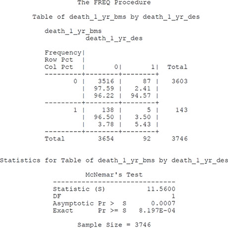
We conducted a sensitivity analysis to determine the sensitivity of the observed effect of treatment on mortality to unmeasured confounders. There were 225 discordant pairs. Of these, 138 were pairs in which the BMS patient died and the DES patient did not. For a given value of Γ, Rosenbaum (1995) defines the following two proportions: p+ = Γ /(1 + Γ) and p- = 1/(1 + Γ). Then, the bounds for the significance of the treatment effect if the unmeasured confounder were taken into account are as follows:
where T is McNemar’s statistic and m denotes the observed data. The exact boundaries of the significance levels can be determined for different values of Γ using the following SAS code in Program 3.5.
Program 3.5 SAS Code for Examining the Sensitivity of the Propensity Score Matched Analysis to an Unmeasured Confounding Variable
data gamma;
do gamma_init = 0 to 5;
gamma = 1 + gamma_init/20;
p_plus = gamma/(1 + gamma);
p_neg = 1/(1 + gamma);
p_upper = 2*(1 - probbnml(p_plus,225,137) );
p_lower = 2*(1 - probbnml(p_neg,225,137) );
output;
end;
run;
proc print data=gamma noobs;
var gamma p_plus p_neg p_lower p_upper;
title "Sensitivity analysis for McNemar's test";
run;
Output from Program 3.5
Sensitivity analysis for McNemar's test
| gamma | p_plus | p_neg | p_lower | p_upper |
| 1.00 | 0.50000 | 0.50000 | .000819738 | 0.000820 |
| 1.05 | 0.51220 | 0.48780 | .000206443 | 0.002869 |
| 1.10 | 0.52381 | 0.47619 | .000049244 | 0.008434 |
| 1.15 | 0.53488 | 0.46512 | .000011232 | 0.021289 |
| 1.20 | 0.54545 | 0.45455 | .000002469 | 0.047026 |
| 1.25 | 0.55556 | 0.44444 | .000000527 | 0.092418 |
If there was an unmeasured binary variable that increased the odds of exposure by no more than 20%, the statistical significance of the observed treatment effect would be at most 0.047. However, if there was an unmeasured binary variable that increased the odds of exposure by 25%, and if this variable was almost perfectly associated with mortality, then the significance level of the treatment effect could be as large as 0.092.
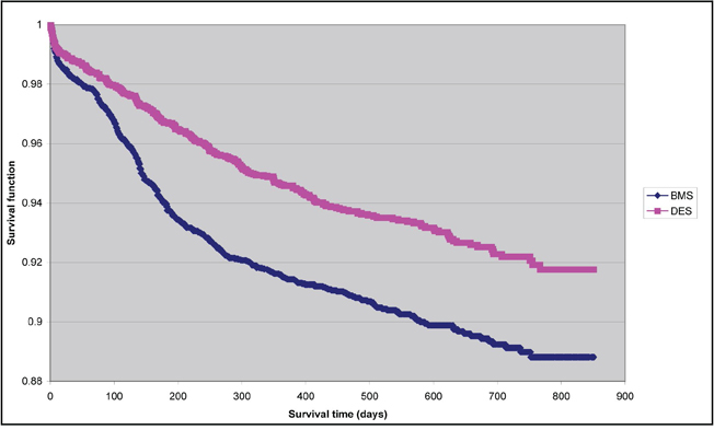
The efficacy outcome we considered was a time-to-event outcome: time to total vessel revascularization. Figure 3.2 depicts the Kaplan-Meier survival curves in each of the two treatment arms of the study. Survival free of total vessel revascularization was better in the DES group than it was in the BMS group. The difference between the survival curves was significant, according to the test proposed by Klein and Moeschberger (1997) (P < 0.0001). The SAS code for assessing the difference between the survival curves is shown in Program 3.6.
Figure 3.2 Kaplan-Meier Survival Curves in PS-Matched Sample: Time to Target Vessel Revascularization
Program 3.6 SAS Code for Comparing the Kaplan-Meier Survival Curves between DES and BMS Patients in the Propensity Score Matched Sample
data long;
set long;
if des = 1 then stent = "DES";
else stent = "BMS";
run;
proc lifetest data=long outsurv=kmdata_tvra notable;
time tvra_time*tvra(0);
strata stent;
/* ‘tvra_time’ denotes time to total vessel revascularization */
/* ‘tvra’ is the censoring indicator: 1 indicates that the event
occurred, while */
/* 0 indicates that the subject has been censored. */
/* ‘stent’ denotes the exposure group: DES vs. BMS. */
title 'Kaplan-Meier survival curves for DES and BMS patients';
run;
data km_compare;
set wide_combo;
if (tvra_time_des < tvra_time_bms) and (tvra_des = 0) then delete;
if (tvra_time_bms < tvra_time_des) and (tvra_bms = 0) then delete;
/* Delete pairs in which the shorter of the two observation times */
/* is for a subject who is censored. */
if (tvra_time_des < tvra_time_bms) and (tvra_des = 1) then D1 = 1;
else D1 = 0;
if (tvra_time_bms < tvra_time_des) and (tvra_bms = 1) then D2 = 1;
else D2 = 0;
run;
proc means sum data=km_compare noprint;
var D1 D2;
output out=km_stat (keep = D1 D2) sum = D1 D2;
run;
data km_stat;
set km_stat;
z = (D1 - D2)/sqrt(D1 + D2);
/* Test statistic for comparing K-M curves from matched sample */
p_value = 2*(1 - probnorm(abs(z)));
run;
proc print data=km_stat;
var D1 D2 z p_value;
title 'Comparing K-M survival curve from matched sample';
run;
Output from Program 3.6
Comparing K-M survival curve from matched sample
| Obs | D1 | D2 | z | p_value |
| 1 | 222 | 336 | -4.82600 | .000001393 |
A Cox proportional hazards model was fit to the matched sample. The model contained exposure status as the sole predictor variable, stratified on the matched pairs. The hazard ratio for DES compared to BMS was 0.661 (95% CI = [0.558, 0.783]) (P < 0.0001). When a univariate Cox proportional hazards model was fit and a robust variance estimate was obtained, the associated hazards ratio was 0.683 (95% CI = [0.582, 0.800]) (P < 0.0001). The SAS code for each of these survival regression models is provided in Program 3.7.
Program 3.7 SAS Code for Fitting Cox Proportional Hazards Models in the Propensity Score Matched Sample
/* Cox proportional hazards model stratifying on matched pairs */
proc phreg data=long nosummary;
model tvra_time*tvra(0) = des/ties=exact rl;
strata pair_id;
title 'Cox proportional hazards model stratifying on matched sets';
run;
/* Cox proportional hazards model with robust standard errors to */
/* account for clustering in matched pairs. */
proc phreg data=long covs(aggregate);
model tvra_time*tvra(0) = des/ties=exact rl;
id pair_id;
title 'Cox proportional hazards model with robust standard errors';
run;
Output from Program 3.7
Cox proportional hazards model stratifying on matched sets
The PHREG Procedure
Model Information
| Data Set | WORK.LONG |
| Dependent Variable | tvra time |
| Censoring Variable | tvra |
| Censoring Value(s) | 0 |
| Ties Handling | EXACT |
| Number of Observations Read | 7492 |
| Number of Observations Used | 7492 |
Convergence Status
Convergence criterion (GCONV=1E-8) satisfied.
Model Fit Statistics
| Criterion | Without Covariates | With Covariates |
| −2 LOG L | 773.552 | 750.097 |
| AIC | 773.552 | 752.097 |
| SBC | 773.552 | 756.532 |
Testing Global Null Hypothesis: BETA=0
| Test | Chi-Square | DF | Pr > ChiSq |
| Likelihood Ratio | 23.4551 | 1 | <.0001 |
| Score | 23.2903 | 1 | <.0001 |
| Wald | 22.9594 | 1 | <.0001 |
Analysis of Maximum Likelihood Estimates
| Variable | DF | Parameter Estimate | Standard Error | Chi-Square | Pr > ChiSq |
| des | 1 | -0.41443 | 0.08649 | 22.9594 | <.0001 |
Analysis of Maximum Likelihood Estimates
| Variable | Hazard Ratio | 95% Hazard Confidence | Ratio Limits |
| des | 0.661 | 0.558 | 0.783 |
Cox proportional hazards model with robust standard errors
The PHREG Procedure
Model Information
| Data Set | WORK.LONG |
| Dependent Variable | tvra time |
| Censoring Variable | tvra |
| Censoring Value(s) | 0 |
| Ties Handling | EXACT |
| Number of Observations Read | 7492 |
| Number of Observations Used | 7492 |
Summary of the Number of Event and Censored Values
| Total | Event | Censored | Percent Censored |
| 7492 | 623 | 6869 | 91.68 |
Convergence Status
Convergence criterion (GCONV=1E-8) satisfied.
Model Fit Statistics
| Criterion | Without Covariates | With Covariates |
| −2 LOG L | 10307.321 | 10284.920 |
| AIC | 10307.321 | 10286.920 |
| SBC | 10307.321 | 10291.920 |
Testing Global Null Hypothesis: BETA=0
| Test | Chi-Square | DF | Pr > ChiSq |
| Likelihood Ratio | 22.4071 | 1 | <.0001 |
| Score (Model-Based) | 22.3257 | 1 | <.0001 |
| Score (Sandwich) | 22.1856 | 1 | <.0001 |
| Wald (Model-Based) | 22.0567 | 1 | <.0001 |
| Wald (Sandwich) | 22.1776 | 1 | <.0001 |
Analysis of Maximum Likelihood Estimates
| Variable | DF | Parameter Estimate | Standard Error | Chi-Square | Pr > ChiSq |
| des | 1 | -0.41443 | 0.08649 | 22.9594 | <.0001 |
Cox proportional hazards model with robust standard errors
The PHREG Procedure
Analysis of Maximum Likelihood Estimates
| Variable | Hazard Ratio | 95% Hazard Confidence | Ratio Limits |
| des | 0.683 | 0.582 | 0.800 |
Three recent systematic reviews found that propensity score matching was poorly implemented in the medical literature overall between 1996 and 2003 (Austin, 2008b) and, in a more recent era, in the cardiovascular surgery literature between 2004 and 2006 (Austin, 2007a) and in the general cardiology literature between 2004 and 2006 (Austin, 2008d). Indeed, in the first review of 47 articles, it was found that only two studies conducted all aspects of propensity score matching correctly, while in the second review it was found that none of the 60 articles examined conducted all of the statistical analyses correctly. Similar findings were observed in the third review. Common errors included employing inappropriate methods for assessing the balance of measured baseline covariates between treated and untreated subjects in the propensity score matched sample and failing to account for the matched nature of the sample when estimating the variance of the treatment effect. Furthermore, many studies did not provide sufficient detail on how the propensity score matched pairs were formed, thereby limiting the ability of other researchers to replicate the study methods.
In this chapter, we have discussed and illustrated the use of propensity score matching for estimating causal treatment effects. In particular, there are four important components to properly conducting an analysis using propensity score matching. First, specify the propensity score model. Second, create matched sets of treated and untreated subjects by matching on the propensity score. Fully report how the propensity score matched sample was formed. This allows other researchers to replicate your study methods and thereby confirm the findings of your study. Third, assess whether matching on the propensity score has resulted in a matched sample in which the distribution of measured baseline covariates are similar between treated and untreated subjects. Investigators should employ sample-specific methods for assessing the similarity of the distribution of measured covariates between treated and untreated subjects. The first three steps may need to be repeated iteratively until an acceptable balance between treated and untreated subjects has been achieved. Finally, statistical methods that account for the matched nature of the propensity score matched sample should be employed for estimating the treatment effect and its statistical significance.
The Institute for Clinical Evaluative Sciences (ICES) and the PATH Research Institute are supported in part by a grant from the Ontario Ministry of Health and Long-Term Care (MOHLTC). The opinions, results, and conclusions are those of the authors, and no endorsement by the Ministry of Health and Long-Term Care or by the Institute for Clinical Evaluative Sciences is intended or should be inferred. Dr. Austin is supported in part by a Career Investigator award from the Heart and Stroke Foundation of Ontario. Dr. Ko is supported in part by a Clinician Scientist award from the Heart and Stroke Foundation of Ontario. Dr. Tu is supported by a Tier 1 Canada Research Chair in Health Services Research and a Career Investigator award from the Heart and Stroke Foundation of Ontario. The authors wish to acknowledge the Ontario Health Technology Advisory Committee (OHTAC) for funding support for the comparative stent study in Ontario. The authors acknowledge that the clinical registry data used in this chapter are from the Cardiac Care Network of Ontario and its member hospitals. The Cardiac Care Network of Ontario serves as an advisory body to the MOHLTC and is dedicated to improving the quality, efficiency, access, and equity in the delivery of the continuum of adult cardiac services in Ontario, Canada. The Cardiac Care Network of Ontario is funded by the MOHLTC.
Agresti, A., and Y. Min. 2004. “Effects and non-effects of paired identical observations in comparing proportions with binary matched-pairs data.” Statistics in Medicine. 23: 65–75.
Austin, P. C. 2007a. Propensity-score matching in the cardiovascular surgery literature from 2004 to 2006: a systematic review and suggestions for improvement.” Journal of Thoracic and Cardiovascular Surgery 134: 1128–1135.
Austin, P. C. 2007b. “The performance of different propensity score methods for estimating marginal odds ratios.” Statistics in Medicine 26: 3078–3094.
Austin, P. C. 2008a. “Assessing balance in baseline covariates when using many-to-one propensity-score matching.” Pharmacoepidemiology and Drug Safety 17: 1218–1225.
Austin, P. C. 2008b. “A critical appraisal of propensity-score matching in the medical literature between 1996 and 2003.” Statistics in Medicine 27 (12): 2037–2049.
Austin, P. C. 2008c. “The performance of different propensity-score methods for estimating relative risks. Journal of Clinical Epidemiology 61 (6): 537–545.
Austin, P. C. 2008d. “Primer on statistical interpretation or methods report card on propensity-score matching in the cardiology literature from 2004 to 2006: A systematic review.” Circulation: Cardiovascular Quality and Outcomes 1(1): 62–67.
Austin, P. C. 2009a. “Some methods of propensity-score matching had superior performance to others: results of an empirical investigation and Monte Carlo simulations.” Biometrical Journal 51: 171–184.
Austin, P.C. 2009b. “Balance diagnostics for comparing the distribution of baseline covariates between treatment groups in propensity-score matched samples.” Statistics in Medicine 28: 3083-3107.
Austin, P.C. 2009c. “Type 1 Error Rates, Coverage of Confidence Intervals, and Variance Estimation in Propensity-score Matched Analyses.” The International Journal of Biostatistics 5: Article 13. DOI: 10.2202/1557-4679.1146.
Austin, P.C. 2009d. “The relative ability of different propensity-score methods to balance measured covariates between treated and untreated subjects in observational studies.” Medical Decision Making 29:661-677.
Austin, P. C., and M. M. Mamdani. 2006. “A comparison of propensity score methods: a case-study estimating the effectiveness of post-AMI statin use.” Statistics in Medicine. 25: 2084–2106.
Austin, P. C., M. M. Mamdani, D. N. Juurlink, and J. E. Hux. 2006. “Testing multiple statistical hypotheses resulted in spurious associations: a study of astrological signs and health.” Journal of Clinical Epidemiology 59: 964–969.
Austin, P. C., M. M. Mamdani, T. A. Stukel, G. M. Anderson, and J. V. Tu. 2005. “The use of the propensity score for estimating treatment effects: administrative versus clinical data.” Statistics in Medicine. 24: 1563–1578.
Austin, P. C., P. Grootendorst, and G. M. Anderson. 2007a. “A comparison of the ability of eifferent propensity score models to balance measured variables between treated and untreated subjects: a Monte Carlo study.” Statistics in Medicine 26: 734–753.
Austin, P. C., P. Grootendorst, S. L. T. Normand, and G. M. Anderson. 2007b. “Conditioning on the propensity score can result in biased estimation of common measures of treatment effect: a Monte Carlo study.” Statistics in Medicine 26: 754–768.
Cochran, W. G., and D. B. Rubin. 1973. “Controlling bias in observational studies: a review.” Sankhya Series A 35: 417–446.
Conover, W. J. 1998. Practical Nonparametric Statistics. 3d ed. New York: John Wiley & Sons, Inc.
Cook, R. J., and D. L. Sackett. 1995. “The number needed to treat: a clinically useful measure of treatment effect.” British Medical Journal 310: 452–454.
Cummings, P., B. McKnight, and S. Greenland. 2003. “Matched cohort methods for injury research.” Epidemiologic Reviews 25: 43–50.
Diggle, P. J., K. Y. Liang, S. L. Zeger, and P. Heagerty. 1994. Analysis of Longitudinal Data. Oxford: Oxford University Press.
Flury, B. K., and H. Riedwyl. 1986. “Standard distance in univariate and multivariate analysis.” The American Statistician 40: 249–251.
Freemantle, N. 2001. “Interpreting the results of secondary end points and subgroup analyses in clinical trials: should we lock the crazy aunt in the attic?” British Medical Journal 322: 989–991.
Hansen, B.B. 2004. “Full matching in an observational study of coaching for the SAT.” Journal of the American Statistical Association 99: 609–618.
Hansen, B. B. 2008. “The essential role of balance tests in propensity-matched observational studies: comments on ‘A critical appraisal of propensity-score matching in the medical literature between 1996 and 003’.” Statistics in Medicine 27: 2050–2054.
Hill, J., and J. P. Reiter. 2006. “Interval estimation for treatment effects using propensity score matching.” Statistics in Medicine 25: 2230–2256.
Ho, D. E., K. Imai, G. King, and E. A. Stuart. 2007. “Matching as nonparametric preprocessing for reducing model dependence in parametric causal inference.” Political Analysis 15: 199–236.
Imai, K., G. King, and E. A. Stuart. 2008. “Misunderstandings between experimentalists and observationalists about causal inference.” Journal of the Royal Statistical Society, Series A (Statistics in Society) 171: 481–502.
Jaeschke, R., G. Guyatt, H. Shannon, S. Walter, D. Cook, and N. Heddle. 1995. “Basic statistics for clinicians: 3. Assessing the effects of treatment: measures of association.” Canadian Medical Association Journal 152 (3): 351–357.
Klein, J. P., and M. L. Moeschberger. 1997. Survival Analysis: Techniques for Censored and Truncated Data. New York: Springer-Verlag.
Lin, D. 1989. “Goodness-of-fit tests and robust statistical inference for the Cox proportional hazards model.” Journal of the American Statistical Association 84: 1074–1078.
Newcombe, R. G. 2006. “A deficiency of the odds ratio as a measure of effect size.”
Statistics in Medicine 25: 4235–40.
Normand, S. T., M. B. Landrum, E. Guadagnoli, et al. 2001. “Validating recommendations for coronary angiography following acute myocardial infarction in the elderly: a matched analysis using propensity scores.” Journal of Clinical Epidemiology 54(4): 387–98.
Rosenbaum, P. R. 1987. “Model-based direct adjustment.” The Journal of the American Statistical Association 82: 387–394.
Rosenbaum, P. R. 1995. Observational Studies. New York: Springer-Verlag.
Rosenbaum, P. R., and D. B. Rubin. 1983a. “The central role of the propensity score in observational studies for causal effects.” Biometrika 70: 41–55.
Rosenbaum, P. R., and D. B. Rubin. 1983b. “Assessing sensitivity to an unobserved binary covariate in an observational study with binary outcome.” Journal of the Royal Statistical Society, B (StatisticalMethodology) 45: 212–218.
Rosenbaum, P. R., and D. B. Rubin. 1984. “Reducing bias in observational studies using subclassification on the propensity score.” Journal of the American Statistical Association 79: 516–524.
Rosenbaum, P. R., and D. B. Rubin. 1985. “Constructing a control group using multivariate matched sampling methods that incorporate the propensity score.” The American Statistician 39: 33–38.
Rothman, K. J. 1977. “Epidemiologic methods in clinical trials.” Cancer 39 (S4): 1771–1775.
Rothman, K. J., and S. Greenland. 1998. Modern Epidemiology. Philadelphia, PA: Lippincott Williams & Wilkins.
Rothwell, P. M. 2005. “Treating individuals 2: Subgroup analysis in randomised controlled trials: importance, indications, and interpretation.” The Lancet 365: 176–186.
Rubin, D. B. 2004. “On principles for modeling propensity scores in medical research.” Pharmacoepidemiology and Drug Safety 13(12): 855–857.
Schechtman, E. 2002. “Odds ratio, relative risk, absolute risk reduction, and the number needed to treat––which of these should we use?” Value in Health 5(5): 431–436.
Senn, S. 1994. “Testing for baseline balance in clinical trials.” Statistics in Medicine 13: 1715–1726.
Senn, S. J. 1989. “Covariate imbalance and random allocation in clinical trials.” Statistics in Medicine 8: 467–475.
Sinclair, J. C., M. B. Bracken. 1994. “Clinically useful measures of effect in binary analyses of randomized trials.” Journal of Clinical Epidemiology 47(8): 881–889.
Therneau, T. M., and P. M. Grambsch. 2001. Modeling Survival Data: Extending the Cox Model. New York: Springer-Verlag.
Tu, J. V., J. Bowen, M. Chiu, D. T. Ko, P. C. Austin, Y. He, R. Hopkins, J. Tarride, G. Blackhouse, C. Lazzam, E. A. Cohen, and R. Goeree. 2007. “Effectiveness and safety of drug-eluting stents in Ontario.” The New England Journal of Medicine 357(14): 1393–1402.
Weitzen, S., K. L. Lapane, A. Y. Toledano, A. L. Hume, and V. Mor. 2005. “Weakness of goodness-of-fit tests for evaluating propensity score models: the case of the omitted confounder.” Pharmacoepidemiolgy and Drug Safety 14(4): 227–238.
1 These SAS macros were written locally and are maintained by Mayo Clinic staff. They contain the SAS source code, a brief description of the macro's function, and an example of the macro call. Copyright 2005 Mayo Foundations for Medical Education and Research. This software is free software; you can redistribute it and/or modify it under the terms of the GNU General Public License as published by the Free Software Foundation; either version 2 of the License, or (at your option) any later version. These macros are distributed in the hope that they will be useful, but WITHOUT ANY WARRANTY; without even the implied warranty of MERCHANTABILITY or FITNESS FOR A PARTICULAR PURPOSE. See the GNU General Public License for more details. If you use functions from the Mayo Clinic, please acknowledge the original contributor of the material.