Chapter 15

Incremental Net Benefit

Andrew R. Willan

Abstract

15.1 Introduction

15.2 Cost-Effectiveness Analysis

15.3 Parameter Estimation

15.4 Example

15.5 Observational Studies

15.6 Discussion

Acknowledgments

References

 

Abstract

Since the early 1990s, motivated by the availability of patient-level cost data in clinical studies for comparing patient groups, researchers have made rapid developments in statistical methods for cost-effectiveness data. Initial efforts concentrated on inference about the incremental cost-effectiveness ratio, but due to difficulties associated with ratio statistics, interest has settled more recently on incremental net benefit. Regardless of the approach, five parameters need to be estimated: the between-treatment arm differences in mean effectiveness and mean cost and the corresponding variances and covariance. With these parameter estimates, the analyst can estimate the incremental cost-effectiveness ratio and calculate the corresponding confidence limits. Due to concerns regarding ratio statistics, the analyst may choose to focus on the incremental net benefit. Taking a traditional Frequentist’s approach, the incremental net benefit can be estimated, with the uncertainty being characterized by the corresponding confidence limits. Alternatively, taking a Bayesian approach, the cost-effectiveness acceptability curve can be used to display the magnitude of the between-group contrast and to characterize its uncertainty. A review of these methods is given. The particular statistical procedure used for estimating the five parameters depends on:

• whether censoring is present

• whether covariates are adjusted for

• whether random effects, such as country, are adjusted for

• what the assumptions are regarding the distribution for cost

A brief review of the statistical procedures, particular to each combination of these conditions, is given, where they exist. An example of a randomized clinical trial is provided.

 

15.1 Introduction

Since the early 1990s, it has become more common for resource utilization data to be collected in clinical studies. The resource data, combined with unit price weights, provide a measure of total cost at the patient level, in addition to measures of effectiveness. Having measures of effectiveness and cost at the patient level permits the use of conventional methods of statistical inference for quantifying the uncertainty due to sampling and measurement error. Numerous articles have been published on the statistical analysis of cost-effectiveness data. Initial efforts concentrated on providing confidence intervals for the incremental cost-effectiveness ratio (ICER), which is the between-treatment difference in mean cost divided by the between-treatment difference in mean effectiveness. However, due to concerns regarding ratio statistics, the concept of incremental net benefit (INB) has been adopted as an alternative. The INB is the increase in effectiveness, expressed in monetary terms, minus the increase in cost. The purpose of this chapter is to provide a structured review of commonly proposed methods for a statistical cost-effectiveness analysis (CEA), with emphasis on the INB. The context used throughout the paper is that of a two-arm randomized clinical trial where patients are randomized to treatment (arm T) or standard (arm S). However, the methods apply to the comparison of any two groups, subject to the concerns one might have regarding bias due to the lack of random group allocation (see Section 15.5 for further discussion).

In a parametric approach, the essential task of a CEA is to jointly model effectiveness and cost to estimate five parameters. Two of the parameters are the between-treatment arm differences in mean effectiveness, denoted by Δ_e, and the between-treatment arm differences, and the between-treatment arm differences in mean cost, denoted by Δ_c. The other three parameters are the variance of the estimator of Δ_e, denoted by $V({\hat{\mathrm{\Delta }}}_e)$; the variance of the estimator of Δ_c, denoted by $V({\hat{\mathrm{\Delta }}}_c)$; and the covariance of the estimators of Δ_e and Δ_c, denoted by $C({\hat{\mathrm{\Delta }}}_e,{\hat{\mathrm{\Delta }}}_c)$, where $\hat{\theta }$ indicates the estimator of θ. Effectiveness and cost must be modeled jointly to enable the estimation of the covariance. The particular statistical procedure used for estimating the five parameters depends on the following:

• whether censoring is present

• whether covariates are adjusted for

• whether random effects such as country are adjusted for

• what the assumptions are regarding the distribution for cost

With the estimators of these five parameters, a CEA, based on either the incremental cost-effectiveness ratio or the incremental net benefit, can be performed. Throughout the rest of this chapter, it is assumed that the estimators of Δ_e and Δ_c are normally distributed. This assumption relies on the central limit theorem, which holds that the sum of a large number of independent random variables will tend to follow a normal distribution.

In Section 15.2, the methods used to display a CEA, based on the five parameter estimates, are illustrated. The statistical procedures used to estimate the parameters, which depend on the issues discussed earlier, are reviewed in Section 15.3. An example using data from a randomized clinical trial is given in Section 15.4. Section 15.5 discusses the issues specific to observational studies. A summary of the chapter follows in Section 15.6.

 

15.2 Cost-Effectiveness Analysis

A general introduction to the cost-effectiveness analysis associated with the comparison of two groups is given in this section. Typically, though not necessarily, the measure of effectiveness in a CEA is associated with a clinical event experienced by the patient, such as death, relapse, or reaching a pre-specified level of symptom relief. The three measures of effectiveness associated with an event, death for example, are

1. whether the patient survived for the duration of interest

2. the survival time over the duration of interest

3. the quality-adjusted survival time over the duration of interest

Correspondingly, Δ_e is

1. the between-treatment difference in the probability of surviving

2. the between-treatment difference in the mean survival time

3. the between-treatment difference in the mean quality-adjusted survival time

All means are restricted to the duration of interest and the difference is taken as T − S, so that positive differences favor T. The ICER is defined by Δ_c/Δ_e where the difference for Δ_c is taken as T − S. Therefore the ICER is, respectively,

1. the additional cost of saving a life from using T rather than S

2. the additional cost of an extra year of life gained from using T rather than S

3. the additional cost of a quality-adjusted life-year (QALY) from using T rather than S

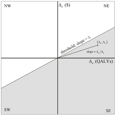
The ICER can be illustrated on the cost-effectiveness plane, as shown in Figure 15.1, as the slope of the line between the origin and the point . (Δ_e, Δ_c)

In Figures 15.1 through 15.5, we have assumed that the measure of effectiveness is quality-adjusted survival time and the unit of effectiveness is quality-adjusted life-years (QALYs). Also shown in Figure 15.1 is a line, referred to as the threshold, through the origin with the slope equal to the threshold willingness-to-pay (WTP) for a unit of effectiveness, denoted as λ. The threshold divides the cost-effectiveness plane into two regions. For points on the plane below and to the right of the threshold (shaded), T is considered cost-effective, but for those above and to the left, it is not. Because λ is positive, points in the SE quadrant, where T is more effective and less costly, are always below the threshold and therefore correspond to comparisons for which T is cost-effective. On the other hand, points in the NW quadrant, where T is less effective and more costly, are always above the threshold and correspond to comparisons for which T is not cost-effective. It is in the NE and SW quadrants that the concept of threshold WTP allows for a tradeoff between effectiveness and cost. In the NE quadrant, the slope of any point below the line is less than λ (that is, for any point below the threshold $\frac{{\mathrm{\Delta }}_c}{{\mathrm{\Delta }}_e}<\lambda$), which implies that ${\mathrm{\Delta }}_c<{\mathrm{\Delta }}_e\lambda$.

Therefore, the increase in value (Δ_e λ) is greater than the increase in cost, making T cost-effective. In the SW quadrant, the slope of any point below the line is greater than λ, and because Δ_e and Δ_c are both negative (that is, treatment is less effective and less costly), we have $\frac{{\mathrm{\Delta }}_c}{{\mathrm{\Delta }}_e}=\frac{\left|{\mathrm{\Delta }}_c\right|}{\left|{\mathrm{\Delta }}_e\right|}>\lambda$, which implies that |Δ_c|>|Δ_e λ. Therefore, the value lost (|Δ_eλ|) is less than the amount saved (|Δ_c|), making T cost-effective. In summary, T is cost-effective if, and only if,

$A:\hspace{1em}\frac{{\mathrm{\Delta }}_c}{{\mathrm{\Delta }}_e}<\lambda \hspace{1em}if\&{\mathrm{\Delta }}_e>0;\hspace{1em}or\hspace{1em}\frac{{\mathrm{\Delta }}_c}{{\mathrm{\Delta }}_e}>\lambda \hspace{1em}if\&{\mathrm{\Delta }}_e<0.$                                 (1)

Equation 1 (Hypothesis A) defines the region below the threshold and can be thought of as the alternative hypothesis for the null hypothesis H, given by:

$H:\hspace{1em}\frac{{\mathrm{\Delta }}_c}{{\mathrm{\Delta }}_e}\ge \lambda \hspace{1em}if\&{\mathrm{\Delta }}_e>0;\hspace{1em}or\hspace{1em}\frac{{\mathrm{\Delta }}_c}{{\mathrm{\Delta }}_e}\le \lambda \hspace{1em}if\&{\mathrm{\Delta }}_e<0.$                                  (2)

Rejecting H in favor of A would provide evidence to adopt T. These equations are somewhat awkward and can be simplified considerably by the introduction of INB.

Figure 15.1 The Cost-Effectiveness Plane

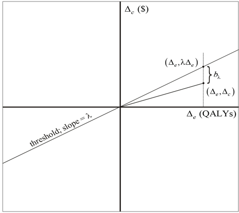
The INB is a function of λ and is defined as $b_{\lambda }\equiv {\mathrm{\Delta }}_e\lambda -{\mathrm{\Delta }}_c.b_{\lambda }$ is the incremental net benefit because it is the difference between the incremental value (Δ_eλ) and the incremental cost (Δ_c). T is cost-effective if, and only if, b_λ > 0, regardless of the sign of Δ_e. To see this, both inequalities involving the ICER in Equation 1 can be rearranged to the inequality ${\mathrm{\Delta }}_e\lambda -{\mathrm{\Delta }}_c>0$. Similarly, both inequalities involving the ICER in Equation 2 can be rearranged to the inequality ${\mathrm{\Delta }}_e\lambda -{\mathrm{\Delta }}_c\le 0$. Therefore, in terms of INB the null and alternative hypotheses become simplified as:

$H:b_{\lambda }\le 0\hspace{1em}versus\hspace{1em}A:b_{\lambda }>0 .$                                 (3)

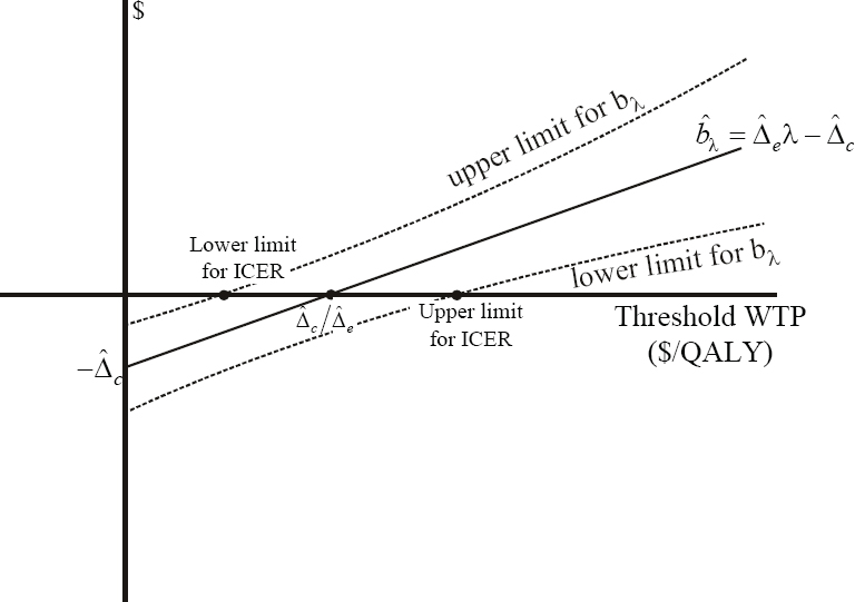
The formulations of hypotheses H and A given in Equations 1, 2, and 3 illustrate the close relationship between the ICER and the INB. On the cost-effectiveness plane, b_λ is the vertical distance from the point (Δ_e, Δ_c) to the threshold, being positive if the point is below the line and negative otherwise. Because it has a slope of, the point on the threshold with abscissa equal to Δ_e is (Δ_e, Δ_eλ) and so the vertical distance between it and (Δ_e, Δ_c) is Δ_eλ - Δ_c (see Figure 15.2).

Figure 15.2 INB on the Cost-Effectiveness Plane

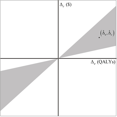
The ICER can be estimated by ${\hat{\mathrm{\Delta }}}_c/{\hat{\mathrm{\Delta }}}_e,$ where ${\hat{\mathrm{\Delta }}}_c$ and ${\hat{\mathrm{\Delta }}}_e$ are the estimators of Δ_c and Δ_e, respectively. The estimator ${\hat{\mathrm{\Delta }}}_c/{\hat{\mathrm{\Delta }}}_e$ is biased, but it is consistent if ${\hat{\mathrm{\Delta }}}_c$ and ${\hat{\mathrm{\Delta }}}_e$ are unbiased, meaning that the bias diminishes as the sample size increases (Chaudary and Stearns, 1996; Cochran, 1997). Statistical inference for the ICER has been restricted to calculating its confidence interval. Applying Fieller’s theorem [1, 3], the confidence limits are given by

$R\left\{\left(1-z_{1-\alpha }^{2}c\pm z_{1-\alpha }\sqrt{a+b-2c-z_{1-\alpha }^2(ab-c^2)}\right)/\left(1-z_{1-\alpha }^{2}a\right)\right\},$         (4)

Where, $R={\hat{\mathrm{\Delta }}}_c/{\hat{\mathrm{\Delta }}}_{e}a=\hat{V}\left({\hat{\mathrm{\Delta }}}_e\right)/{\hat{\mathrm{\Delta }}}_e^{2}b=\hat{V}\left({\hat{\mathrm{\Delta }}}_c\right)/{\hat{\mathrm{\Delta }}}_c^{2}c=\hat{C}\left({\hat{\mathrm{\Delta }}}_e,{\hat{\mathrm{\Delta }}}_c\right)/\left({\hat{\mathrm{\Delta }}}_e{\hat{\mathrm{\Delta }}}_c\right)$ and $z_{1-\alpha }$ is the 100(1−α)th percentile of the standard normal random variable. The set of points on the cost-effectiveness plane, whose slopes are between the limits defined in Equation 4, define a “bow tie” region on the cost-effectiveness plane (see Figure 15.3), but inference is usually restricted to the region of the bow tie that includes the point $({\hat{\mathrm{\Delta }}}_e,{\hat{\mathrm{\Delta }}}_c)$. If $a+b-2c-z_{1-\alpha }^2(ab-c^2)<0$, then Equation 4 has no solution and neither limit is defined, meaning that the data are too close in probability to the origin for an analysis to provide, with high confidence, inference regarding the value of the ICER. The ICER has other weaknesses. It cannot be interpreted without specifying the sign of either Δ_e or Δ_c). Also, the estimator of the ICER has an undefined mean and variance.

Figure 15.3 Bow Tie ICER Confidence Region

These difficulties, plus the fact that the ICER is not properly ordered on the non-tradeoff (SE and NW) quadrants of the cost-effectiveness plane, have led analysts to make inferences regarding cost-effectiveness with respect to INB as an alternative. As stated previously, T is cost-effective if, and only if, b_λ >0, and taking a Bayesian approach, the cost-effectiveness acceptability curve (CEAC) is a plot of the probability that b_λ >0 as a function of λ. Assuming no prior information,the CEAC can be given by $CEAC(\lambda )=\mathrm{\Phi }\left({\hat{b}}_{\lambda }/SE({\hat{b}}_{\lambda })\right)$, where $\Phi (\dot{})$ is the cumulative distribution function for the standard normal ${\hat{b}}_{\lambda }={\hat{\mathrm{\Delta }}}_e\lambda -{\hat{\mathrm{\Delta }}}_c$ random variable and is the estimator of with standard error $SE({\hat{b}}_{\lambda }),$ given by $\sqrt{{\lambda }^2\hat{\mathrm{V}}\left({\hat{\mathrm{\Delta }}}_e\right)+\hat{\mathrm{V}}\left({\hat{\mathrm{\Delta }}}_c\right)-2\lambda \hat{\mathrm{C}}\left({\hat{\mathrm{\Delta }}}_e,{\hat{\mathrm{\Delta }}}_c\right)}$. Estimating the CEAC by $\Phi \left({\hat{b}}_{\lambda }/\mathrm{SE}({\hat{b}}_{\lambda })\right)$assumes that ${\hat{\mathrm{\Delta }}}_e$ and ${\hat{\mathrm{\Delta }}}_c$ are normally distributed. This assumption relies on the central limit theorem. For a more complete discussion of the Bayesian framework in cost-effectiveness, see O’Hagan and Stevens (2001).

The CEAC has the advantage of capturing both the magnitude and uncertainty of the observed cost-effectiveness. It also allows readers to apply the threshold WTP that is most appropriate for them. As illustrated in Figure 15.4, the CEAC passes through 0.5 at λ, equal to the ICER and through α and 1 -α at λ equal to the ICER Fieller limits defined here. Therefore, the CEAC, although based on the INB, provides inference regarding the ICER. For more on CEACs, see Fenwick, O’Brien, and Briggs (2004). More direct inference based on INB is provided by plotting its estimate and confidence limits as a function of λ (see Figure 15.5). Confidence limits for the INB are given by ${\hat{b}}_{\lambda }\pm z_{1-\alpha }\text{SE}({\hat{b}}_{\lambda })$. The close relationship between b_λ and the ICER is illustrated in Figure 15.5. The plot of ${\hat{b}}_{\lambda }$ crosses the horizontal axis at the ICER. If ${\hat{\mathrm{\Delta }}}_e$ is positive, the lower limit for b_λ crosses the horizontal axis at the upper Fieller limit for the ICER and the upper limit for b_λ at the lower Fieller limit for the ICER. On the other hand, if ${\hat{\mathrm{\Delta }}}_e$ is negative, the lower limit for b_λ crosses the horizontal axis at the lower Fieller limit for the ICER and the upper limit for b_λ at the upper Fieller limit for the ICER.

Figure 15.4 The Cost-Effectiveness Acceptability Curve

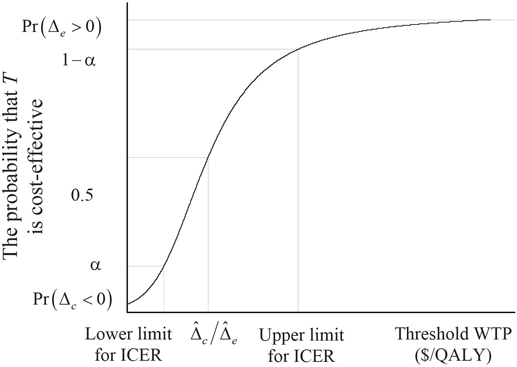
Figure 15.5 Incremental Net Benefit as a Function of WTP (λ)

The CEAC and the plot of b_λ and its confidence limits provide a comprehensive summary of the cost-effectiveness analysis of comparison of two groups. Both graphs can be determined using only the estimators of ${\mathrm{\Delta }}_e,{\mathrm{\Delta }}_c,\text{V}\left({\hat{\mathrm{\Delta }}}_e\right),\text{V}\left({\hat{\mathrm{\Delta }}}_c\right)\text{and C}\left({\hat{\mathrm{\Delta }}}_e,{\hat{\mathrm{\Delta }}}_c\right)$. As discussed previously, how these estimators are determined depends on the nature and sampling of the data. The estimation procedures are reviewed in Section 15.3. The validity of the CEAC and the plots based on INB depend on the assumption that the threshold is a straight line through the origin (that is, λ is invariant to Δ_e). For a discussion of the relaxation of this assumption, see O’Brien and colleagues (2002) and Willan, O’Brien, and Leyva (2001).

 

15.3 Parameter Estimation

Methods used to estimate the parameters required in a CEA are given in this section. A general introduction is given in Section 15.3.1, with more details provided in Section 15.3.2.

 

15.3.1 Introduction to Parameter Estimation

The methods for parameter estimation depend on

• whether censoring is present

• whether covariates are adjusted for

• whether random effects such as center or country are accounted for

• what the assumptions are regarding the distribution for cost

Only simple sample statistics are required for non-censored data with no covariates or random effects and assuming symmetric cost distributions. However, the methods get more complex as fewer of these conditions apply (Willan and Briggs, 2006). The following subsections provide a review of some of the approaches taken. Bootstrap methods, which are often used in a CEA, are not discussed here because their use is intended for situations where no acceptable closed form solution exists [9]. For more on bootstrap methods in cost-effectiveness analysis, see Briggs, Wonderling, and Mooney (1997) and Chapter 4 of Willan and Briggs (2006).

15.3.1.1 Right-Skewing of Cost Data

Because of right-skewing, which is usually in cost data, use of least squares methods such as sample means and variances is often criticized (O’Hagan and Stevens, 2003; Briggs and Gray, 1998; Thompson and Barber, 2000; Nixon and Thompson, 2004; and Briggs et al., 2005). Transformations, such as the logarithm and square root, are sometimes proposed as an alternative. However, such transformations provide estimates on a scale not relevant to decision-makers (Manning and Mullahy, 2001, and Thompson and Barber, 2000). Additionally, a number of investigations into the issue of skewed data, using mostly simulated data, have drawn the conclusion that least squares methods provide valid estimates of mean cost and the between-treatment difference in mean cost. Lumley and colleagues (2002) provide a review of such investigations. Nonetheless, the blind application of sample means and variances to cost data with extreme outliers could lead to misleading conclusions. Faith in the robustness of least squares methodology is no substitute for careful examination of the data using box-plots and histograms. Furthermore, although least squares methods may provide consistent estimators of mean cost, the estimators may be inefficient in the presence of right-skewing.

15.3.1.2 Covariate Adjustment

In randomized clinical trials (RCTs), because covariates tend to be balanced across treatment arms, covariate adjustment may not be necessary, although regression models may be used for improving precision or examining for subgroup effects with the use of interaction terms. However, for observational studies, covariate adjustment is generally considered essential.

15.3.1.3 Censoring

In many clinical trials, some patients are not followed for the entire duration of interest. Some may be lost to follow up, either because they refuse to attend follow-up clinic visits or because they move out of the jurisdiction covered by trial management resources. Also, because of staggered entry and long follow-up times, analysis may be performed before all patients are followed for the entire duration of interest. When censoring is uninformative (that is, the time to death is independent of the time to censoring), life-table methods can be used to provide unbiased estimates of the probability of surviving the duration of interest and the mean survival time. However, for cost and quality-adjusted survival time, the censoring is informative, even if the time to censoring and the time to death are independent, and the use of life-table methods will yield biased estimates (Willan et al., 2002). Consequently, more complex methods must be used to estimate mean quality-adjusted survival time and mean cost. Throughout this chapter, the terms mean survival time, mean quality-adjusted survival time, and mean cost refer to the mean, restricted to the duration of interest. In a cardiology trial, the duration of interest may be 30 days or 12 months; however, in a cancer trial, it could be as long as 5 or 10 years.

15.3.1.4 Random Effects

Many studies are often conducted in more than one country. The advantages are an increase in statistical power, resulting from an increase in sample size, and the perception of greater generalizability. However, the analyses of multinational studies often ignore the possibility of a treatment by country interaction, in which the treatment effects vary between countries. In the presence of an interaction, estimates of treatment effects (that is, between-treatment differences in mean cost and effectiveness) that ignore country effects will have inappropriately small variances and lead to inflated type I errors. Models that treat country as a fixed effect (Wilke et al., 1998; Cook et al., 2003) to account for the interaction have no parameter for the overall treatment effect and provide estimates of the country-specific treatment effects that are based solely on the individual country’s data. A number of recent publications (see Grieve et al., 2005; Willan et al., 2005; Manca et al., 2005; Pinto et al., 2005; and Nixon and Thompson, 2005) address this issue by proposing hierarchal models that treat country as a random effect. These models have the advantage of providing an overall estimate of treatment effect and country-specific estimates that use the data from all countries.

 

15.3.2 Details of Parameter Estimation

Let E_ji and C_ji be the observed measure of effectiveness and cost, respectively, for patient i on treatment arm j, where i = 1, 2, … n_j, j = T, S. E_ji is scaled so that larger values correspond to better health outcomes. For a binary outcome, E_ji is 1 for a success and 0 for a failure. As discussed in Section 15.1.4, it is generally recognized that cost data are skewed to the right. In Sections 15.3.2.1 to 15.3.2.4, methods that ignore the issue of skewed cost data are reviewed, and in Section 15.3.2.5, a review is given for methods that accommodate skewed cost data.

15.3.2.1 No Censoring, No Random Effects, No Covariates

If there is no censoring, no random effects, and no covariates, the parameter estimators are simple functions of sample statistics, such as mean, variances, and proportions. The estimated difference in mean effectiveness and cost are given by

${\hat{\mathrm{\Delta }}}_e={\overline{E}}_T-{\overline{E}}_S=\frac{\sum _{i=1}^{n_T}{E}_{Ti}}{n_T}-\frac{\sum _{i=1}^{n_S}{E}_{Si}}{n_S}$ and ${\hat{\mathrm{\Delta }}}_c={\overline{C}}_T-{\overline{C}}_S=\frac{\sum _{i=1}^{n_T}{C}_{Ti}}{n_T}-\frac{\sum _{i=1}^{n_S}{C}_{Si}}{n_S}$.

The estimated variance of ${\hat{\mathrm{\Delta }}}_c$ is given by

$\hat{\mathrm{V}}\left({\hat{\mathrm{\Delta }}}_c\right)=\frac{\sum _{i=1}^{n_T}{\left(C_{Ti}-{\overline{C}}_T\right)}^2}{n_T(n_T-1)}+\frac{\sum _{i=1}^{n_S}{\left(C_{Si}-{\overline{C}}_S\right)}^2}{n_S(n_S-1)}$ or

$\hat{\mathrm{V}}\left({\hat{\mathrm{\Delta }}}_c\right)=\left(\frac{n_T+n_S}{n_T{n}_S}\right)\frac{\sum _{i=1}^{n_T}{\left(C_{Ti}-{\overline{C}}_T\right)}^2+\sum _{i=1}^{n_S}{\left(C_{Si}-{\overline{C}}_S\right)}^2}{(n_T+n_S-2)}$

for homogeneous variance.

If the measure of effectiveness is continuous, then the estimated variance of ${\hat{\mathrm{\Delta }}}_e$ is given by

$\hat{\mathrm{V}}\left({\hat{\mathrm{\Delta }}}_e\right)=\frac{\sum _{i=1}^{n_T}{\left(E_{Ti}-{\overline{E}}_T\right)}^2}{n_T(n_T-1)}+\frac{\sum _{i=1}^{n_S}{\left(E_{Si}-{\overline{E}}_S\right)}^2}{n_S(n_S-1)}$ or

$\widehat{\text{V}}({\widehat{\Delta }}_c)=\left(\frac{n_T+n_S}{n_T{n}_S}\right)\frac{{\displaystyle \sum _{i=1}^{n_T}{(E_{Ti}-{\overline{E}}_T)}^2}+{\displaystyle \sum _{i=1}^{n_S}{(E_{Si}-{\overline{E}}_S)}^2}}{\left(n_T+n_S-2\right)}$

for homogeneous variance.

The estimated covariance between ${\hat{\mathrm{\Delta }}}_e$ and ${\hat{\mathrm{\Delta }}}_c$ is given by

$\hat{C}\left({\hat{\mathrm{\Delta }}}_e,{\hat{\mathrm{\Delta }}}_c\right)=\frac{\sum _{i=1}^{n_T}\left(E_{Ti}-{\overline{E}}_T\right)\left(C_{Ti}-{\overline{C}}_T\right)}{n_T(n_T-1)}+\frac{\sum _{i=1}^{n_S}\left(E_{Si}-{\overline{E}}_S\right)\left(C_{Si}-{\overline{C}}_S\right)}{n_S(n_S-1)}$ or

$\hat{C}\left({\hat{\mathrm{\Delta }}}_e,{\hat{\mathrm{\Delta }}}_c\right)=\left(\frac{n_T+n_S}{n_T{n}_S}\right)\frac{\sum _{i=1}^{n_T}\left(E_{Ti}-{\overline{E}}_T\right)\left(C_{Ti}-{\overline{C}}_T\right)+\sum _{i=1}^{n_S}\left(E_{Si}-{\overline{E}}_S\right)\left(C_{Si}-{\overline{C}}_S\right)}{(n_T+n_S-2)}$

for homogeneous covariance.

If the measure of effectiveness is binary, then the estimated variance of ${\hat{\mathrm{\Delta }}}_e$ is given by

$\hat{V}\left({\hat{\mathrm{\Delta }}}_e\right)=\frac{{\overline{E}}_T\left(1-{\overline{E}}_T\right)}{n_T}+\frac{{\overline{E}}_S\left(1-{\overline{E}}_S\right)}{n_S}$,

and the estimated covariance between ${\hat{\mathrm{\Delta }}}_e$ and ${\hat{\mathrm{\Delta }}}_c$ is given by

$\hat{C}\left({\hat{\mathrm{\Delta }}}_e,{\hat{\mathrm{\Delta }}}_c\right)=\frac{\left(\sum _{i=1}^{n_T}{E}_{Ti}{C}_{Ti}/n_T\right)-{\overline{E}}_T{\overline{C}}_T}{n_T}+\frac{\left(\sum _{i=1}^{n_S}{E}_{Si}{C}_{Si}/n_S\right)-{\overline{E}}_S{\overline{C}}_S}{n_S}$

15.3.2.2 No Censoring, No Random Effects, with Covariates

To adjust for covariates when there is no censoring or random effects, Willan, Briggs, and Hoch (2004) propose using seemingly unrelated regression equations. Let there be p_e covariates for effectiveness and p_c covariates for costs. The regression model is given by

E(y) = Xβ,

where $y=\left(\begin{array}{c}e\\ c\end{array}\right)$ and e and c are the vectors of length n_T + n_S of the observed effectiveness and costs, respectively. The matrix $X=\left(\begin{array}{cc}Z& \underset{˜}{0}\\ \underset{˜}{0}& W\end{array}\right)$, where Z is of dimension n_T + n_S by p_e + 2 and contains the covariate values for effectiveness. The first column of Z is a dummy indicator for treatment group (1 for T and 0 for S) and the second column contains all ones to provide an intercept. Similarly, W is of dimension n_T + n_S by p_c + 2 and contains the covariate values for costs. The symbol $\underset{˜}{0}$ represents a matrix of zeroes with the appropriate dimensions. The vector $\beta =\left(\begin{array}{c}\mathrm{\omega }\\ \theta \end{array}\right)$ is the vector of parameters, where the first components of w and θ are Δ_e and Δ_c, respectively. If the covariates for effectiveness and cost are the same, then the ordinary least squares solution provides the best linear unbiased estimators. If one set of covariates is a subset of the other, then the ordinary least squares solution provides the best linear unbiased estimators for the smaller set. In all other situations, efficiency gains are possible from the generalized least squares solution. For estimation details, see Willan, Briggs, and Hoch (2004) and Chapter 6 of Willan and Briggs (2006).

The regression methods given here are most appropriate for continuous measures of effectiveness. One approach for covariate adjustment, when the measure of effectiveness is binary, is to combine the methods proposed by Thompson, Warn, and Turner (2004) for binary regression, which allow for the estimation of risk differences (rather than odds ratios) with those of Nixon and Thompson (2005) for jointly modeling effectiveness and cost. The approach requires the use of Markov chain Monte Carlo simulation. A more accessible, albeit slightly ad hoc, method for binary measures of effectiveness is to use the SAS GENMOD procedure (see Section 15.4).

15.3.2.3 No Censoring, Random Effects, and Covariates

To account for random country effects in a multinational RCT, two general approaches are proposed. The first approach, proposed by Pinto, Willan, and O’Brien (2005) and Willan and colleagues (2005), has two stages. In the first stage, each country is treated as a separate trial and the appropriate methods are used to estimate the five parameters of interest. The appropriate methods may include those that account for censoring or covariates. The country-specific estimates are then combined for overall trial estimates using empirical Bayes procedures in what is, essentially, a bivariate (effectiveness and cost) meta-analysis. The second approach(Grieve et al., 2005; Manca et al., 2005; and Nixon and Thompson, 2005) models effectiveness and cost at the patient level, using a hierarchal model to account for the two sources of error (patient and country).

15.3.2.4 Censoring

If the parameter of interest for effectiveness is the probability of survival or mean survival, then life-table methods using the Kaplan-Meier survival curves can be used to estimate Δ_e (Willan et al., 2003, 2002). For quality-adjusted survival and costs, the censoring is informative even if the time to censoring and the time to death are independent, and the use of life-table methods will yield biased estimates. There are primarily two methods for handling this issue. The first, known as the Lin or direct method, is given in Lin and colleagues (1997) and Willan and Lin (2001). The other, based on inverse probability weighting, is given in Bang and Tsiatis (2000), Lin (2000), Zhao and Tian (2001), and Willan and colleagues (2002). Details for both methods are given in Willan and Briggs (2006), Chapter 3.

For parameter estimation in the presence of covariates, see Lin (2000) and Willan, Lin, and Manca (2005). To account for random country effects in a multinational trial with censored data, the analysis could be stratified by country, yielding estimates of Δ_e and Δ_c and the corresponding variances and covariances for each country. These estimates can then be combined for overall trial estimates using empirical Bayes procedures (Willan et al., 2005; Pinto et al., 2005) as discussed in Section 15.3.2.3.

 

15.3.3 Accounting for Skewness in Cost Data

Jointly modeling cost and effectiveness with asymmetrical distributions for cost can be facilitated using Markov chain Monte Carlo methods, a complete discussion of which is given in Nixon and Thompson (2005). Often a gamma distribution is used to model cost. The gamma distribution appears to be sufficiently flexible for fitting cost data in most situations. The models can handle adjustment for covariates, interaction terms for subgroup analysis, and random effects for country. Again, a more accessible method is facilitated by using PROC GENMOD, as illustrated in Section 15.4.

 

15.4 Example

A detailed example is given in this section. The measure of effectiveness is binary and the cost data are somewhat skewed. Further, there is a binary covariate, which, for cost, has a statistically significant interaction with treatment group.

 

15.4.1 The CD Trial

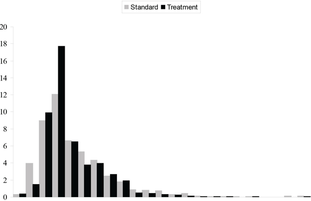
At the request of the principal investigators, the data for this example have been disguised to eliminate any conflict with previous publications. This RCT is referred to as the CD Trial. In the CD Trial, 1,356 patients were recruited and randomly allocated between two treatment groups, denoted by T and S. There was a single binary baseline covariate, denoted as X, with levels labeled 0 and 1. The primary measure of effectiveness was 30-day survival. Health care utilization data were collected on all patients and combined with price weights to provide patient-level cost data. The proportion of patients surviving 30 days and the average cost, broken down by treatment group and the covariate, are given in Table 15.1. The overall observed increase in 30-day survival for those patients receiving T is around 0.05 and is consistent between the levels of the covariate. The overall cost saving for those receiving T is around $800. The observed difference in mean cost depends on the covariate, being approximately $1,200 for X = 0 and $300 for X = 1. A histogram of cost, broken down by treatment group, is given in Figure 15.6. The width of each pair of rectangles is $2,000, with the last pair representing costs in excess of $44,000. A high degree of skewing is evident from this figure.

Table 15.1 Proportion Surviving and Average Cost by Treatment Group and X for the CD Trial

	Proportion Surviving 30 Days		Average Cost (CAD)
	T	S	T	S
X = 0	0.9345	0.8847	8976.36	10203.31
X = 1	0.9271	0.8746	8859.37	9137.26
All Patients	0.9309	0.8802	8919.76	9725.48

Figure 15.6 Histogram of Cost from the CD Trial

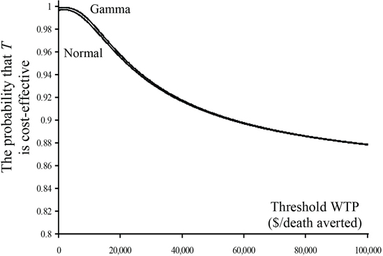
Estimates of the five parameters, ignoring any influence of the covariate, are given in Table 15.2. The estimates in the first column are derived from the formulae given in Section 15.3.2.1 using the pooled formulae for the variance and covariance. The estimates in the second column are derived from specifically modeling cost using a normal distribution. See Program 15.1 for details. As expected, the estimates in this column are almost identical to the estimates in the first. The estimates in the third column are derived from modeling cost using a gamma distribution. See Program 15.2 for details. Although the estimates of the Δ_e and Δ_c are very similar to those in the first two columns, the estimate of variance of $V\left({\hat{\mathrm{\Delta }}}_c\right)$ is more than 25% smaller, indicating that the gamma distribution provides a much better fit of the data. The impact of this increase in efficiency is demonstrated in Figures 15.7 and 15.8. Plots of the estimates and confidence limits of b_λ, as a function of λ, are given in Figure 15.7 for both the normal and gamma model assumptions. The CEACs are given in Figure 15.8. Although the gamma model provides a significant decrease in the variance of the estimated difference in mean cost, the confidence limits for the INB for the normal and gamma models are essentially equivalent, especially for values of λ that are appropriate for preventing a death. Some separation can be seen in the plot of the CEACs for low values of λ, but the curves are indistinguishable for larger, more appropriate values.

The following SAS code provides the estimates of the five required parameters, where arm is the treatment group indicator (1 for T and 0 for S), effectiveness equals 1 if the patient survived 30 days and 0 otherwise, and cost is the total cost for each patient.

Program 15.1 Modeling Cost Using a Normal Distribution

proc genmod data=yourDataset;
   model cost = arm / dist=normal link=identity;
   output out=c predicted=pred_c;
run;

proc genmod data= yourDataset desc;
   model effectiveness= arm / dist=bin link=identity;
   output out=e predicted=pred_e;
run;

data temp; merge e c;
   resid_e = effectiveness - pred_e;
   resid_c = cost - pred_c;
   keep resid_e resid_c;
run;

proc corr data=temp; var resid_e resid_c; run;

 

Output from Program 15.1

The following SAS code provides the estimates of the five required parameters. The output (not shown) has the same structure as the Output from Program 15.1.

Program 15.2 Modeling Cost Using a Gamma Distribution

proc genmod data=yourDataset;
   model cost = arm / dist=gamma link=identity;
   output out=c predicted=pred_c;
run;

proc genmod data= yourDataset desc;
   model effectiveness= arm / dist=bin link=identity;
   output out=e predicted=pred_e;
run;

data temp; merge e c;
   resid_e = effectiveness - pred_e;
   resid_c = cost - pred_c;
   keep resid_e resid_c;
run;

proc corr data=temp; var resid_e resid_c; run;

 

Table 15.2 Parameter Estimates for the CD Trial

Parameter	Pooled	Normal*	Gamma*
${\hat{\mathrm{\Delta }}}_e$	0.0507	0.0507	0.0507
${\hat{\mathrm{\Delta }}}_c$	−805.72	−805.72	−805.72
$\hat{V}\left({\hat{\mathrm{\Delta }}}_e\right)$	0.0002506	0.0002496	0.0002496
$\hat{V}\left({\hat{\mathrm{\Delta }}}_c\right)$	88,828	88,697	65,839
$\hat{C}\left({\hat{\mathrm{\Delta }}}_e,{\hat{\mathrm{\Delta }}}_c\right)$	−1.482	−1.473	−1.268

* distribution used for cost

Figure 15.7 Incremental Net Benefit and Confidence Limits Using the Normal and Gamma Distributions for the CD Trial

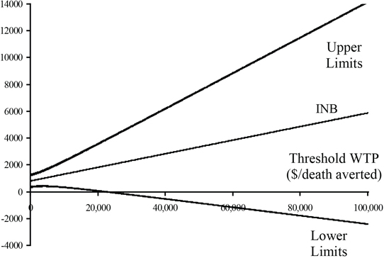
Figure 15.8 Cost-Effectiveness Acceptability Curves Using the Normal and Gamma Distributions for the CD Trial

Using a gamma distribution for cost, we examined the effect of the covariate on cost and 30-day survival. There was no significant effect (p = 0.5843) of the covariate on 30-day survival, but there was a significant overall affect (0.0315) and a marginally significant interaction (0.0630) with treatment group for cost. Final models, which include treatment group, X, and the interaction for cost and treatment group only for 30-day survival, were used to provide parameter estimates. See Program 15.3 for details. The parameter estimates are given in Table 15.3. Because of the interaction term between treatment group and X for the cost model, estimates of Δ_c and the associated variance and covariance depend on the level of X. The cost saving is much higher for X = 0, and consequently treatment will be more cost-effective in that subgroup of patients. The plot of incremental net benefit and the CEAC are given in Figures 15.9 and 15.10. The CEAC exceeds 0.9 for X = 0 for all values of λ, and it exceeds 0.85 for X = 1 for values of λ greater than $10,000 per life saved. This provides strong evidence in support for the cost-effectiveness of T.

A Microsoft EXCEL file for generating the plots of the CEAC and the INB (with confidence intervals) is available at http://www.andywillan.com/downloads. The only inputs required are the five parameter estimates, the minimum and maximum values for λ and the confidence level.

The following code shows the final models. The model for effectiveness included arm as the only covariate and the model for cost included arm, X, and their interaction.

Program 15.3 Covariate Adjustment

Program 15.3  Covariate Adjustment
proc genmod data=yourData;
   model cost = arm X arm*X/ dist=gamma link=identity;
   output out=c predicted=pred_c;
run;

proc genmod data=yourData desc;
   model effectiveness = arm / dist=bin link=identity;
   output out=e predicted=pred_e;
run;

data temp; merge e c;
   resid_e = effectiveness - pred_e;
   resid_c = cost - pred_c;
   keep resid_e resid_c;
run;

proc corr data=temp; var resid_e resid_c; run;

 

Output from Program 15.3

For X = 0: ${\hat{\mathrm{\Delta }}}_c=$ −1226.95; $\hat{V}\left({\hat{\mathrm{\Delta }}}_c\right)=$ (360.0549)².

For X = 0: $\hat{C}\left({\hat{\mathrm{\Delta }}}_e,{\hat{\mathrm{\Delta }}}_c\right)=$ (−0.31470)* (360.0549)*(0.0158).

For parameter estimates for X = 1, the values of X can be reversed and the program rerun, yielding the following output:

For X = 1:${\hat{\mathrm{\Delta }}}_c=$ −227.89; $\hat{V}\left({\hat{\mathrm{\Delta }}}_c\right)=$(361. 9759)².

For X = 1: $\hat{C}\left({\hat{\mathrm{\Delta }}}_e,{\hat{\mathrm{\Delta }}}_c\right)=$ (−0.31470)* (361.9759)*(0.0158).

Table 15.3 Parameter Estimates by Levels of the Covariate for the CD Trial

Parameter	X = 0	X = 1
${\hat{\mathrm{\Delta }}}_e$	0.0507	0.0507
${\hat{\mathrm{\Delta }}}_c$	−1226.95	−277.89
$\hat{V}\left({\hat{\mathrm{\Delta }}}_e\right)$	0.002496	0.0002496
$\hat{V}\left({\hat{\mathrm{\Delta }}}_c\right)$	129,640	131,027
$\hat{C}\left({\hat{\mathrm{\Delta }}}_e,{\hat{\mathrm{\Delta }}}_c\right)$	−1.790	−1.800

Figure 15.9 Incremental Net Benefit by Levels of the Covariate for the CD Trial

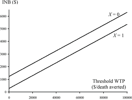
Figure 15.10 Cost-Effectiveness Acceptability Curves by Levels of the Covariate for the CD Trial

 

15.5 Observational Studies

Although many cost-effectiveness analyses are performed on data from randomized clinical trials, the methods are also appropriate for the comparison of two groups from observational studies, subject to the concerns one might have regarding bias due to the lack of random group allocation. Typically, an analysis for comparing two groups based on data from an observational study requires adjustment for selection bias. Two general approaches are available: propensity scoring and regression analysis. If the data set is sufficiently large, then propensity matching is a possible option (see Chapter 3). In this case, the propensity match data could be analyzed as if they came from an RCT. Propensity stratification is also an option (see Chapter 2). For propensity stratified data, a regression analysis is required, where effectiveness and cost must be regressed on the treatment indicator variable plus the dummy indicator variables for the propensity stratification (one less than the number of strata). For non-censored data, the analyst can use PROC GENMOD to perform the regression, as demonstrated in the example in Section 15.4. The stratification variable can be included in the CLASS statement, negating the need to create the dummy indicators. For censored data, the regression methods given in Willan, Lin, and Manca (2005) are appropriate. For regression analysis without propensity stratification, refer to Willan, Briggs, and Hoch (2004) for non-censored data and to Willan, Lin, and Manca (2005) for censored data.

 

15.6 Discussion

Outlined in this chapter is the use of the incremental net benefit for comparing the cost-effectiveness of two groups. An analyst can, as a function of the threshold WTP, estimate the INB and determine its corresponding confidence limits in a Frequentist’s approach or, alternatively, in a Bayesian approach plot the cost-effectiveness acceptability curve. The CEAC has the advantage that it both displays the magnitude of the estimated between-group contrast and characterizes its uncertainty. The INB is preferred to the ICER, which suffers from all the problems associated with ratio statistics. Further, the INB ties in directly with Bayesian decision analysis and is used in value of information methods (see, for example, Willan and Pinto, 2006, and other sources under “References”). As with other cost-effectiveness analyses, inference focused on INB requires the estimation of the between-group differences in mean effectiveness and mean cost. In addition, the variances and covariance of these estimators are required. The methods used for parameter estimation depend on

• whether censoring is present

• whether covariates are adjusted for

• whether random effects such as center or country are accounted for

• what the assumptions are regarding the distribution for cost

For situations where there is no censoring, covariates, or random effects and the skewing of cost data is ignored, only simple statistics are required. SAS PROC GENMOD can be used to accommodate covariates and random effects and specify skewed distributions for modeling costs. The presence of censoring adds an additional layer of complexity and is covered elsewhere (for example, Willan and Briggs, 2006; Willan et al., 2002; Willan et al., 2003; and so forth).

 

Acknowledgments

The author is funded through the Discovery Grant Program of the Natural Sciences and Engineering Research Council of Canada (grant number 44868−03).

 

References

Bang, H., and A. A. Tsiatis. 2000. “Estimating medical costs with censored data.” Biometrika 87(2): 329–343.

Briggs, A. H., and A. M. Gray. 1998. “The distribution of health care costs and their statistical analysis for economic evaluation.” Journal of Health Services Research & Policy 3(4): 233–345.

Briggs A. H., D. E. Wonderling, and C. Z. Mooney. 1997. “Pulling cost-effectiveness analysis up by its bootstraps; a non-parametric approach to confidence interval estimation.” Health Economics 6(4): 327–340.

Briggs, A., R. Nixon, S. Dixon, and S. Thompson. 2005. “Health economics letter: parametric modeling of cost data: some simulation evidence.” Health Economics 14: 421–428.

Chaudhary, M. A., and S. C. Stearns. 1996. “Estimating confidence intervals for cost-effectiveness ratios: an example from a randomized trial.” Statistics in Medicine 15: 1447–58.

Cochran, W. G. 1997. Sampling Techniques. New York: John Wiley & Sons, Inc.

Cook, J. R., M. Drummond, H. Glick, and J. F. Heyse. 2003. “Assessing the appropriateness of combining economic data from multinational clinical trials.” Statistics in Medicine 22: 1955–76.

Eckermann, S., and A. R. Willan. 2007. “Expected value of information and decision making in HTA.” Health Economics 16: 195–209.

Eckermann, S., and A. R. Willan. 2008. “The option value of delay in health technology assessment.” Medical Decision Making 28(3): 300–305.

Eckermann, S., and A. R. Willan. 2008. “Time and expected value of sample information wait for no patient.” Value in Health 11(3): 522–526.

Eckermann, S., and A. R. Willan. 2009. “Globally optimal trial design for local decision making.” Health Economics 18:203–216.

Efron, R. B., and B. R. J. Tibshirani. 1993. An Introduction to the Bootstrap. New York: Chapman & Hall.

Fenwick, E., B. J. O’Brien, and A. H. Briggs. 2004. “Cost-effectiveness acceptability curves––facts, fallacies and frequently asked questions.” Health Economics 13: 405–415.

Grieve, R., R. Nixon, S. G. Thompson, and C. Normand. 2005. “Using multilevel models for assessing the variability of multinational resource use and cost data.” Health Economics 14: 185–196.

Lin, D.Y. 2000. “Linear regression analysis of censored medical costs.” Biostatistics 1:35–47.

Lin, D. Y., E. J. Feuer, R. Etzioni, and Y Wax. 1997. “Estimating medical costs from incomplete follow-up data.” Biometrics 53: 419–34.

Lumley, T., P. Diehr, S. Emerson, and L. Chen. 2002. “The importance of the normality assumption in large public health data sets.” Annual Review of Public Health 23: 151–169.

Manca, A., N. Rice, M. J. Sculpher, and A. H. Briggs. 2005. “Assessing generalisability by location in trial-based cost-effectiveness analysis: the use of multilevel models.” Health Economics 14: 471–475.

Manning, W. G., and J. Mullahy. 2001. “Estimating log models: to transform or not to transform?” Journal of Health Economics 20: 461–94.

Nixon, R. M., and S. G. Thompson. 2004. “Parametric modeling of cost data in medical studies.” Statistics in Medicine 23: 1311–1331.

Nixon, R. M., and S. G. Thompson. 2005. “Methods for incorporating covariate adjustment, subgroup analysis and between-centre differences into cost-effectiveness evaluations.” Health Economics 14: 1217–1229.

O’Brien, B. J., K. Gertsen, A. R. Willan, and A. Faulkner. 2002. “Is there a kink in consumers’ threshold value for cost-effectiveness in health care?” Health Economics 11(2): 175–180.

O’Hagan, A., and J. W. Stevens. 2001. “A framework for cost-effectiveness analysis from clinical trial data.” Health Economics 10(4): 303–315.

O’Hagan, A., and J. W. Stevens. 2003. “Assessing and comparing costs: how robust are the bootstrap and methods based on asymptotic normality?” Health Economics 12(1): 33–49.

Pinto, E. M., A. R. Willan, and B. J. O’Brien. 2005. “Cost-effectiveness analysis for multinational clinical trials.” Statistics in Medicine 24: 1965–1982.

Thompson, S. G., D. E. Warn, and R. M. Turner. 2004. “Bayesian methods for analysis of binary outcome data in cluster randomized trials on the absolute risk scale.” Statistics in Medicine 23: 389–410.

Thompson, S. G., and J. A. Barber. 2000. “How should cost data in pragmatic randomised trials be analysed?” British Medical Journal 320(7243): 1197–1200.

Wilke, R. J., H. A. Glick, D. Polsky, and K. Schulman. 1998. “Estimating country-specific cost-effectiveness from multinational clinical trials. Health Economics 7(6): 481–493.

Willan, A. R. 2007. “Clinical decision making and the expected value of information.” Clinical Trials 4: 279–285.

Willan, A. R., A. H. Briggs, and J. S. Hoch. 2004. “Regression methods for covariate adjustment and subgroup analysis for non-censored cost-effectiveness data.” Health Economics 13: 461–475.

Willan, A. R., and D. Y. Lin. 2001. “Incremental net benefit in randomized clinical trials.” Statistics in Medicine 20: 1563–1574.

Willan, A. R., B. J. O’Brien, and R. A. Leyva. 2001. “Cost-effectiveness analysis when the WTA is greater than the WTP.” Statistics in Medicine 20: 3251–3259.

Willan, A. R., and A. H. Briggs. 2006. Statistical Analysis of Cost-effectiveness Data. West Sussex, England: John Wiley & Sons, Ltd.

Willan, A. R., and B. J. O’Brien. 1996. “Confidence intervals for cost-effectiveness ratios: an application of Fieller’s theorem.” Health Economics 5(4): 297–305.

Willan, A.R., D. Y. Lin, and A. Manca. 2005. “Regression methods for cost-effectiveness analysis with censored data.” Statistics in Medicine 24: 131–145.

Willan, A. R., D. Y. Lin, R. J. Cook, and E. B. Chen. 2002. “Using inverse-weighing in cost-effectiveness analysis with censored data.” Statistical Methods in Medical Research 11: 539–51.

Willan, A. R., E. B. Chen, R. J. Cook, and D. Y. Lin. 2003. “Incremental net benefit in randomized clinical trials with qualify-adjusted survival.” Statistics in Medicine 22: 353–62.

Willan, A. R., and E. M. Pinto. 2005. “The expected value of information and optimal clinical trial design.” Statistics in Medicine 24: 1791–1806.

Willan, A. R., E. M. Pinto, B. J. O’Brien, P. Kaul, R. Goeree, L. Lynd, et al. 2005. “Country-specific cost comparisons from multinational clinical trials using empirical Bayesian shrinkage estimation: the Canadian ASSENT−3 economic analysis.” Health Economics 14: 327–338.

Willan, A. R., and M. E. Kowgier. 2008. “Determining optimal sample sizes for multi-stage randomized clinical trials using value of information methods.” Clinical Trials 5: 289–300.

Willan, A. R. 2008. “Optimal sample size determinations from an industry perspective based on the expected value of information.” Clinical Trials 5: 587–594.

Zhao, H., and L. Tian. 2001. “On estimating medical cost and incremental cost-effectiveness ratios with censored data.” Biometrics 57: 1002–1008.