
Structural Nested Models
10.2 Time-Varying Causal Effect Moderation
10.4 Empirical Example: Maximum Likelihood Data Analysis Using SAS PROC NLP
This chapter reviews Robins’ Structural Nested Mean Model (SNMM) for assessing the effect of predictors that vary over time. The SNMM is used to study the effects of time-varying predictors (or treatments) in the presence of time-varying covariates that are moderators of these effects. We describe a SAS implementation of a maximum likelihood (ML) estimator of the parameters of an SNMM using PROC NLP. The proposed ML estimator requires correct model specification of the distribution of the primary outcome given the history of time-varying moderators and predictors, including proper specification of both the causal and non-causal portions of the SNMM. The estimator also relies on correct model specification of the observed data distribution of the putative time-varying moderators given the past. We illustrate the methodology and SAS implementation using data from a weight loss study. In the empirical example, we assess the impact of early versus later weight loss (or gain) on end-of-study health-related quality of life as a function of prior weight loss and time-varying covariates thought to be moderators of these effects.
Longitudinal randomized trials are now commonplace in clinical research. This, together with the growing number of health-outcomes databases and improved access to medical records for research purposes, has given rise to an abundance of data sets in which patients contribute measures on a large number of variables repeatedly over time. This wealth of longitudinal data, in turn, has allowed researchers to examine more varied and detailed scientific questions concerning, for example, the etiology of diseases or the different causal pathways through which behavioral and other medical interventions produce positive health effects. Due to the ample availability of longitudinal data, these questions often involve time-varying predictors or treatments of interest (in addition to possibly longitudinal outcomes). Because the primary time-varying predictors (or treatments) of interest—that is, the primary independent or right-hand side variables of interest—often are not (or, as in the case of this chapter’s motivating example, cannot be) randomized or directly manipulated by experimentation, empirical longitudinal studies of this sort are often termed observational studies.
The methodology we discuss in this chapter focuses on a particular type of question involving time-varying predictors (or treatments). Specifically, we are interested in conceptualizing and estimating scientific questions concerning time-varying causal effect moderation (Petersen et al., 2007; Almirall et al., 2009).
To illustrate, informally, what we mean by time-varying effect moderation, consider a simplification of our motivating example (described in more detail in Section 10.4) in which repeated measures of body weight (Zj) and a dichotomous time-varying covariate (Xj), exercise (yes/no), are available at multiple time points j (j = 0,1,2,…,T) over the course of a study. We define measures of body weight change between successive time points as Dj = Zj – Zj-1 (j=1, 2,…, T). Suppose our outcome is a health-related quality of life measure (QOL = Y), available at the end of study (at or after time T). Using these data, at each time point j we are interested in asking how the impact of weight loss or weight gain (Dj) on end-of-study health-related quality of life (Y) differs as a function of the history of exercise through time j-1. In other words, we are interested in the effect of Dj on Y as a function of (X0, X1,…, Xj-1). Thus, by time-varying causal effect moderation we refer to the way in which the time-varying covariate exercise moderates (changes, tempers, or modifies) the causal effects of the time-varying predictor weight loss or weight gain on end-of-study health-related quality of life (HRQOL).
In our motivating example, identifying and understanding time-varying moderators of the effect of weight change on health-related quality of life is important because it enhances our understanding of the causal pathways by which weight loss (or gain) leads to improved (or decreased) health-related quality of life. The process also can help us to better appreciate the relationship among the outcome (HRQOL), time-varying moderators (for example, exercise), and factors that do not vary with time but may moderate both the outcome and the time-varying moderators. Examples of these factors include patient characteristics (for example, demographics, medical diagnoses) and weight loss intervention type (for example, diet composition, weight loss medication, bariatric surgery) or structure (for example, visit frequency, individual vs. group sessions). This specified knowledge can be used to corroborate old hypotheses or to generate new ideas about the relationships among weight loss, health-related quality of life, and time-varying moderators of both weight loss and HRQOL, including exercise or adherence to the intervention. This additional knowledge, in turn, may help clinicians predict the positive health effects of weight loss given current knowledge about a patient’s exercise behavior and/or adherence to diet. It may also serve as a guide that behavioral scientists can use to help develop future interventions for weight loss or body weight management.
In linear regression models, effect moderation (or effect modification) is typically associated with interaction terms between the primary predictor variable and the covariate (or putative moderator) of interest. For example, in the point-predictor setting in which the primary predictor D, weight change, and the covariate of interest, X, do not vary over time, the following regression model could be used to study effect moderation:
E(Y | X, D) = γ0 + γ1X + γ2D + γ3DX (1)
In this model, the cross-product term quantifies the extent to which the impact of D on Y varies according to levels of X. That is, a one-unit increase in weight change corresponds to a γ2 + γ3X unit change in health-related quality of life at the end of the study, which differs by the levels of X, exercise (yes/no). Thus, in this model, γ3 = 0 is evidence that there is no effect moderation by X, or exercise level.
Unfortunately, this regression modeling strategy does not translate straightforwardly to the time-varying setting. Consider the following extended model for the time-varying setting where T = 2:
E(Y | X0, D1, X1, D2) = γ0 + γ1X0 + γ2D1 + γ3D1X0 + γ4X1 + γ5D2 + γ6D2X1 + γ7D2X0 + γ8X0X1 (2)
In this model, X0 is exercise level prior to baseline (j=0), X1 is exercise level between time j=0 and time j=1, D1 is weight change between baseline (j=0) and time j=1, and D2 is weight change between time j=1 and time j=2. Even if (2) is the correct model (that is, the correct functional form) for the conditional expectation (association) of Y given (X0, D1, X1, D2), the parameters associated with the D1 and the D1X0 cross-product terms may not necessarily represent the conditional causal effect of weight change D1 on end-of-study quality of life Y within levels of exercise X0. That is, the function γ2 + γ3X0 may or may not represent the true conditional causal effect of unit changes in weight change (between baseline and j = 1) on end-of-study quality of life.
The problem with naively extending the cross-product modeling strategy to the time-varying setting, as in (2), is that it is not clear what causal effects, if any, the coefficients of D1 and D1X0 in (2) are measuring. The main source of the problem (for causal inference) is that model (2) conditions on X1 (exercise level between time j=0 and j=1), which is likely affected by D1, weight loss or weight gain between time j=0 and time j=1 (Robins, 1987, 1989, 1994, 1997, 1999a; Bray et al., 2006). This has two undesirable consequences. First, naively conditioning on X1 cuts off any portion of the effect of weight change (D1) on Y that is transmitted using X1; that is, the function γ2 + γ3X0 does not include the effects (including effect moderation by X0) of D1 on Y that are mediated (Baron and Kenny, 1986; Kraemer et al., 2001) by X1. Second, naively conditioning on X1 introduces bias in the coefficients (γ2, γ3) due to nuisance associations between X1 and Y that are not on the causal pathway between D1 and Y. These include nuisance associations due to variables that are related to both X1 and Y. Thus, while the scientist wishes to condition on the time-varying covariate X because of interest in X’s role as a time-varying moderator of the effect of time-varying D on Y, doing so in the traditional way (that is, using standard regression adjustment) is not suitable because of the potential for bias.
Robins’ Structural Nested Mean Model (1994) overcomes these problems by clearly specifying the causal and non-causal portions of the conditional mean of Y given the past (the history of weight change and time-varying moderators). The SNMM clarifies the meaning of causal effect moderation when both primary predictors of interest and putative moderators are time varying. The SNMM serves as a guide for properly incorporating potential time-varying moderators in the linear regression.
In Section 10.2 we define, more formally, what is meant by time-varying effect moderation in the context of a causal model for the conditional mean of the outcome given the past (that is, using Robins’ SNMM). In Section 10.3 we describe a maximum likelihood (ML) estimator of parameters of the SNMM. In Section 10.4, we demonstrate a SAS PROC NLP implementation of the ML estimator using real data from a weight loss study. In the empirical example, we assess the impact of early versus later weight loss (or gain) on end-of-study vitality (a health-related quality of life measure) as a function of prior weight loss and time-varying covariates (exercise, diet adherence, and prior vitality scores) thought to be moderators of these effects.
10.2 Time-Varying Causal Effect Moderation
10.2.1 Notation
We rely on the potential outcomes notation to define the causal parameters of interest (Rubin, 1974; Holland, 1986, 1990). As described briefly in the introduction, we consider the following general temporal data structure:
(X0, d1, X1(d1), d2,…, XT-1(d1, d2,…, dT-1), dT, Y(d1, d2,…, dT)). (3)
In this notation, dj (j = 1, 2,…, T) is an index for the primary time-varying predictor variable (for example, time-varying weight change) at time j. In our example, dj is the change in body weight defined as the difference between weight at the current visit (time j) and the previous visit (at time j-1). For instance, (d1, d2) = (-3, 0) denotes a loss of 3 pounds in body weight between the first and second visits and no change in body weight between the second and third visits. We use lowercase dj to distinguish it from the observed data predictors, which are random variables, denoted by uppercase Dj (see Section 10.3). Xj(d1, d2,…, dj) (j = 1,2,…,T-1), possibly a vector, denotes the time-varying covariate(s) (the putative time-varying moderator(s) of interest) at time j. X0 may include assignment to a diet type or structure, baseline patient traits, characteristics, or demographics (such as age, race, gender, and income), as well as baseline measures of the time-varying covariates. We impose no restriction on the type of time-varying covariates considered; Xj(d1, d2,…, dj) and X0 may be continuous or categorical. Finally, Y(d1, d2,…, dT) denotes the potential outcome at the end of the study (that is, occurring after dT ; for example, end-of-study health-related quality of life). In this chapter, we consider only continuous, unbounded outcomes Y. For example, Y(d1, d2,…, dT) is the outcome a patient would have had had they lost (or gained) weight over the course of the study in increments (decrements) of (d1, d2,…, dT) . That is, Y(d1, d2,…, dT) describes the end-of-study outcome under a particular trajectory or course of weight loss or gain. Note that in our notation, Xj(d1, d2,…, dj) (j = 1,2,…,T-1) are also indexed by dj because they are potentially affected by prior levels of dj. That is, they are also conceived as potential outcomes. Indeed, the vector of time-varying covariates may include prior time-varying instances of the primary outcome variable Y(d1, d2,…, dT) . For instance, in the context of our motivating example, prior levels of quality of life may also moderate the future impact of weight loss on end-of-study quality of life.
We use the underscore notation as short-hand to denote the history of a variable or index, as follows:
dj = (d1, d2,…, dj);
Xj(dj) = (X0, X1(d1), X2(d2), …, Xj(dj)); and
Y(dT) = Y(d1, d2,…, dT) .
In this chapter, we do not consider longitudinal outcomes; we consider only outcomes measured at the end of the study (post-dT). Therefore, we do not index the outcome Y(dT) by a subscript denoting time. It is possible, however, to extend the methods presented here to handle longitudinal outcomes (Robins, 1994).
10.2.2 Robins’ Structural Nested Mean Model
In this subsection, we define our primary causal functions of interest in the context of Robins’ SNNM. In general, there are T causal effect functions of interest, one per time point. For simplicity, we present the SNMM in the simple T = 2 post-baseline (meaning, post-X0) time points setting. Thus, we have the following objects to define our causal effects with:
(X0, d1, X1(d1), d2, Y(d1, d2)).
The first causal effect is denoted by
μ1(X0 ,d1) = E (Y(d1, 0) – Y(0, 0) | X0). (4)
μ1(X0 ,d1) is the average causal effect of (d1,0) versus (0,0) on the outcome conditional on X0. In the context of our motivating example, μ1(X0 ,d1) represents the causal effect on end-of-study health-related quality of life of having lost (or gained) d1 pounds between the first and second visits to the clinic and no change in weight thereafter (Y(d1, 0)) versus no change in weight during the entire study (Y(0, 0)), as a function of X0, baseline exercise and/or other demographic characteristics that are a part of X0.
The second causal effect is defined as
μ2(X1(d1),d2) = E (Y(d1,d2) – Y(d1,0) | X1(d1)), (5)
which is the average causal effect of (d1,d2) versus (d1,0) on the outcome, conditional on both X0 and X1(d1). In the context of our motivating example, μ2(X1(d1),d2) represents the causal effect on end-of-study health-related quality of life of having lost (or gained) d2 pounds between the second and third visits to the clinic (Y(d1,d2)) versus no change in weight between the second and third visits to the clinic (Y(d1,0)) as a function of both X0 and X1(d1), and supposing a change in weight of d1 between the first and second clinic visits.
In our example, then, μ1(X0 ,d1) captures the effect of losing (or gaining) weight early on in the study and not losing any weight thereafter, whereas, μ2(X1(d1),d2) captures the effect of losing (or gaining) weight later on in the study. In addition, by conditioning on the history of time-varying covariates, these functions allow us to model the average effect of losing weight early versus later while taking into account changing patterns in the evolving state of patients in terms of Xj (for example, exercise).
Robins’ SNMM is a particular additive decomposition of the conditional mean of Y(d1,d2) given X1(d1) that includes the functions μ1(X0 ,d1) and μ2(X1(d1),d2) as part of the decomposition. Specifically, for T = 2 the SNMM can be written as follows:
E (Y(d1,d2) | X1(d1)) = β0 + ε1(X0) + μ1(X0 ,d1) + ε2(X1(d1)) + μ2(X1(d1),d2), (6)
where β0 is the intercept equal to E (Y(0,0)) , which is the mean outcome under no weight gain or loss during the course of the study. The functions ε1(X0) and ε2(X1(d1)) are defined to make the right-hand side of (5) equal the conditional mean of Y(d1,d2) given X1(d1). That is, the functions ε1(X0) and ε2(X1(d1)) are defined as follows:
ε1(X0) = E (Y(0,0) | X0) – E (Y(0,0)) (7)
ε2(X1(d1)) = E (Y(d1,0) | X1(d1)) – E (Y(d1,0) | X0) (8)
We label the functions ε1(X0) and ε2(X1(d1)) as nuisance functions to distinguish them from our primary causal functions of interest, μ1(X0 ,d1) and μ2(X1(d1),d2). They connote both causal and non-causal relationships (associations) between the time-varying moderators and the outcome Y.
The components of the SNMM exhibit two properties, which dictate how we model these quantities:
First, we note that μj = 0 whenever dj = 0. (9)
Second, the nuisance functions are mean-zero functions conditional on the past: (10)
E (εj(Xj-1(dj-1)) | Xj-2) = 0.
Thus, in the T = 2 time points setting, for instance:
a. E (ε1(X0)) = 0, where the expectation is over the X0 random variable(s), and
b. E (ε2(X1(d1)) | X0 ) = 0,where the expectation is over the X1(d1) random variable(s) conditional on X0.
Property (9) makes sense because causal effects should be 0 when comparing the same course of weight change over time, regardless of covariate history. Property (10) is what makes the SNMM a non-standard regression model because it is a function of conditional mean-zero error terms. Intuitively, ε2(X1(d1)) captures the mean association between Y(d1,0) and having more (X1(d1)) versus less (X0) covariate information. Property (10) indicates that this information deficit can be expressed as a function of the mean residual information in X1(d1) not explained by d1 and X0 (which has mean zero). Recognition of the nuisance functions in the model for E(Y(d1,d2) | X1(d1)) is what makes the SNMM distinct from the standard regression model shown in (2). Further, understanding how to model the nuisance functions properly helps resolve the challenges with the standard regression model (2) that were discussed in the Introduction.
10.3.1 Observed Data and Causal Assumptions
Section 10.2.1 introduced the potential outcomes that were used to define the causal parameters of interest. In this section, we describe the observed data—and their connection to the potential outcomes—which are used to estimate the causal parameters of interest. Let Dj denote the observed value of the primary time-varying predictor of interest at time j; and let Dj = (D1, D2,…,Dj) denote the history of the observed time-varying predictor through time j. Let Xj (possibly a vector) denote the observed value of the time-varying covariate (or potential moderator) at time j, and let Xj = (X1 , X2,…, Xj). Let Y denote the observed end-of-study outcome. The full set of observed data, O, has the following temporal order:
O = (X0, D1, X1, D2,… , XT-1, DT, Y). (11)
The connection (link) between the potential outcomes in (2) and the observed data in (11) is established by invoking the Consistency Assumption (Robins, 1994) for both the observed time-varying covariates and the observed end-of-study outcome Y. For all subjects in the study, the Consistency Assumption for the end-of-study outcome states that
Y = Y(DT), (12)
where the right-hand side Y(DT) denotes the potential outcome indexed by values of dT equal to DT. Intuitively, this assumption states that the observed outcome Y for a subject that follows the trajectory of observed primary predictor values DT agrees with the potential outcome indexed by the same trajectory of values. Note that the observed potential outcome Y = Y(DT) is just one of many potential outcomes that could have been observed. Similarly, we assume consistency for each of the potential putative time-varying moderators in XT-1(dT-1), to link them up with the observed values XT.
In order to estimate the values of μj using the observed data, we also assume the No Unmeasured (or Unknown) Confounders Assumption (Robins, 1994):
For every j (j = 1,2,…,T), Dj is independent of (Y(dT) for all dT) conditional on Xj-1. (13)
Intuitively, this untestable assumption states (for every j) that aside from the history of putative time-varying moderators up to time j, there exist no other variables (measured or unmeasured, known or unknown) that are directly related to both Dj and the potential outcomes. Together with the Consistency Assumption, the No Unmeasured Confounders Assumption allows us to draw causal inferences from observed differences in the data (see Supplementary Web Appendix B in Almirall et al., 2009).
10.3.2 Parametric Models for the Components of the SNMM: Modeling Assumptions
Properties (9) and (10) serve as a guide for parametric models for the causal and non-causal portions of the SNMM. In this chapter, we consider simple linear parametric models for the values of μj such as the following:
μj(Xj-1,Dj; βj) = Dj(βj0 + βj1 Xj-1) = βj0 Dj + βj1 Dj Xj-1, (14)
where βj = (βj0, βj1) is an unknown column vector of parameters. This model, for example, implies that the effect of a unit change in D1 (for example, weight change between baseline and t = 1) on the outcome varies linearly in Xj-1 with slope equal to βj1.
Assume for the moment that Xj-1 is univariate for all j. For each εj, j = 1, 2,…,T, we consider parametric models for the nuisance functions such as the following:
εj(Xj-1, Dj-1 ; λj, ηj) = δj(Xj-1, Dj-1; ηj) λj (15)
where ηj is an unknown scalar parameter. More complex forms—where the εj’s are indexed by a row vector of unknown parameters ηj—are discussed in Almirall and colleagues (2009). The residual δj is equal to Xj-1 - mj(Xj-2,Dj-1; λj), where mj(Xj-2,Dj-1; λj) = gj(Fjλj) is a general linear model (GLM), with link function gj(), for the conditional expectation E(Xj-1 | Xj-2,Dj-1) based on the unknown parameters λj. For binary Xj-1, gj() can be either the inverse logit transform or the inverse probit transform. On the other hand, if Xj-1 were continuous, then gj() would be the identity function. Note that E(δj(Xj-1, Dj-1; λj) | Xj-2,Dj-1) = 0 by definition.
As an example, suppose Xj is a binary indicator of exercise measured at time j. In this case, a sample model for εj is εj(Xj-1, Dj-1 ; ηj, λj) = (Xj – pj(λj)) ηj, where pj(λj) is the predicted probabilities of a logistic regression of Xj on the past.
The parameterization shown in (15) ensures that models for the nuisance functions satisfy the constraint in (10). Observe that since E(δj(Xj-1, Dj-1; λj) | Xj-2,Dj-1) = 0, then E(εj(Xj-1, Dj-1 ; ηj, λj) | Xj-2,Dj-1) = E(δj(Xj-1, Dj-1; λj) ηj | Xj-2,Dj-1) = E(δj(Xj-1, Dj-1; λj) | Xj-2,Dj-1) ηj = 0.
The parameterization shown in (15) assumes that each Xj is univariate. For multivariate Xj (say, Xj = (Xjk :k = 1, 2,…, sj) , a vector of sj covariates at time j), we propose modeling the separate εjk’s for each Xjk as in (15) and then summing them together to create a model for jth time-point nuisance function εj.
Let β denote the full collection of parameters in the μj’s, including the SNMM intercept β0; and let η and λ denote the collection of parameters in the nuisance functions of the SNMM. Note that the parameters λ are shared between the SNMM and the conditional mean models for the time-varying covariates given the past. Next, we describe maximum likelihood estimation of the causal parameters (β) and non-causal (nuisance) parameters (η, λ) of the SNMM.
10.3.3 Maximum Likelihood Estimation
Recall that the full observed data for one person are denoted by O. The probability density function fO of the observed data O can be written as a product of conditional densities, as follows:
fO (O) = fY(Y | XT-1, DT) fj(Xj | Xj-1, Dj-1) f0(X0) πj(Dj | Xj-1, Dj-1), (16)
where fY is the conditional density of Y given (XT-1, DT), fj is the conditional density of Xj given (Xj-1, Dj-1), f0(X0) is the density of X0, and πj is the conditional density of Dj given (Xj-1, Dj-1).
In this chapter we assume that the conditional distribution of Y given (XT-1, DT) follows a normal distribution with conditional mean structure following an SNMM with parameters (β, η, λ) and residual square-root variance σY. Thus, fY is assumed to be a normal probability density function with parameters (β, η, λ, σY). The form of the conditional densities fj and f0 depend on the type of time-varying covariates found in the data. In our data example here, we encounter both continuous and binary random variables in XJ-1; for continuous time-varying covariates, we assume normality, whereas for binary time-varying covariates, we assume a Bernoulli distribution with conditional probability modeled by the logistic transform. In general practice, the quantity fj(Xj | Xj-1, Dj-1) f0(X0) may be a mixture of continuous and categorical conditional probability density functions. In any case, fj(Xj | Xj-1, Dj-1) f0(X0) is at least a function of λ, the unknown parameters indexing models for the expectation (mean) of Xj given the past. This is important because it means that the parameters λ are shared between the conditional density for Y given the past and other portions of the multivariate distribution of O. This happens because models for the conditional mean of the time-varying covariates are employed in the nuisance functions—that is, the εj’s—of the SNMM. The densities fj and f0 may also be a function of other variance components (for example, σj and σ0, if there are continuous time-varying covariates assumed to follow a normal distribution).
Let θ denote the full collection of unknown parameters in fY(Y | XT-1, DT) fj(Xj | Xj-1, Dj-1) f0(X0). Thus, θ includes (β, η, λ, σY) in fY, and λ and possibly other variance components (for example, σj and σ0) in fj(Xj | Xj-1, Dj-1) f0(X0).
To proceed with estimation of θ, we assume we have a data set, (O1, O2,…,ON), of N independent random variables, each assumed to be drawn from the distribution fO (O | θ). Therefore, written as a function of the unknown parameters θ, the complete data log-likelihood is
loglik1 = log fO (Oi | θ)
= (log fY (Yi | XT-1, i, DT, i; β, η, λ, σY) + log fj(Xj, i | Xj-1, i, Dj-1, i; (17)
λj, σj) f0(X0, i; λ0, σ0)
+ log πj(Dj, i | Xj-1, i, Dj-1, i)) ,
where i denotes subject i in the data set (i = 1, 2, …, N). Because the conditional distribution of Dj given (Xj-1, Dj-1) factorizes and is not a function of any of the parameters in θ, we can obtain a maximum likelihood (ML) estimate of θ by finding the value of θ that maximizes:
loglik2 = log fO (Oi | θ)
= (log fY (Yi | XT-1, i, DT, i; β, η, λ, σY) + log fj(Xj, i | Xj-1, i, Dj-1, i; (18)
λj, σj) f0(X0, i; λ0, σ0)) .
Denote the ML estimate of θ by . That is, = argmaxθ loglik2(θ).
The following section demonstrates how to estimate θ using ML with real data.
10.4 Empirical Example: Maximum Likelihood Data Analysis Using SAS PROC NLP
In this section, we demonstrate how to obtain ML estimates of the SNMM using SAS PROC NLP. Data for our illustrative example come from a randomized, controlled clinical trial comparing a low-carbohydrate (LC; NLC = 59) diet versus a low-fat diet (LF; NLF = 60) for weight loss, hereafter referred to as the LCLF Study (Yancy et al., 2004). Participants in both arms of the LCLF Study had measures of body weight, health-related quality of life (HRQOL), and exercise collected during clinic visits at baseline and every 4 weeks over the course of 16 weeks. In addition, adherence to diet was measured at every clinic visit post-baseline. Our total sample size is N = 119.
Using the LCLF Study data, Yancy and colleagues (2004) demonstrated improved weight loss, on average, for patients in the LC diet as compared with those following the LF diet, with most improvements in both arms of the study occurring during the first 12 weeks of study. Yancy and colleagues (2009) examined the effect of the LC diet versus the LF diet on a variety of quality of life measures and found that the LC diet group had greater improvements in the Mental Component Summary score of the Short Form 36 (SF-36), a commonly used and widely validated instrument for assessing HRQOL (McHorney et al., 1992; Ware and Sherbourne, 1992). In ongoing, unpublished research, we have also investigated the marginal impact of weight loss on quality of life using a Marginal Structural Model (MSM) (Robins, 1997, 1999a; Robins et al., 2000) and found some evidence that patients who lose weight faster enjoy a better intermediate and end-of-study health-related quality of life. Given these preliminary findings, we are also interested in better understanding the relationship among diet, weight loss, and quality of life, by studying the impact of weight change (that is, time-varying body weight) on health-related quality of life conditional on (that is, as modified by) the evolving state of the patient with respect to exercise, compliance with the diet, and prior levels of quality of life. While MSMs can be used to study the impact of time-varying weight loss, they cannot be used to study time-varying causal effect moderation (modification) because they do not allow conditioning on time-varying covariates.
10.4.1 Primary Scientific Question of Interest
In this chapter, we apply the SNMM to the LCLF data to study the extent to which assigned diet (LC versus LF), time-varying exercise, time-varying adherence to assigned diet, prior weight change, and prior levels of quality of life moderate the effect of losing (or gaining) weight early versus later over the course of 12 weeks on end-of-study vitality. In other words “do the effects of losing weight early versus later during the course of 12 weeks on end-of-study vitality scores differ depending on diet arm and time-varying covariates such as adherence to diet, exercise, and prior levels of quality of life?”
While our data arise from an experimental study, the causal effect moderation question we are interested in constitutes an observational study of the data because our primary right-hand side (or causal) variable of interest is longitudinal weight (change), which, unlike assignment to diet type (LC versus LF), cannot be manipulated experimentally.
10.4.2 Study Measures and Temporal Ordering
For our illustrative example, we are using LCLF Study data gathered at baseline and at clinic visits occurring every 4 weeks from baseline through week 16. Thus, for our purposes, there are five measurement occasions. In our study, the time-varying covariates of interest—measures of adherence to diet (COMPLY), exercise (EXER), and vitality (VIT)—are self-reported recollections designed to capture these constructs since the last visit or in the past 2 weeks. Thus, the time at which a measure is collected (clinic visits) is not necessarily the time at which the construct being measured actually occurred. In our causal analyses, therefore, we lag our measures appropriately to account for this feature of the data. We also do this acknowledging that in our conception of time-varying causal effect moderation in Section 10.2 we require that time-varying moderators Xj-1 occur prior to, or concurrent with, the primary predictor (or treatments) of interest at time j, Dj. In addition, the primary outcome Y must be measured at the end of the study, meaning after the occurrence of the final measure of the time-varying predictor, DT.
The first step in our data analysis, therefore, is to identify the primary measures of interest and their temporal ordering both in the data and in terms of the quantities they measure. Figure 10.1 summarizes the relationship among our study measures of interest, their timing in the LCLF Study, and how we use these measures in our data analysis.
Figure 10.1 Temporal Ordering of Study Measurements in LCLF Study
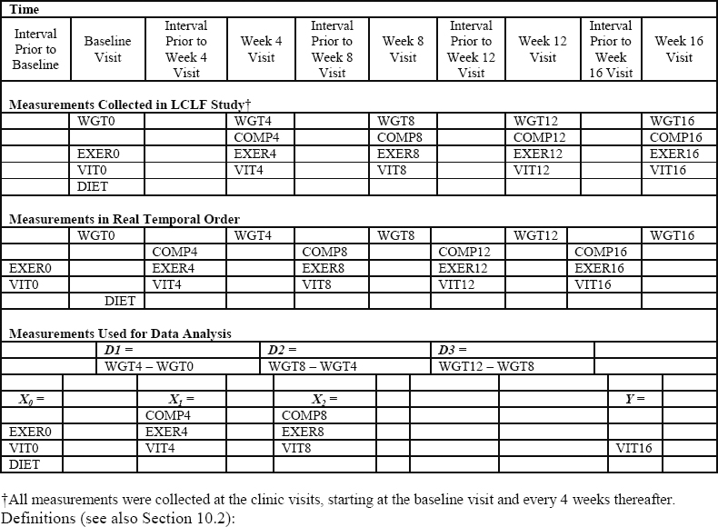
Definitions (see also Section 10.2):
DIET = diet type, a binary measure (1=LC diet; 0=LF diet)
WGT = weight, a continuous measure
COMP = adherence to diet, a binary measure
EXER = exercise, a binary measure
VIT = vitality (a quality of life outcome), a continuous measure
10.4.2.1 Primary Predictor of Interest: Successive Changes in Body Weight
Let Zj be the measure of body weight taken at visit j, where j = 0 denotes the baseline visit. Dj is defined as the difference in body weight between successive clinic visits: Dj = Zj – Zj-1. For our study, we consider measures of weight change over the course of 12 weeks post-baseline. Because clinic visits were 4 weeks apart, T = 3 (j = 1, 2, 3). Thus, we have D1 = weight change between baseline and the first clinic visit, D2 = weight change between the second and third clinic visits, and D3 = weight change between the third and fourth clinic visits.
10.4.2.2 Baseline and Time-Varying Moderators of Interest
The putative time-varying moderators (Xj-1: j = 1, 2, 3) include continuous time-varying measures of vitality (VIT0, VIT4, VIT8, respectively) and binary (yes/no = 1/0) time-varying indicators of self-reported exercise (EXER0, EXER4, EXER8, respectively). In addition, (X1, X2) include binary (yes/no = 1/0) indicators of compliance to diet between the baseline and the first visit (COMPLY4) and compliance to diet between the first and second visits (COMPLY8), respectively. In addition, X0 also includes a binary (LC/LF = 1/0) indicator of assigned diet arm (DIET).
We note that X0 does not include a compliance to diet measure because the diet arm was not assigned until the first clinic visit; therefore, compliance to diet is included only in (X1, X2). Technically, the diet arm was assigned immediately after the first body weight measure was taken at the baseline clinic visit. However, we can justify including DIET in X0 because diet assignment was randomized and, therefore, is unaffected by baseline levels of body weight (Z0). Further, it is sensible to ask whether the impact of body weight change between the baseline and the first follow-up clinic visit differs according to DIET.
10.4.2.3 Primary Outcome: Vitality
HRQOL is assessed using the Medical Outcomes Study SF-36 instrument (McHorney et al., 1992; Ware and Sherbourne, 1992), which measures HRQOL along eight dimensions of physical and mental health. The primary outcome measure for our analysis, Vitality, is one of the continuous physical HRQOL subscales derived from the SF-36 instrument. We use the Vitality component of the SF-36 for illustrating the SNMM methodology; however, we could have used one or more of the other HRQOL subscales, as well. Let Y = VIT16, a continuous measure of vitality during the interval of time just prior to the week 16 clinic visit. For illustrative purposes, we have restricted the outcome to be an end-of-study outcome, but the methods described in this chapter can be readily extended to handle a longitudinal outcome variable (Robins, 1994).
10.4.3 Parametric Models
For the conditional distribution of VIT16 given the past (that is, for fY), we assumed a normal distribution with residual square-root variance σY and conditional mean following a SNMM with this parameterization:
E (VIT16 | DIET, EXER8, VIT8, COMP8, D3) (19)
= β0 [intercept]
+ η14 δ1DIET + η15 δ1EXER0 + η16 δ1VIT0 [ε1(X0; η1)]
+ β10 D1 + β11 D1EXER0 + β12 D1VIT0 + β13 D1DIET [μ1(X0, D1; β1)]
+ η21 δ2COMPLY4 + η22 δ2EXER4 + η23 δ2VIT4 [ε2(X1, D1; η2)]
+ β20 D2 + β21 D2 EXER4 + β22 D2 VIT4 + β23 D2 COMPLY4 [μ2(X1, D2; β2)]
+ η31 δ3COMPLY8 + η32 δ3EXER8 + η33 δ3VIT8 [ε3(X2, D2; η3)]
+ β30 D3 + β31 D3 EXER8 + β32 D3 VIT8 + β33 D3 COMPLY8 [μ3(X2, D3; β3)]
The μj models in this SNMM are Markovian in the sense that each model for the effect of Dj on Y is only a function of prior weight change and measures of the time-varying covariates immediately preceding Dj. More complicated models could also be considered—for instance, models that allow the full history of time-varying covariates Xj-1 to moderate the impact of subsequent weight change on vitality.
Because EXER, COMPLY, and DIET are binary, we assume Bernoulli distributions for their conditional distributions given the past (that is, the fj’s), with probabilities modeled using logistic link functions (that is, g = inverse logit link). For example, for COMPLY4, the Bernoulli likelihood takes the form
f COMPLY4 = pCOMPLY4 (COMPLY4) + (1-pCOMPLY4) (1-COMPLY4),
where pCOMPLY4 denotes the predicted probability that COMPLY4 = 1 from a logistic regression of COMPLY4 on covariates (EXER0, VIT0, DIET, and D1). (See Section 10.4.4.2 for the corresponding SAS PROC NLP code.) For baseline (VIT0) and follow-up (VIT4, VIT8), which are continuous time-varying variables, we assume normal distributions for their conditional distributions with residual square-root variance σVIT0, σVIT4, and σVIT8 respectively (with g = identity function). In terms of the specific form of the linear portion of the GLMs (that is, models for the Fjλj), all models for the post-baseline variables included main effects for the history of covariates that preceded it and first-order interactions with prior levels of weight change, whereas for the baseline covariates, we use intercept-only models.
10.4.4 SAS PROC NLP
The NLP procedure in SAS provides a powerful set of optimization tools for minimizing or maximizing multi-parameter non-linear functions with constraints, such as our loglik2 (Property [18]). Recall from Property (18) that the complete data log-likelihood is a function of fY and fj and the parameters θ. In this parameterization, θ includes (β, η, λ, σY and λ) and possibly other variance components (for example, σj and σ0) depending on the distribution of the time-varying covariates that are used. Here we demonstrate how to use PROC NLP to find the value of the parameters in θ that maximize loglik2(θ). PROC NLP is particularly well-suited for this application because the log-likelihood function loglik2 is both non-linear in θ, and it includes simple inequality constraints. Specifically, the vector of parameters λ appears in the fY portion of the log-likelihood as a multiplicative product with parameters in η, and λ also appears in other portions of the log-likelihood. In addition, we constrain the variance components (for example, σY) in loglik2 to be positive.
We begin by inputting our data set into SAS and printing the data to ensure they were loaded correctly:
libname lib1 'My DocumentsWeightData';
proc print data=lib1.weight_data;
var subject diet exer0 vit0 d1 comply4 exer4 vit4 d2 comply8 exer8 vit8 d3 vit16;
run;
We show the first 12 lines of data here. The outcome is VIT16. DIET, EXER0, and VIT0 are baseline moderators of interest; D1 is weight change between baseline and week 4; COMPLY4, EXER4 and VIT4 are week 4 moderators; D2 is weight change between week 4 and week 8; COMPLY8, EXER8, and VIT8 are week 8 moderators of interest; and D3 is weight change between week 8 and week 12.
Output 10.1 SAS PROC NLP Analysis Data Set
| Obs | subject | DIET | exer20 | VIT0 | D1 | comply4 | exer24 | VIT4 | D2 | comply8 | exer28 | VIT8 | VIT16 |
|---|---|---|---|---|---|---|---|---|---|---|---|---|---|
| 1 | 1 | 0 | 0 | 75.00 | -7.40 | 0 | 0 | 75.00 | -4.00 | 0 | 0 | 70.00 | 80.00 |
| 2 | 2 | 1 | 0 | 60.00 | -12.4 | 1 | 1 | 80.00 | -6.40 | 1 | 1 | 65.00 | 65.00 |
| 3 | 3 | 0 | 1 | 80.00 | -4.20 | 0 | 1 | 80.00 | -3.40 | 0 | 1 | 80.00 | 87.92 |
| 4 | 4 | 1 | 1 | 53.33 | -12.4 | 1 | 1 | 50.00 | -4.20 | 1 | 1 | 45.00 | 65.00 |
| 5 | 5 | 1 | 1 | 65.79 | -6.85 | 0 | 1 | 52.65 | -4.97 | 0 | 1 | 50.80 | 83.38 |
| 6 | 6 | 0 | 0 | 70.00 | -6.00 | 1 | 1 | 90.00 | -0.20 | 1 | 0 | 90.00 | 65.00 |
| 7 | 7 | 1 | 0 | 55.00 | -11.6 | 1 | 1 | 80.00 | -5.20 | 0 | 1 | 90.00 | 75.00 |
| 8 | 8 | 1 | 1 | 70.00 | -16.6 | 1 | 1 | 90.00 | -1.20 | 0 | 1 | 90.00 | 100.0 |
| 9 | 9 | 0 | 1 | 55.00 | -4.00 | 1 | 1 | 50.00 | -5.00 | 1 | 1 | 60.00 | 75.00 |
| 10 | 10 | 0 | 0 | 55.00 | -13.2 | 1 | 1 | 55.00 | -6.80 | 1 | 1 | 50.00 | 80.00 |
| 11 | 11 | 0 | 0 | 70.00 | -10.0 | 1 | 1 | 90.00 | -7.40 | 1 | 0 | 90.00 | 100.0 |
| 12 | 12 | 1 | 0 | 45.00 | -18.0 | 1 | 1 | 69.53 | -3.27 | 0 | 1 | 73.51 | 74.85 |
The data set should have only one record per subject with time-varying variables coded appropriately. For example VIT0 represents the vitality measure for baseline, VIT4 is the vitality measure taken at week 4, and so on. If the data set is in person-period format (one record per measurement time period), it should be converted to a wide data set (one record per subject).
10.4.4.1 Initial Model Selection and Starting Values Using a Two-Stage Regression Approach
PROC NLP requires starting values for the numerical optimization routine that maximizes loglik2 (Property [18]). Appendix 10.A describes the SAS code we used to obtain the starting values for PROC NLP. We employed a moments-based two-stage regression estimator to obtain starting values and to carry out initial model selection for our working models. For more details concerning the two-stage regression estimator, see Almirall and colleagues (2009). For completeness, we briefly describe the two-stage regression estimator here.
The two-stage regression estimator is the moments-based analog of the ML estimator described in Section 10.3.3. In the first stage, the parameters λj are estimated, separately for each j, by GLM. In fitting the models mj(Xj-2,Dj-1; λj) = gj(Fjλj), we performed an ad hoc stepwise model selection procedure to find the best fitting, parsimonious models for the conditional mean E(Xj-1 | Xj-2,Dj-1). Details are explained in Appendix 10.A. Then, based on the estimates of λj, the residuals δj are calculated and subsequently used as covariates in a second regression (that is, the second stage) of the outcome based on the SNMM in Property (19).
10.4.4.2 Explanation of the PROC NLP Code
Once initial model selection for the nuisance models has been performed and starting values based on the initial working models have been calculated using the two-stage approach, we are ready to set up our PROC NLP code to obtain ML estimates that maximize Property (18). The complete program is presented in Appendix 10.B. This section provides a step-by-step explanation of portions of the code.
In the first line of code, we give our SAS data analysis a title; the ODS OUTPUT statements in the second and third lines of code instruct SAS to output the estimated parameters and variance-covariance matrix as SAS data sets.
TITLE "MLE of the Weight Data Using PROC NLP -- &sysdate. ";
ods output "Resulting Parameters"=lib1.NLPestimates;
ods output "Covariances"=lib1.NLProbustvarcov;
Next, we call the NLP procedure and specify the name of the data set using the DATA= option:
PROC NLP data=lib1.all_weight_data vardef=n covariance=1 pcov;
Here, we also specify the type of standard errors we want calculated using the VARDEF= and COVARIANCE= options. SAS PROC NLP uses standard asymptotic results from ML theory (for example, Section 5.5 in Vaart, 1998) to compute an estimate of the so-called robust (or sandwich) variance-covariance matrix of
, which we denote by
. We can obtain
by specifying vardef=n covariance=1. Estimated standard errors are computed as the square roots of the diagonal elements of
. The PCOV option instructs PROC NLP to print the estimated variance-covariance matrix in the output. As mentioned previously, the ODS OUTPUT statement shown earlier allows us to retrieve
as a SAS data set for later computations. In Section 10.4.4.3, the variance-covariance matrix is used to calculate standard errors (and, thus, confidence intervals) for particular linear combinations of the estimated parameters.
The next statement specifies the numerical optimization to be carried out. In our case, we are interested in carrying out ML estimation; therefore, we instruct SAS PROC NLP to maximize loglik, which we define for PROC NLP in subsequent programming statements:
MAX loglik;
The next statement needed is the PARMS statement. The PARMS statement identifies the parameters to be estimated and sets starting values for the numerical optimization routine. It is easier to set up the PARMS statement after one has written out the programming statements for the likelihood. The syntax for the PARMS statement, which we shorten here for reasons of space, is as follows:
PARMS sig2= 17.18, sig2_vit4= 15.99,sig2_vit8= 11.96, sig2_vit0=
18.23, beta0= 65.45, /*…etc…*/;
The complete PARMS statement for our data analysis is shown in Appendix 10.B.
The BOUNDS statement, which follows next, is where we specify parameter constraints. In our analysis, we bound the residual square-root variances to be positive, as follows:
BOUNDS sig2 > 1e-12, sig2_vit0 > 1e-12, sig2_vit4 > 1e-12, sig2_vit8
> 1e-12;
No other parameters in loglik2 have constraints.
Next we move to the programming statements used to set up the log-likelihood to be maximized. The goal here is to work toward defining loglik. Recall that the log-likelihood is a function of the distribution of the moderators given the past, the fj’s, as well as a function of the distribution of VIT16 given the past, fY, which includes our primary SNMM of interest. For clarity, pedagogical purposes, and ease of debugging later, we found it better to set up the likelihood using multiple programming statements rather than writing out the likelihood in one line of code. PROC NLP allows one to do this immediately after the BOUNDS statement.
First, we calculate portions of the log-likelihood corresponding to the baseline nuisance conditional density functions, the f0’s. In addition, we calculate the relevant portions of the f0’s that will be used in the SNMM conditional likelihood. Here we show the code for DIET, a binary baseline moderator:
dietlin1=gamma11_0; /* intercept only logistic regression model */
dietp=exp(dietlin1)/(1+exp(dietlin1));
/* probability using inverse-logit transform */
fdiet=diet*dietp+(1-diet)*(1-dietp);
/* used in Bernoulli likelihood for DIET*/
ddiet=diet-dietp; /* residual to be used in the SNMM for VIT16 */
The residual ddiet is δ1DIET in Property (19) (see Section 10.3.2 for details concerning parametric models for the nuisance functions). To maintain consistency, we apply the inverse-logit transformation on the sole parameter gamma11_0 (the odds that DIET=1) to calculate the probability that DIET=1, but we also could have set up PROC NLP to estimate the probability dietp directly. Either method works fine, but if you want to calculate dietp directly, you should be sure to include dietp>0 in the BOUNDS statement. We use similar coding for the other dichotomous baseline moderator EXER0 (see Appendix 10.B).
For the continuous baseline moderator VIT0, the code is much simpler. One line of code creates the residual δ1VIT0 used in the SNMM for VIT16 [see Property (19)]. Again, here we use an intercept-only model because there is no history preceding the baseline moderator VIT0:
dvit0=VIT0-(gamma13_0); /* residual to be used in the SNMM for VIT16 */
Next, we calculate portions of the log-likelihood corresponding to the post-baseline nuisance conditional density functions, the fj’s. Here we show the code for COMPLY4, a week 4 binary moderator:
comply4lin1= gamma21_0 + gamma21_1*DIET + gamma21_2*EXER0 + gamma21_3*D1; /* logit model */
comply4p=exp(comply4lin1)/(1+exp(comply4lin1));
/* probability */
fcomply4=comply4*comply4p+(1-comply4)*(1-comply4p);
/* used in the Bernoulli likelihood */
dcomply4=comply4-comply4p;
/* residual to be used in the SNMM for VIT16 */
The residual dcomply4 is δ2COMPLY4 in Property (19). The covariates chosen for the logistic regression model for COMPLY4—that is, DIET, EXER0, and D1—were chosen based on initial model selection (see Section 10.4.4.1 and Appendix 10.A). Note that the initial model selection suggested removing VIT0 from the logistic regression for COMPLY4. Similar code was used for EXER4.
For the continuous moderator VIT4 at week 4, we need only the following programming statement to create the residual, δ2COMPLY4:
dvit4=VIT4-(gamma23_0 + gamma23_1*VIT0 + gamma23_2*D1 +
gamma23_3*VIT0*D1);
Again, here the covariates in the final model were chosen based on initial model selection (see Section 10.4.4.1 and Appendix 10.A). We use similar code for the dichotomous or continuous moderator variables at week 8.
The penultimate step in our programming statements is to calculate the conditional mean (that is, the SNMM), and the residuals to be used in the log-likelihood corresponding to the conditional distribution of VIT16 given (DIET, EXER8, VIT8, COMP8, D3), fY :
snmmVIT16=beta0 + eta14_res14_DIET*ddiet + eta15_res15_EXER0*dexer0
+ eta16_res16_VIT0*dvit0
+ beta10_D1*D1
+ beta14_D1DIET*D1*DIET + beta15_D1EXER0*D1*EXER0 + beta16_D1VIT0*D1*VIT0
+ eta21_res21_COMPLY4*dCOMPLY4 + eta22_res22_EXER4*dEXER4
+ eta23_res23_VIT4*dVIT4
+ beta20_D2*D2 + beta21_D2COMPLY4*D2*COMPLY4 + beta22_D2EXER4*D2*EXER4
+ beta23_D2VIT4*D2*VIT4
+ eta31_res31_COMPLY8*dCOMPLY8 + eta32_res32_EXER8*dEXER8
+ eta33_res33_VIT8*dVIT8
+ beta30_D3*D3 + beta31_D3COMPLY8*D3*COMPLY8 + beta32_D3EXER8*D3*EXER8
+ beta33_D3VIT8*D3*VIT8;
epsilon=VIT16–snmmVIT16;
The object snmmVIT16 is precisely Property (19) (that is, our SNMM of interest). The primary parameters of interest—that is, those in the μj’s—are those labeled beta.
The final step is to program the complete data log-likelihood (see Property [18]). At each of the three time points, we have two dichotomous moderators and one continuous moderator. Therefore, the complete data log-likelihood is a function of 10 conditional density functions (nine for the time-varying moderators, plus one corresponding to the conditional distribution of VIT16 given the past). As in Section 10.3.3, we assume normal distributions for all of the continuous variables:
loglik = log(fdiet) /* [DIET] ~ bernoulli */
+ log(fexer0) /* [EXER0] ~ bernoulli */
log(sig2_vit0) - (dvit0**2/(2*sig2_vit0**2)) /* [VIT0] ~ normal */
+ log(fcomply4) /* [COMPLY4 | past]~bernoulli */
+ log(fexer4) /* [EXER4 | past] ~ bernoulli */
log(sig2_vit4) - (dvit4**2/(2*sig2_vit4**2)) /* [VIT4 | past] ~ normal */
+ log(fcomply8) /* [COMPLY8 | past]~bernoulli */
+ log(fexer8) /* [EXER8 | past]~bernoulli */
- log(sig2_vit8) - (dvit8**2/(2*sig2_vit8**2)) /* [VIT8 | past]~normal */
log(sig2) - (epsilon**2/(2*sig2**2)) /* [VIT16 | past]~normal */
;
10.4.5 PROC NLP Output, Model Results, and Interpretation
PROC NLP produces many sections of output based on the options that are specified. The first section of output describes how the gradient and Hessian matrix are calculated (that is, based on analytic formulas and finite difference approximations). The second section, titled Optimization Start, lists all of the parameters to be estimated, the starting values that were used, and the constraints placed on the parameters. The third section of the output provides information about the optimization procedure, including the type of optimization procedure employed by PROC NLP, a summary of the number of parameters being estimated, and the number of subjects (N). This section also shows details concerning the number of iterations, the improvement in the log-likelihood at each iteration (that is, the objective function), and the final value of log-likelihood and slope at the solution. It is essential to review these sections first to ensure that the correct parameters are being estimated, to check starting values, to ensure that the correct constraints were placed on the parameters, and to ensure convergence of the numerical optimization routine.
The next section of output, titled “Optimization Results,” produces the ML estimates, , and their corresponding standard errors, and p-values. PROC NLP automatically produces a column for the standard errors whenever the COVARIANCE= option has been set.
Output 10.2 SAS PROC NLP: Optimization Results
| Optimization Results | ||||||
|---|---|---|---|---|---|---|
| Parameter Estimates | ||||||
| N | Parameter | Estimate | Approx Std Err |
t Value | Approx Pr > |t| |
Gradient Objective Function |
| 1 | sig2 | 11.529426 | 0.757505 | 15.220273 | 8.590079E-30 | -0.008322 |
| 2 | sig2_vit4 | 15.653134 | 1.237725 | 12.646695 | 8.080688E-24 | 0.075107 |
| 3 | sig2_vit8 | 11.755608 | 1.050688 | 11.188491 | 2.429932E-20 | 0.183281 |
| 4 | sig2_vit0 | 18.149850 | 1.084132 | 16.741372 | 3.521951E-33 | 0.002445 |
| 5 | gamma11_0 | 0.013609 | 0.182551 | 0.074547 | 0.940699 | -0.340098 |
| 6 | gamma12_0 | 0.408751 | 0.186436 | 2.192447 | 0.030277 | -0.077163 |
| 7 | gamma13_0 | 59.835944 | 1.657568 | 36.098645 | 2.733837E-66 | -0.009119 |
| 8 | gamma21_0 | -0.159239 | 0.435969 | -0.365254 | 0.715565 | 0.134506 |
| 9 | gamma21_1 | 0.862473 | 0.464470 | 1.856899 | 0.065778 | -0.025547 |
| 10 | gamma21_2 | -0.842582 | 0.453436 | -1.858214 | 0.065589 | 0.528869 |
| 11 | gamma21_3 | -0.089199 | 0.039831 | -2.239417 | 0.026971 | 0.044023 |
| 12 | gamma22_0 | 1.213170 | 0.343850 | 3.528196 | 0.000594 | -0.010149 |
| 13 | gamma22_1 | 1.185886 | 0.548098 | 2.163638 | 0.032474 | -0.007180 |
| 14 | gamma23_0 | 20.256117 | 9.185571 | 2.205210 | 0.029345 | -0.003342 |
| 15 | gamma23_1 | 0.780218 | 0.146865 | 5.312483 | 0.000000505 | -0.002393 |
| 16 | gamma23_2 | -2.210745 | 0.619396 | -3.569195 | 0.000516 | 0.041969 |
| 17 | gamma23_3 | 0.034491 | 0.010694 | 3.225275 | 0.001622 | -0.153887 |
| 18 | gamma31_0 | -2.427822 | 0.663753 | -3.657718 | 0.000379 | 0.003286 |
| 19 | gamma31_1 | 2.376449 | 0.493118 | 4.819234 | 0.000004260 | -0.001026 |
| 20 | gamma31_2 | -0.296078 | 0.088441 | -3.347735 | 0.001089 | -0.000436 |
| 21 | gamma32_0 | 0.124178 | 0.486114 | 0.255450 | 0.798813 | -0.001161 |
| 22 | gamma32_1 | 1.809607 | 0.565670 | 3.199051 | 0.001764 | 0.005892 |
| 23 | gamma33_0 | 21.943562 | 3.944913 | 5.562496 | 0.000000164 | -0.000270 |
| 24 | gamma33_1 | 0.719654 | 0.052663 | 13.665289 | 3.247824E-26 | -0.000962 |
| 25 | eta14_res14_DIET | -6.151747 | 5.501784 | -1.118137 | 0.265742 | -0.021217 |
| 26 | eta15_res15_EXER20 | -1.641192 | 4.546778 | -0.360957 | 0.718766 | -0.003707 |
| 27 | eta16_res16_VIT0 | 0.518775 | 0.162683 | 3.188863 | 0.001822 | -0.067273 |
| 28 | Beta0 | 65.523505 | 3.697128 | 17.722810 | 2.66664E-35 | 0.044318 |
| 29 | Beta10_D1 | -0.597441 | 0.758160 | -0.788014 | 0.432242 | -0.071963 |
| 30 | Beta14_D1Diet | -0.261892 | 0.490731 | -0.533678 | 0.594552 | 0.239752 |
| 31 | Beta15_D1exer20 | -0.593875 | 0.406696 | -1.460243 | 0.146837 | 0.043617 |
| 32 | Beta16_D1VIT0 | 0.012537 | 0.010124 | 1.238343 | 0.218006 | 0.193041 |
| 33 | eta21_res21_COMPL Y4 | -12.810076 | 4.621290 | -2.771970 | 0.006461 | 0.009694 |
| 34 | eta22_res22_EXER24 | 0.454148 | 5.481000 | 0.082859 | 0.934102 | -0.147914 |
| 35 | eta23_res23_VIT4 | 0.507970 | 0.162578 | 3.124476 | 0.002234 | -0.009587 |
| 36 | Beta20_D2 | -0.650131 | 1.979927 | -0.328361 | 0.743211 | -0.176000 |
| 37 | Beta21_D2comply4 | -1.819338 | 0.711255 | -2.557928 | 0.011775 | 0.420162 |
| 38 | Beta22_D2exer24 | -1.222696 | 0.759832 | -1.609166 | 0.110208 | 0.026772 |
| 39 | Beta23_D2VIT4 | 0.030631 | 0.023828 | 1.285507 | 0.201090 | 0.324085 |
| 40 | eta31_res31_COMPL Y8 | -2.525218 | 3.484324 | -0.724737 | 0.470024 | 0.284945 |
| 41 | eta32_res32_EXER28 | -0.519705 | 3.714897 | -0.139898 | 0.888975 | 0.042493 |
| 42 | eta33_res33_VIT8 | 0.146175 | 0.108052 | 1.352819 | 0.178657 | -0.004925 |
| 43 | Beta30_D3 | 1.596084 | 0.970481 | 1.644632 | 0.102663 | 0.126292 |
| 44 | Beta31_D3comply8 | -0.425010 | 0.360160 | -1.180061 | 0.240310 | -0.103302 |
| 45 | Beta32_D3exer28 | 0.017113 | 0.329711 | 0.051903 | 0.958692 | 0.026872 |
| 46 | Beta33_D3VIT8 | -0.019246 | 0.012146 | -1.584584 | 0.115693 | -0.374166 |
The ML estimate of the intercept β0 is 65.5 (95%CI = [59, 72]). Therefore, the data suggest that in the absence of any weight change over the course of 12 weeks (that is, D1=D2=D3=0), the (population) mean vitality score at week 16 is estimated at 66 (95%CI = [58.3, 72.8]). This is an estimate of the mean vitality score at week 16 had the entire sample experienced no weight change over the course of 12 weeks. As expected—since the majority of people in the study lost weight—β0 is statistically significantly lower than the observed mean vitality score at week 16 of 74 (median = 77).
The estimates of the causal effects of interest seem to suggest that the impact of weight change between baseline and week 4 has a negligible impact on mean vitality scores at week 16, whereas COMPLY4 and VIT8 are possibly significant moderators of the impact of D2 and D3 on week 16 vitality scores, respectively.
The causal parameter estimates by themselves, however, are not as useful for making inferences as it is to consider particular linear combinations of interest. That is, since we have estimated conditional causal effects at each time point, it is more interesting to consider the causal effect of increases or decreases in weight change at different levels of the time-varying covariates (that is, the putative moderators of interest). For example, consider the characteristics defining the most common patient in the data set (the median value for each variable):
a) exercised throughout the entire study (EXER0=EXER4=EXER8=1),
b) always adhered to their assigned diet (COMPLY4=COMPLY8=1),
c) had a baseline vitality score of 60 (VIT0=60),
d) had a week 4 vitality score of 70 (VIT4=70), and
e) had a week 8 vitality score of 75 (VIT8=75).
For patients exhibiting these characteristics, we consider the average impact at each time point j (j = 1, 2, 3) of a 5-pound negative change in weight (that is, Dj = -5 = 5 pound weight loss) versus no change in weight (Dj = 0). The results of our SNMM analysis estimate this impact to be 3.5 (95%CI = [-0.2, 7.2]) at time j = 1 for patients in the LC group and 2.2 (95%CI = [-1.6, 6.0]) for patients in the LF group, 7.61 (95%CI = [3.0, 12.5]) at time j = 2, and 2.2 (95%CI = [-1.6, 6.0]) at time j = 3. Because higher values of vitality indicate better quality of life, the direction of the effects at each time point is intuitive—that is, weight loss results in higher values of vitality at the end of the study. Keeping everything else fixed, the effect of weight loss between weeks 4 and 8 disappears for patients who do not comply with their assigned diet during the first four weeks of study (effect = -1.4 ; 95%CI = [-6.9, 4.2]); therefore, this is evidence that compliance with diet moderates the impact of weight loss between weeks 4 and 8 on end-of-study vitality scores. Patients who comply with diet (either diet) during the first four weeks of the study see more benefits resulting from their weight loss between weeks 4 and 8 in terms of improved quality of life at the end of the study.
To see how we calculated the specified conditional effects described here, observe, for example, that the conditional causal effect of weight change between weeks 4 and 8 given prior levels of exercise, vitality, and compliance with assigned diet is estimated as
2(X1, D2; ) = (-0.650) D2 + (-1.223) D2 EXER4 + (0.031) D2 VIT4 + (-1.819) D2 COMPLY4.
Therefore, the average effect of 5 pounds of weight loss between weeks 4 and 8 among patients who exercise (EXER4=1), adhere to their assigned diet (COMPLY4=1), and have a median week-4 vitality score (VIT4=70) is estimated as
7.61 = -5 x ((-0.650) + (-1.223) + (0.031) x 70 + (-1.819)) .
In order to calculate the standard errors (and, thus, the 95% confidence intervals) for this estimate, we used the estimated variance-covariance matrix of and standard formulas for the variance of linear combinations. Appendix 10.C shows a simple SAS script written in PROC IML that calculates the 95%CI.
In this chapter, we have reviewed Robins’ Structural Nested Mean Model for studying the time-varying causal effect moderation and demonstrated a maximum likelihood implementation using SAS PROC NLP with real data. This work was motivated by an interest in the impact of weight loss or gain (where weight is measured repeatedly over time) on health-related quality of life.
This work builds on work by Almirall and colleagues (2009) on the use of the SNMM to examine time-varying causal effect moderation. In particular, the conceptualization and use of linear models for the nuisance functions presented in Almirall and colleagues (2009) was used in this chapter to facilitate an MLE implementation. Further, in Section 10.4.4.1, we briefly described the use of the two-stage regression estimator Almirall and colleagues (2009) proposed both to obtain starting values for the ML estimator and for initial model selection. The main difference between the two-stage estimator and the MLE is that the two-stage estimator does not require distributional assumptions (for example, normality); that is, the two-stage estimator is a moments-based estimator. It remains to be seen how these two estimators compare.
Having an adequate model selection procedure is important for the successful implementation of the ML estimator. We know that fitting an MLE with misspecified models for the nuisance functions results in biased estimates of the primary causal parameters of interest. Performing initial model selection for the working models (the fj’s) used in the ML procedure based on the separate model fits in stage one of the two-stage regression estimator, as we suggest in Section 10.4.4.1, is intuitive and useful. Indeed, had we not done this initial model selection first, PROC NLP would have been required to find the MLE for over 90 parameters using just N = 119 subjects! (In contrast, our final log-likelihood was a function of 46 parameters.) It is not clear, however, that this is the most optimal strategy for model selection for the SNMM, nor what is the impact of our ad hoc model selection procedure on the distribution of our ML estimator. In addition, even if our general approach of performing model selection on working models first before doing model selection on the SNMM is adopted, it is not clear that ad hoc piecewise model selection based on p-value cut offs, which we employed in our empirical example, will ensure that we arrive at the true model. In future work, we will explore and compare different model selection procedures for the SNMM, including likelihood-based selection procedures such as Akaike and Bayes information criterion methods.
Our illustrative data analysis has a number of limitations. First, it is possible that we do not meet the untestable sequential ignorability (no unmeasured confounders) assumption in our analysis. That is, there may be other (time-varying) covariates that were not a part of our model that may impact both weight loss and HRQOL directly. For example, we do not include the amount or type of food consumed between clinic visits. Future studies of the impact of weight loss on HRQOL, or any other outcome, should include nutrient intake data (as measured by self-reported food diaries, for example). Further, even plausible confounders that we measured in this study (and included in the data analysis)—for example, time-varying exercise—could be measured more carefully (for example, amount of exercise in minutes since the last clinic visit) in future studies in order to further reduce the possibility of time-varying confounding bias. Sensitivity analyses, such as those discussed in Robins (1997, 1999a) will be useful for exploring the consequences of selection bias due to violations of the sequential ignorability (no unmeasured confounders) assumption. Secondly, an important concern that we do not address in this chapter has to do with missing data. The ML method we propose is a complete case estimator. Therefore, patients with missing weight values at any time point are excluded from the analysis. Two options for dealing with missing data in this context include inverse-probability weighting methods that can handle missing covariate data (Robins et al., 1994) or multiple imputation (Schafer, 1997). Third, in this chapter we focus solely on an end-of-study quality of life measure. The methods discussed in this chapter, however, can be extended to handle a longitudinal outcome as well, as in Robins (1994). The longitudinal approach would involve specifying an SNMM for each occasion of the longitudinal outcome—that is, for each Yt, say—and estimating the parameters simultaneously. A final limitation of the ML method as proposed in this chapter is that we did not allow for residual correlation between the conditional models for the vector of Xj’s (and Y). Assuming correct model specification, we conjecture that the use of this conditional independence assumption will not lead to bias in the estimates of the causal parameters, although it may have consequences in terms of inference (that is, variance estimation and therefore p-values). To guard against improper inference, therefore, we have suggested the use of so-called robust (or sandwich) standard errors via the covariance=1 option in PROC NLP (White, 1980). Future methodological work will explore the full impact of the working conditional independence assumption and its consequence both in terms of bias and standard error estimation.
The version of the SNMM shown in Property (6) defines the nuisance function at the first time point as
ε1(X0) = E (Y(0,0) | X0) - E (Y(0,0)) .
This definition for ε1(X0) was chosen so that intercept, β0 = E (Y(0,0)) , has the interpretation as the population mean outcome supposing that all subjects had d1 = d2 = 0 (averaged over all covariate values). An alternate specification of the SNMM is to set ε1(X0) = E(Y(0,0) | X0), and to define the intercept as β0 = E(Y(0,0) | X0 = 0). With this specification, the intercept can be interpreted as the mean outcome among all patients with X0 = 0 supposing that all subjects had d1 = d2 = 0. Using the alternate specification requires maximizing over fewer parameters as λ0, indexing the distribution of the baseline variables f0, would not appear as part of ε1(X0) in the SNMM. The drawback, of course, is that having the intercept defined as β0 = E(Y(0,0) | X0 = 0) may not be meaningful because the value zero may not lie in the range of plausible values for X0. Despite this, scientists implementing the likelihood method in the future may wish to use the alternate specification. This may be an important consideration when the set of baseline covariates is much larger than the corresponding set of time-varying covariates or there is little interest in β0 = E(Y(0,0)). Importantly, the definition (and therefore interpretation) of the causal functions μ1(X0 ,d1) and μ2(X1(d1),d2) remain unchanged with either set of definitions for (β0 , ε1(X0)). However, ε2(X1(d1)) must remain as defined in Property (6) in order for μ1(X0 ,d1) to keep its interpretation as the conditional causal effect at time 1.
In the absence of time-varying causal effect moderation, the SNMM identifies marginal time-varying causal effects, such as those indexing the Marginal Structural Model (Robins, 1997, 1999a, 1999b; Robins et al., 2000). This is true because the absence of time-varying causal effect moderation at time j means that the effect of Dj on the outcome is constant across levels of time-varying Xj-1. In other words, the causal parameters μj(Xj-1,Dj; βj) are independent of Xj-1. In this special (testable) case, therefore, the MLE method presented here can be used to estimate marginal causal effects.
SAS code for obtaining starting values for maximizing loglik2 [Property (18)]. Starting values are obtained using a two-stage regression estimator.
This appendix describes how we obtained starting values for the data analysis using PROC NLP, using a moments-based, two-stage regression estimator. The two-stage regression estimator is described briefly in Section 10.4.4.1 and in more detail elsewhere (Almirall et al., 2009).
The first step in the two-stage regression analysis is to define models for our nuisance functions, fj. In our example data set, we have six nuisance models, three at the 4-week time point (COMPLY4, EXER4, and VIT4) and three at the 8-week time point (COMPLY8, EXER8, and VIT8). At each time point, we have two dichotomous outcomes (COMPLY and EXER) that we will model using logistic regression models and one continuous outcome (VIT) that we will model with linear regression. Due to our limited sample size (N = 119), we performed variable selection in these models using hierarchical stepwise variable selection. For the nuisance models for the second time point (week 4), we fit the main effects (DIET, EXER0, VIT0, and D1) and then all interaction variables with D1. For the nuisance models for the third time point (week 8), we fit the main effects (DIET, D1, D2, VIT4, EXER4, and COMPLY4) and then all interaction variables of the second time point variables with D2.
Our first step in the hierarchical stepwise variable selection was to examine the interactions; if p-values for the interactions were > 0.10, they were removed from the model. The second step was to fit the models based on interaction selection and then remove main effect variables with p-values > 0.10. As a note, if an interaction was significant we did not remove the main effect of the interaction. Once the final model was determined, we output the predicted probabilities in the data set defined by the OUT statement here (out=predCOMPLY4) to create the residuals needed for the second stage of the SNMM model. In the following example code, pCOMPLY4 is the variable for the predicted probabilities from this model.
For the 4-week time point for COMPLY4, a dichotomous variable, the following SAS code was used:
proc logistic data=lib1.all_weight_data;
model COMPLY4(event='1')=DIET EXER0 VIT0 D1
D1*DIET D1*EXER0 D1*VIT0;
output out=predCOMPLY4 pred=pCOMPLY4;
run;
In this case, none of the interaction terms were kept in the model (all p-values > 0.10) and based on the main effects only model, the variables selected for COMPLY4 were DIET, EXER0, and DIET. We followed the same steps for EXER4 and VIT4. However, for VIT4 we used PROC GLM to fit a linear model using the following SAS code. For continuous variables, we output the residuals directly to a file (out=predVIT4) to be used for the second stage of the SNMM model. In the following example code, rVIT4 is the variable for the residuals from this model:
proc GLM data=lib1.all_weight_data;
model VIT4=DIET EXER0 VIT0 D1
D1*DIET D1*EXER0 D1*VIT0;
output out=predVIT4 r=rVIT4;
run;
For the 8-week time point for COMPLY8, the following SAS code was used:
proc logistic data=lib1.all_weight_data;
model COMPLY8(event='1')=DIET D1
D2 VIT4 EXER4 COMPLY4
D2*EXER4 D2*VIT4 D2*COMPLY4;
output out=predCOMPLY8 pred=pCOMPLY8;
run;
We followed similar steps for EXER8 and VIT8 (except fit the model using PROC GLM). The following table shows the variables selected using hierarchical stepwise variable selection:
| Outcome | Final Model Variables |
| COMPY4 | DIET EXER0 D1 |
| EXER4 | EXER0 |
| VIT4 | VIT0 D1 D1*VIT0 |
| COMPLY8 | COMPLY4 D2 |
| EXER8 | EXER4 |
| VIT8 | VIT4 |
Once the final models are set for the nuisance models, we need the parameter estimates from each of the models as well as from the second-stage SNMM model to use as starting values for the likelihood model (Property [18]) that we will run in PROC NLP. Running the models first as a two-stage process is also a good check that everything is set up properly in PROC NLP. As shown here, from each of the nuisance models, we will use either the residuals (from PROC GLM) or predicted values from PROC LOGISTIC to create residuals to be used in the second-stage SNMM model. For the second-stage SNMM, we need to create one file that includes the residuals created from the logistic models as well as the residuals from the linear regression models.
For each dichotomous nuisance model, the following DATA step should be executed using the appropriate file names:
data predcomply4;
set predcomply4;
res21_comply4=COMPLY4-pCOMPLY4;
keep subject res21_comply4;
run;
For each continuous nuisance model, the following DATA step should be executed using the appropriate file names:
data predvit4;
set predvit4;
res21_comply4=pVIT4;
keep subject res21_VIT4;
run;
Once all the models have been run and the DATA steps have been run for each model, the files with the residuals should be merged with the main data set as follows:
proc sort data=lib1.weight_data;
by subject;
data lib1.all_weight_data;
merge lib1.weight_data predcomply4 predexer4 predvit4 predcomply8 predexer8 predvit8;
by subject;
run;
Macros can also be written to streamline these separate model fits and data merges. Sample macros that do this are available from the second author (Coffman) upon request.
The last step that we need to perform is to create baseline residual variables for inclusion in the second-stage SNMM model. We can do this with intercept only models in either PROC LOGISTIC for dichotomous outcomes or PROC GLM for continuous outcomes and follow the same steps described previously. Or we can find the means and create residuals in the DATA step as shown:
data temp;
set lib1.weight_data;
run;
/* Get means of baseline variables */
proc means data=temp_data mean n print;
var DIET EXER0 VIT0;
output out=varmeans;
run;
/* rename mean variables and keep only MEANs */
data varmeans;
set varmeans (rename=( diet=mean_diet exer0=mean_exer0 vit0=mean_vit0));
keep mean_diet mean_exer0 mean_vit0;
if _STAT_="MEAN";
run;
/* Trick for merging data sets, set “dummy” id */
data temp;
set temp;
dummy=1;
run;
data varmeans;
set varmeans;
dummy=1;
run;
proc sort data=temp; by dummy;
proc sort data=varmeans; by dummy;
run;
data lib1.all_weight_data;
merge temp varmeans;
by dummy;
res14_DIET=DIET-mean_diet;
res15_EXER0=EXER0-mean_exer0;
res16_VIT0=VIT0-mean_vit0;
drop dummy mean_diet mean_exer0 mean_vit0;
run;
Now we are ready to run the second-stage SNMM model to get the starting values for the PROC NLP. Because our outcome, VIT16, is continuous, we will run a regression model using PROC GLM as follows:
Title “Second stage of model, &sysdate.” ;
Title "Second stage of model, &sysdate.";
proc glm data=lib1.all_weight_data;
model vit16=res14_DIET res15_EXER0 res16_VIT0
D1 D1*DIET D1*EXER0 D1*VIT0
res21_COMPLY4 res22_EXER4 res23_VIT4
D2 D2*COMPLY4 D2*EXER4 D2*VIT4
res31_COMPLY8 res32_EXER8 res33_VIT8
D3 D3*COMPLY8 D3*EXER8 D3*VIT8;
run;
Complete SAS PROC NLP code for the data analysis in Section 10.4; see subsection 10.4.4 for a step-by-step explanation of this code.
The following is the full set of code for PROC NLP for maximizing loglik2 (Property [18]). This code includes the use of starting values from the two-stage regression estimator (see Appendix 10.A):
*************************************;
* Use ODS output statements to store ;
* parameter estimates and covariance ;
* matrix from PROC NLP in a data set ;
*************************************;
ods output "Resulting Parameters"= lib1.NLPestimates;
ods output "Covariances"=lib1.NLProbustvarcov;
title "NLP Analysis, data=coffman.all_weight_data, covariance=2 &sysdate. ";
proc nlp data=Coffman.all_weight_data vardef=n covariance=2 sigsq=1;
max loglik;
************************************;
* Starting values for parameters ;
* from 2 stage models ;
************************************;
PARMS sig2=17.18,sig2_vit4=15.99,sig2_vit8=11.96, sig2_vit0=18.23,
gamma11_0= 0.0,
gamma12_0= 0.405,
gamma13_0= 59.87,
gamma21_0= -0.2502 ,
gamma21_1= 0.8204 ,
gamma21_2= -0.736 ,
gamma21_3= -0.0929 ,
gamma22_0= 1.213 ,
gamma22_1= 1.1849 ,
gamma23_0= 20.26176227 ,
gamma23_1= 0.78232267 ,
gamma23_2= -2.20983446 ,
gamma23_3= 0.03465106 ,
gamma31_0= -2.4376 ,
gamma31_1= 2.3763 ,
gamma31_2= -0.2975 ,
gamma32_0= 0.1178 ,
gamma32_1= 1.8171 ,
gamma33_0= 21.94588492 ,
gamma33_1= 0.7197243 ,
eta14_res14_DIET= -6.14788684,
eta15_res15_EXER20= -1.62651224,
eta16_res16_VIT0= 0.55882648,
Beta0= 65.44918016 ,
Beta10_D1= -0.65772698 ,
Beta14_D1Diet= -0.2536632 ,
Beta15_D1exer20= -0.53823094 ,
Beta16_D1VIT0= 0.0129085 ,
eta21_res21_COMPLY4= -12.87304274 ,
eta22_res22_EXER24= 0.58517074,
eta23_res23_VIT4= 0.4379589 ,
Beta20_D2= -0.30852128 ,
Beta21_D2comply4= -1.71415978 ,
Beta22_D2exer24= -1.24239297 ,
Beta23_D2VIT4= 0.02440274,
eta31_res31_COMPLY8= -2.75818127,
eta32_res32_EXER28= -0.55345255 ,
eta33_res33_VIT8= 0.11863987 ,
Beta30_D3= 1.73649321 ,
Beta31_D3comply8= -0.48168742,
Beta32_D3exer28= 0.03547696,
Beta33_D3VIT8= -0.02095646
;
bounds sig2 > 1e-12, sig2_vit0 > 1e-12, sig2_vit4 > 1e-12, sig2_vit8 > 1e-12;
************************************;
* Baseline DIET - Intercept only ;
************************************;
dietlin1=gamma11_0;
dietp=exp(dietlin1)/(1+exp(dietlin1));
fdiet=diet*dietp+(1-diet)*(1-dietp);
ddiet=diet-dietp;
************************************;
* Baseline EXER20 - Intercept only ;
************************************;
exer20lin1=gamma12_0;
exer20p=exp(exer20lin1)/(1+exp(exer20lin1));
fexer20=exer20*exer20p+(1-exer20)*(1-exer20p);
dexer20=exer20-exer20p;
************************************;
* Baseline VIT0 - Intercept only ;
************************************;
dvit0=VIT0-(gamma13_0);
************;
* COMPLY4 ;
************;
comply4lin1=gamma21_0 + gamma21_1*DIET + gamma21_2*EXER20 + gamma21_3*D1;
comply4p=exp(comply4lin1)/(1+exp(comply4lin1));
fcomply4=comply4*comply4p+(1-comply4)*(1-comply4p);
dcomply4=comply4-comply4p;
************;
* EXER24 ;
************;
exer24lin1=gamma22_0 + gamma22_1*EXER20;
exer24p=exp(exer24lin1)/(1+exp(exer24lin1));
fexer24=exer24*exer24p+(1-exer24)*(1-exer24p);
dexer24=exer24-exer24p;
**********;
* VIT4 ;
**********;
dvit4=VIT4-(gamma23_0 + gamma23_1*VIT0 + gamma23_2*D1 + gamma23_3*VIT0*D1);
*************;
* COMPLY8 ;
*************;
comply8lin1=gamma31_0 + gamma31_1*COMPLY4+ gamma31_2*D2;
comply8p=exp(comply8lin1)/(1+exp(comply8lin1));
fcomply8=comply8*comply8p+(1-comply8)*(1-comply8p);
dcomply8=comply8-comply8p;
************;
* EXER28 ;
************;
exer28lin1=gamma32_0 + gamma32_1*EXER24;
exer28p=exp(exer28lin1)/(1+exp(exer28lin1));
fexer28=exer28*exer28p+(1-exer28)*(1-exer28p);
dexer28=exer28-exer28p;
**********;
* VIT8 ;
**********;
dvit8=VIT8-(gamma33_0 + gamma33_1*VIT4);
********************;
* Outcome - VIT16 ;
********************;
epsilon= VIT16 -( beta0 + eta14_res14_DIET*ddiet + eta15_res15_EXER20*dexer20
+ eta16_res16_VIT0*dvit0
+ beta10_D1*D1
+ beta14_D1DIET*D1*DIET + beta15_D1EXER20*D1*EXER20 + beta16_D1VIT0*D1*VIT0
+ eta21_res21_COMPLY4*dCOMPLY4 + eta22_res22_EXER24*dEXER24
+ eta23_res23_VIT4*dVIT4
+ beta20_D2*D2 + beta21_D2COMPLY4*D2*COMPLY4 +
beta22_D2EXER24*D2*EXER24
+ beta23_D2VIT4*D2*VIT4
+ eta31_res31_COMPLY8*dCOMPLY8 + eta32_res32_EXER28*dEXER28
+ eta33_res33_VIT8*dVIT8
+ beta30_D3*D3 + beta31_D3COMPLY8*D3*COMPLY8 + beta32_D3EXER28*D3*EXER28
+ beta33_D3VIT8*D3*VIT8);
**********************;
* SNMM - Likelihood ;
**********************;
loglik = log(fdiet)+log(fexer20)-log(sig2_vit0)-(dvit0**2/(2*sig2_vit0**2))
+ log(fcomply4) + log(fexer24)- log(sig2_vit4)-(dvit4**2/(2*sig2_vit4**2))
+ log(fcomply8)+ +log(fexer28)- log(sig2_vit8)-(dvit8**2/(2*sig2_vit8**2))
- log(sig2)-(epsilon**2/(2*sig2**2));
run;
Sample PROC IML code used to calculate 95% confidence intervals for linear combinations of interest.
The following code, written in PROC IML, can be used to calculate the 95% confidence intervals for different linear combinations of of interest. The sample code shown here shows how to do this for one of the linear combinations described in the results at the end of Section 10.4.5. Namely, this code shows how to calculate a 95% confidence interval for the average impact on the end-of-study vitality of a 5-pound weight loss between weeks 4 and 8, for patients that exercised, adhered to their assigned diet, and have a median week-4 vitality score.
This code relies on two SAS data sets—one holding the parameter estimates (lib1.NLPestimates) and the other holding the variance-covariance matrix (lib1.NLProbustvarcov)—both of which were created during the PROC NLP analyses described previously. The code also requires the user to know the location of the β parameters in the PROC NLP output. For example, from the output shown in Section 10.4.5, it is easy to see that the intercept β0 is the 28th parameter.
proc iml;
/* define an indexing vector for the beta (causal) estimates */
/* for example, the 28th parameter was the intercept = beta0 */
beta0ind = 28; beta1ind = 29:32; beta2ind = 36:39; beta3ind = 43:46;
betaind = beta0ind || beta1ind || beta2ind || beta3ind;
/* read in the parameter estimates into a vector called 'estimates'*/
use lib1.NLPestimates;
read all var {estimate} into estimates;
/* using betaind, index only the betas (the causal parameters)*/
betaestimates = estimates[betaind];
/* read in variance-covariance matrix into matrix called 'varcov'*/
use lib1.NLProbustvarcov;
read all into varcov;
/* using betaind, index only the betas portion of varcov*/
betavarcov = varcov[betaind,betaind];
/* set the linear combinations of interest */
/* here we show the combination for a 5lbs */
/* weight loss between weeks 4 and 8 for */
/* patients who comply with their assigned */
/* diet, exercise, and have a median week */
/* 4 vitality score equal to 70. */
linearcombo1 = {
/* set to zero intercept and time 1 betas */
0,0,0,0,0,
/* contrasts for beta 2 */
-5, /* -5 = D2 */
-5, /* -5*1 = D2*COMPLY4 */
-5, /* -5*1 = D2*EXER28 */
-350, /* -5*70 = D2*VIT4 */
/* set to zero intercept and time 3 betas */
0,0,0,0
};
/* calculate the impact on end-of-study vitality */
effect1 = t(betaestimates) * linearcombo1;
/* calculate the standard error for effect1 */
se1 = sqrt( ( t(linearcombo1) * betavarcov ) * linearcombo1 ) ;
/* calculate the confidence interval for effect1 */
ci95perct = effect1 + se1*1.96*{-1,1};
/* print the results */
print effect1 se1 ci95perct;
quit;
Almirall, D., T. Ten Have, et al. 2009. “Structural nested mean models for assessing time-varying effect moderation.” Biometrics in press.
Baron, R. M., and D. A. Kenny. 1986. “The moderator-mediator variable distinction in social psychological-research: conceptual, strategic, and statistical considerations.” Journal of Personality and Social Psychology 51(6): 1173–1182.
Bray, B. C., D. Almirall, R. S. Zimmerman, D. Lynam, and S. A. Murphy. 2006. “Assessing the total effect of time-varying predictors in prevention research.” Prevention Science 7(1): 1–17.
Holland, P. W. 1986. “Statistics and causal inference.” Journal of the American Statistical Association 81(396): 945–960.
Holland, P. W. 1990. “Rubin’s model and its application to causal inference in experiments and observational studies.” American Journal of Epidemiology 132(4): 825–826.
Kraemer, H. C., E. Stice, et al. 2001. “How do risk factors work together? Mediators, moderators, and independent, overlapping, and proxy risk factors.” The American Journal of Psychiatry 158(6): 848–856.
McHorney, C. A., J. E. Ware, et al. 1992. “The validity and relative precision of MOS short- and long-form health status scales and Dartmouth COOP charts––results from the medical outcomes study.” Medical Care 30(5): MS253–MS265.
Petersen, M. L., S. G. Deeks, J. N. Martin, and M. J. van der Laan. 2007. “History-adjusted marginal structural models for estimating time-varying effect modification.” American Journal of Epidemiology 166(9): 985–993.
Robins, J. 1987. “A graphical approach to the identification and estimation of causal parameters in mortality studies with sustained exposure periods.” Journal of Chronic Diseases 40(Supp 2): S139–S161.
Robins, J. 1989. “The control of confounding by intermediate variables.” Statistics in Medicine 8(6): 679–701.
Robins, J. M. 1994. “Correcting for non-compliance in randomized trials using structural nested mean models.” Communications in Statistics––Theory and Methods 23(8): 2379–2412.
Robins, J. M. 1997. “Estimating the causal effects of time varying endogeneous treatments by G-estimation of structural nested models.” Latent Variable Modeling and Applications to Causality. Maia Berkane. New York: Springer-Verlag: 69–117.
Robins, J. M. 1999a. “Association, causation, and marginal structural models.” Synthese 121(1–2): 151–179.
Robins, J. M. 1999b. “Marginal structural models versus structural nested models as tools for causal inference.” Statistical Models in Epidemiology: The Environment and Clinical Trials. Edited by M. E. Halloran and D. Berry. IMA Volume 116. New York: Springer-Verlag, 95–134.
Robins, J. M., A. Rotnitzky, et al. 1994. “Estimation of regression coefficients when some regressors are not always observed.” Journal of the American Statistical Association 89(427): 846–866.
Robins, J. M., M. A. Hernán, et al. 2000. “Marginal structural models and causal inference in epidemiology.” Epidemiology 11(5): 550–560.
Rubin, D. B. 1974. “Estimating causal effects of treatments in randomized and nonrandomized studies.” Journal of Educational Psychology 66(5): 688–701.
Schafer, J. L. 1997. Analysis of Incomplete Multivariate Data. London: Chapman and Hall/CRC.
van der Vaart, A. W. 1998. Asymptotic Statistics. Cambridge, UK: Cambridge University Press.
Ware, J. E. and C. D. Sherbourne 1992. “The MOS 36-item short-form health survey (SF-36). 1. Conceptual framework and item selection.” Medical Care 30(6): 473–483.
White, H. 1980. “A heteroskedasticity-consistent covariance-matrix estimator and a direct test for heteroskedasticity.” Econometrica 48(4): 817–838.
Yancy, W. S., D. Almirall, et al. 2009. “Effects of two weight- loss diets on health-related quality of life.” Quality of Life Research 18(3): 281–289.
Yancy, W. S., M. K. Olsen, J. R. Guyton, R. P. Bakst, and E. C. Westman. 2004. “A low-carbohydrate, ketogenic diet versus a low-fat diet to treat obesity and hyperlipidemia––A randomized, controlled trial.” Annals of Internal Medicine 140(10): 769–777.