
Regression Models on Longitudinal Propensity Scores
11.2 Estimation Using Regression on Longitudinal Propensity Scores
Estimating causal treatment effect in longitudinal, observational data can be complex due to the need to control for selection bias in the full history of covariates used in the treatment assignment. Having a robust approach to deal with the lack of randomization between treatment groups is critical because the history of covariates used in the treatment assignment grows rapidly with the length of the observation period.
We present regression estimators that can compare longitudinal treatments using only the longitudinal propensity scores as regressors. These estimators, which assume knowledge of the variables used in the treatment assignment, are important for reducing the large dimension of covariates for two reasons. First, if the regression models on the longitudinal propensity scores are correct, then these estimators share advantages of correctly specified likelihood-based estimators, a benefit not shared by estimators based on weights alone. Second, if the models are incorrect, the misspecification can be more easily limited through model checking than with models based on the full covariates. Thus, the proposed estimators can also be used in place of the regression on the full covariates.
We analyze data from a naturalistic schizophrenia study using Regression Models on Longitudinal Propensity Scores (RMLPS). SAS code for performing the analysis is provided, and output using data from the schizophrenia study is examined.
Our goal is to estimate the effects of longitudinal treatments in observational studies in the presence of treatment-assignment confounding using Regression Models on Longitudinal Propensity Scores (RMLPS) (Achy-Brou et al., 2009; Segal et al., 2007). In such studies, there is a need to control the growing dimension of history variables that predict the assignment of treatments. The longer the observation period, the more acute the problem of dealing with this common treatment-assignment confounding issue becomes.
One method for estimating these effects is through Robins’s G-computation formula (1987). This method has rarely been used because it generally needs to adjust for the entire history of the longitudinal covariates. This adjustment is subject to model misspecification as the numerous models are difficult to check and fix. For this reason, the most widely used methods for estimating the effect of sustained longitudinal treatments are derived from the Horvitz-Thompson (1952) inverse propensity score weighting approach using marginal structural models (Robins et al., 2000). These methods are quite useful for providing generally consistent estimators when the propensity scores are correct. However, they can be inefficient because they do not directly use the available covariate information except through augmentations of the estimators (Tsiatis, 2006). The augmentation methods, though, do not compete but rather can be used in combination with RMLPS.
Using RMLPS to estimate causal effects is a generalization of the widely used approach based on regression models on the propensity scores introduced by Rosenbaum and Rubin (1983, 1984) for single time treatment. To better appreciate the more fundamental role of the propensity score, consider the setting where the scores are known and only those scores are kept as summaries of the patients’ histories. The optimal statistical methods for using the propensity scores should use only the subclassification of patients that these scores define, not the actual values.
We now provide the essential notation and steps of the RMLPS approach. The times where a treatment can change are denoted by t = 1, 2, …T. At each time, let zt = 1, 2, …K indicate the levels of the treatment. If patient i would have taken some longitudinal treatment of interest, z = (z1, z2, …, zT) , we let Yi(z) = Yi(z1, z2, …, zT) be the potential outcome that is observed at the evaluation time period (Neyman, 1928; Rubin, 1974, 1978). Note that the treatment regime of interest, z, may be different from the treatment regime actually observed for given patients. For a particular longitudinal treatment, we are interested in estimating outcome quantities such as E{Yi(z)}, which is the expectation we would observe if all patients received a particular longitudinal treatment. For the ith patient, let be the vector of variables observed after the patient received a specific treatment at time t−1 but before taking a specific treatment at time t. Let the actual treatment received be denoted by Zi,t, and let Zi be the vector of these treatment assignments. Let the patient history, Hi,t, be the cumulative information observed before the patient received treatment at time t, that is:
Hi,t = { (, Zi,1), … ( , Zi,t-1), }.
Let Yiobs denote the observed outcome at the end of the last period, which, based on the potential outcomes notation, is equal to Yi(Zi). Finally, let the conditional probability for the ith subject at time point t to receive treatment k, Zi,t = z, given the history Hi,t, be denoted by:
ei,t,z = Pr(Zi,t = z |Hi,t),
which is the propensity score.
We wish to compare outcomes among such possible longitudinal treatments. Note that this comparison is not the same as the comparison between the observed distribution of outcome in each longitudinal treatment group versus its observed control (everyone not in that specific longitudinal treatment group) or the comparison between observed distributions of outcome in each longitudinal treatment group.
Given that only one treatment assignment is actually made for each patient at each time point, and that the treatment assignment, or adherence to original treatment assignment, can change over the observation period, this contrast of interest is not directly observable. We need the three usual assumptions underpinning any estimation of the causal effects of longitudinal treatment in observational studies. The first assumption is that the patients are a random sample drawn from the appropriate reference population. The second assumption, already implicit in the notation Yi(z), is that the treatment assignment for one patient does not affect the outcome of a different patient (stable unit treatment values [SUTVA]) (Rubin, 1978). The third assumption is that all variables related to treatment assignment have been measured, in the sense that, conditional on the observed variables up to a particular time, the assignment to the treatment at the next time is random (sequential ignorability) (Robins, 1987).
11.2 Estimation Using Regression on Longitudinal Propensity Scores
Under these three stated assumptions, Achy-Brou and colleagues (2009) showed that an evaluation of E{Y(z)} may be done using the g-computation formula (Robins, 1987) where the history of the full covariates is replaced by the history of propensity scores:
E{Y(z)} = Pr(Yobs | e1,z1, Z1obs = z1,… eT,zT, ZTobs = zT).
Pr(e1,z1) … Pr(e1,z1, Z1obs = z1,… eT-1,zT-1, ZT-1obs = zT-1)
Thus, given models for Pr(Yobs | e1, z1, Z1obs = z1,… eT, zT, ZTobs = zT), Pr(e1, z1), … and Pr(e1, z1, Z1obs = z1,… eT-1, zT-1, ZT-1obs = zT-1), we can estimate the causal effects of the longitudinal treatments in an observational study. The key advantage of the formula used in Achy-Brou and colleagues (2009) over the g-computation formula is that the dimension of the covariates in the models is dramatically reduced. This is useful because models for the regressions on the propensity scores can be built and checked more easily. Here we illustrate how the estimation algorithm works in practice. We also include the steps needed to check and improve the accuracy of the models used in the estimation. First, using a greedy stepwise selection algorithm based on the Akaike Information Criterion (AIC), we select the best performing transition and outcome models among the class of models with various interaction terms. Then, for each treatment, we rerun the estimation of the outcome models’ coefficients using only patients who received that specific treatment. Using only patients who received the specific treatment is desirable when we have a good sample size and we want to minimize any of the side effects associated with borrowing strength across different treatment groups. The important point is that the proposed approach allows you to easily try different models and to understand what parts of the data carry more information.
11.3.1 Study Description
Simulated data based on a schizophrenia study (Tunis et al., 2006) utilized to demonstrate a marginal structural model analysis in Chapter 9 are also used here to illustrate the RMLPS approach. Refer to Chapter 9 or Tunis and colleagues (2006) for details. In brief, we compare the effectiveness of two groups of medications (labeled treatments 1 and 2) at the end of the 1-year treatment period as assessed by the total score from the Brief Psychiatric Rating Scale (BPRS), a measure of schizophrenia symptom severity where lower scores indicate lesser symptom severity. The follow-up period was naturalistic, thus patients were allowed to switch or discontinue as in usual care.
11.3.2 Data Analysis
The analysis follows the 6-step algorithm presented by Segal and colleagues (2007):
• form a multinomial
• propensity model
• classify propensity scores into strata
• estimate transition probabilities of the longitudinal propensity strata
• estimate expected outcomes for the longitudinal treatment patterns of interest
• estimate the average potential outcome over all patients for the longitudinal treatment patterns of interest
• obtain uncertainty estimates using bootstrapping
The analysis data set was structured based on one observation per patient per visit, with all potential confounder variables and outcome measures. For simplicity of presentation, our analysis focused only on the outcome at the final visit for all patients who continued in the study through the final visit. The treatment comparison of interest was between continuous use of treatment 1 and continuous use of treatment 2. Table 11.1 summarizes the medication switching patterns over time during the study. There was more switching from treatment 2 to treatment 1 and few patients with the reverse pattern.
Table 11.1 also includes a summary of the outcome variable (change from baseline to endpoint in BPRS total score) by treatment pattern. Mean reductions in symptoms were largest for the group that started and stayed on treatment 1.
Table 11.1 Numbers of Patients Following Each Medication Treatment Pattern and Unadjusted Mean Changes in Outcome Scores (BPRS Total) at the Final Visit
| Time 3 | |||
| Time 1 | Time 2 | Trt 1 | Trt 2 |
| Trt 1 | Trt 1 | N = 273 Mean(SD): -13.2 (13.8) |
N = 3 Mean(SD): -5.4 (15.0) |
| Trt 2 | N = 0 | N = 6 Mean(SD): -7.7 (11.4) |
|
| Trt 2 | Trt 1 | N = 6 Mean(SD): -6.4 (14.4) |
N = 0 |
| Trt 2 | N = 10 Mean(SD): -9.4 (14.2) |
N = 54 Mean(SD): -11.4 (14.9) |
|
Analysis Steps 1 and 2
The first step of the analysis involves estimating the propensity scores and classifying propensity scores into five strata for each of the three time periods (visits) assessed in this analysis. Program 11.1 demonstrates the SAS code to perform these steps. PROC LOGISITIC is used to estimate the probability of receiving treatment 1. The model includes as covariates a set of a priori selected variables—designed to cover demographic variables and the domains of symptom severity, functioning, tolerability, and major medical resource utilization. The output data set (Predtrt) containing the estimated propensity scores is created for later analysis. In Step 2, the propensity scores are ranked by visit, and five strata for each visit are created using quintile cutoff scores. This is accomplished using PROC RANK.
An assessment of the overlap in propensity score distributions and the balance created using the propensity score should be conducted at this step. There are several approaches to assessing the overlap and the quality of the propensity model, as discussed by Austin (2008). In this example, we provide simple evaluations of the distribution of the propensity scores by treatment group for visit 7 (because the final visit was the key visit for this analysis) and an assessment of treatment imbalance in key covariates before and after propensity score adjustment.
The propensity score distributions had adequate overlap. Propensity score adjustment generally reduced the imbalance in covariate scores between the groups. However, there is no strong indication of selection bias in these data prior to adjustment because none of the variables were statistically different.
Program 11.1 Estimation of Longitudinal Propensity Models
**********************************************************************;
* STEP 1: Estimate the Propensity Models *;
* PROC LOGISTIC is used to estimate propensity scores and output *;
* to a data set where they are ranked and formed into quintile *;
* subgroups in the next step. PREDTRT1 is the propensity score *;
* (probability of receiving treatment 1) *;
**********************************************************************;
ODS LISTING CLOSE;
PROC LOGISTIC DATA = INPDS;
CLASS VIS THERAPY GENDER RACE B_HOSP B_EVNT P_HOSP P_EVNT;
MODEL TRT = VIS AGEYRS GENDER RACE B_HOSP B_EVNT B_GAF B_BPRS P_EVNT
P_HOSP P_BPRS P_GAF;
OUTPUT OUT = PREDTRT PRED = PREDTRT1;
run;
ODS LISTING;
Program 11.2 Stratification of Longitudinal Propensity Scores
**********************************************************************;
* STEP 2: Categorize propensity scores into 5 strata *;
* PROC RANK is used for form quintile subgroups. BIN_PS is the *;
* variable denoting the subgroup (propensity score bin). At this *;
* step one should assess the propensity score distributions to *;
* confirm sufficient overlap in scores between treatment groups *;
* and check the balance in covariates achieved between treatment *;
* groups before and after adjustment. Simple output is used here *;
* but histograms, boxplots and other graphics could be of value. *;
**********************************************************************;
PROC SORT DATA = PREDTRT;
BY VIS; RUN;
PROC RANK DATA = PREDTRT GROUPS = 5 OUT = RANKPS;
BY VIS;
RANKS RNK_PREDTRT1;
VAR PREDTRT1 ;
run;
DATA RANKPS;
SET RANKPS;
BIN_PS = RNK_PREDTRT1 + 1;
run;
* THERE ARE 3 POSTBASELINE VISITS IN THIS ANALYSIS DATA SET *;
DATA V5 V6 V7;
SET RANKPS;
IF VIS = 5 THEN OUTPUT V5;
IF VIS = 6 THEN OUTPUT V6;
IF VIS = 7 THEN OUTPUT V7;
run;
* A BRIEF EVALUATION OF PROPENSITY BALANCE IS HERE *;
PROC SORT DATA = RANKPS;
BY VIS TRT; RUN;PROC UNIVARIATE DATA = RANKPS;
BY VIS TRT;
VAR PREDTRT1;
TITLE 'Distribution of propensity scores'; RUN;
PROC FREQ DATA = RANKPS;
TABLES VIS*BIN_PS*TRT;
TITLE 'Therapy distribution among bins by visit'; RUN;
Output from Program 11.2
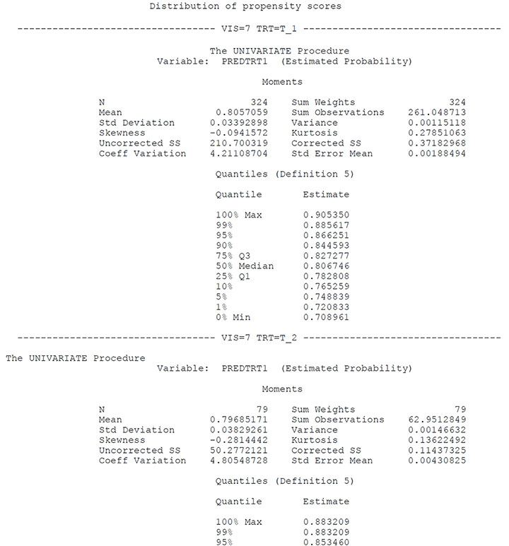
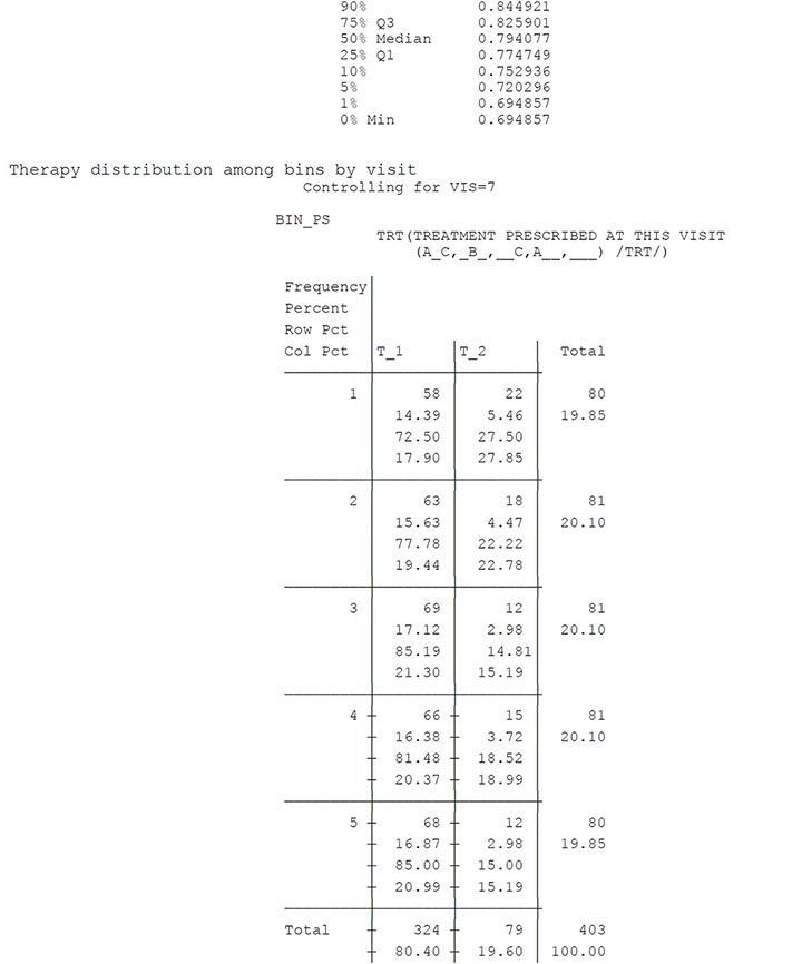
Table 11.2 Summary of Covariate Balance before and after Propensity Score Strata Adjustment (Visit 7)
| Before Subclassification | After Subclassification | |||
| Covariate | F-Statistic | P-value | F-Statistic | P-value |
| Age | .09 | .767 | .03 | .871 |
| Baseline GAF | .42 | .517 | .02 | .895 |
| Baseline BPRS | .18 | .669 | .10 | .748 |
| Previous GAF | 1.23 | .268 | .86 | .354 |
| Previous BPRS | 2.58 | .109 | .47 | .492 |
| Chi-SquareStatistics | P-value | Chi-SquareStatistic | P-value | |
| Previous Event | .66 | .416 | .05 | .820 |
| Previous Hosp | .02 | .879 | .04 | .840 |
Analysis Step 3
In Step 3, estimated probabilities of transitioning between the longitudinal propensity score strata are computed. PROC LOGISTIC in the macro EST (see Program 11.3) conducts the initial calculations for the transition probabilities. A proportional odds logistic model is run, with the propensity score bin as the dependent variable (five possible values) and a simple model with the previous visit’s treatment and propensity bins as covariates. Data manipulation of the output data set is required in order to modify the output cumulative values into the transition values necessary for later analysis steps. At the end of this section, we have included data sets with the transition probabilities for visit 5 to visit 6 and from visit 6 to visit 7 (TRPR_V6 and TRPR_V7).
Program 11.3 Estimation of Transition Probabilities
**********************************************************************;
* STEP 3: Estimate transitional probabilities of the longitudinal *;
* propensity score strata. The first part of this section creates *;
* an analysis data set with variables to denote the propensity *;
* score bin and treatment at each visit (data set UPD which is then *;
* merged with visitwise analysis data sets). Summary statistics on *;
* the propensity score bins and treatments over time can be easily *;
* summarized using PROC FREQ. The EST macro runs a proportional *;
* odds logistic regression model to assess the transitional *;
* probabilities for each possible combination of propensity bin *;
* over time. The steps following the macro compute the transition *;
* probabilities from the parameter estimates of the logistic model *;
**********************************************************************;
* Input for macro denotes the visit number *;
%MACRO PM(VN);
DATA F1_&VN;
SET &VN;
BIN PS & VN = BIN_PS;
TRT & VN = TRT;
KEEP PATSC BIN_PS_&VN TRT_&VN;
RUN;
%PM(V5); RUN;
%PM(V6); RUN;
%PM(V7); RUN;
PROC SORT DATA = F1_V5; BY PATSC; RUN;
PROC SORT DATA = F1_V6; BY PATSC; RUN;
PROC SORT DATA = F1_V7; BY PATSC; RUN;
DATA UPD;
MERGE F1_V5 F1_V6 F1_V7;
BY PATSC;
PROC FREQ DATA = UPD;
TABLES BIN_PS_V5*BIN_PS_V6*BIN_PS_V7;
TITLE 'PATTERN OF BINS OVER TIME'; RUN;
PROC FREQ DATA = UPD;
TABLES TRT_V5 TRT_V6 TRT_V7 TRT_V5*TRT_V6*TRT_V7;
TITLE 'PATTERN OF TRTS OVER TIME'; RUN;
PROC SORT DATA = UPD; BY PATSC; RUN;
PROC SORT DATA = V5; BY PATSC; RUN;
PROC SORT DATA = V6; BY PATSC; RUN;
PROC SORT DATA = V7; BY PATSC; RUN;
DATA V5;
MERGE V5 UPD;
BY PATSC;
DATA V6;
MERGE V6 UPD;
BY PATSC;
DATA V7;
MERGE V7 UPD;
BY PATSC;
ODS LISTING CLOSE;
/* Input for macro includes the analysis data set for a specific visit (INDAT), name for the output data set containing the parameter estimates (PARM_EST), list of variables for the CLASS statement (CLASSVARS), and list of variables in the MODEL statement (MODELVARS). Run macro for the 2nd and 3rd time points to assess transitions. */
%MACRO EST(INDAT, PARM_EST, CLASSVARS, MODELVARS);
PROC LOGISTIC DATA = &INDAT OUTEST = &PARM_EST;
CLASS &CLASSVARS;
MODEL BIN_PS = &MODELVARS;
RUN;
%MEND EST;
%EST(V6, PARM_V6, TRT_V5 BIN_PS_V5, TRT_V5 BIN_PS_V5); RUN;
%EST(V7, PARM_V7, TRT_V5 BIN_PS_V5 TRT_V6 BIN_PS_V6, TRT_V5 BIN_PS_V5 TRT_V6
BIN_PS_V6); RUN;
ODS LISTING;
/* Data trpr_v7 uses the parameter estimates output from the EST macro to compute the actual transition probabilities for time period 2 to 3. Arrays are used in order to more efficiently calculate the 250 different transition probabilities (5x5x5x2: 5 propensity bins at each of 3 time points for each of two treatment patterns of interest). */
DATA TRPR_V7;
SET PARM_V7;
IF _TYPE_ = 'PARMS';
* parameters are set to zero automatically in SAS modeling and are
specifically set to zero here for clarity. *;
INTERCEPT_5 = 0;
BIN_PS_V55 = - BIN_PS_V51 - BIN_PS_V52 - BIN_PS_V53 - BIN_PS_V54;
BIN_PS_V65 = - BIN_PS_V61 - BIN_PS_V62 - BIN_PS_V63 - BIN_PS_V64 ;
TRT_V5T_2 = - TRT_V5T_1;
TRT_V6T_2 = - TRT_V6T_1;
X1 = INTERCEPT_1;
X2 = INTERCEPT_2;
X3 = INTERCEPT_3;
X4 = INTERCEPT_4;
X5 = INTERCEPT_5;
Y1= BIN_PS_V51;
Y2= BIN_PS_V52;
Y3= BIN_PS_V53;
Y4= BIN_PS_V54;
Y5= BIN_PS_V55;
Z1= BIN_PS_V61;
Z2= BIN_PS_V62;
Z3= BIN_PS_V63;
Z4= BIN_PS_V64;
Z5= BIN_PS_V65;
W1= TRT_v5T_1;
W2= TRT_v5T_2;
V1= TRT_v6T_1;
V2= TRT_v6T_2;
run;
DATA TRPR_V7;
SET TRPR_V7;
ARRAY X[5] X1 - X5;
ARRAY Y[5] Y1 - Y5;
ARRAY Z[5] Z1 - Z5;
ARRAY W[2] W1 - W2;
ARRAY V[2] V1 - V2;
ARRAY PRE[5, 5, 5, 2 ];
DO A = 1 TO 2; * LOOP FOR 2 TREATMENT GROUPS *;
DO I = 1 TO 5; * LOOP FOR BINS AT TIME PERIOD 3 *;
DO J = 1 TO 5; * LOOP FOR BINS AT TIME PERIOD 1 *;
DO K = 1 TO 5; * LOOP FOR BINS AT TIME PERIOD 2 *;
* Computation of probabilities using logistic model. Initial (pre)
probabilites are cumulative as they are from proportional odds
model - and are adjusted to individual outcome probabilities here*;
PRE[I, J, K, A ]= EXP(X[I] + W[A] + V[A] + Y[J] + Z[K]) / (1 +
EXP(X[I] + W[A] + V[A] + Y[J] + Z[K]));
TRPR7 = PRE[I, J, K, A ];
IF 2 LE I LE 4 THEN DO;
TRPR7 = PRE[I, J, K, A ] - (EXP(X[I-1] + W[A] + V[A] + Y[J] +
Z[K]) / (1 + EXP(X[I-1] + W[A] + V[A] + Y[J] +
Z[K])));
END;
IF I = 5 THEN DO;
TRPR7 = 1 - (EXP(X[I-1] + W[A] + V[A] + Y[J] + Z[K]) / (1 +
EXP(X[I-1] + W[A] + V[A] + Y[J] + Z[K])));
END;
OUTPUT;
END;
END;
END;
END;;
KEEP A I J K TRPR7;
* Repeat the same process for trpr_v6 as for trpr_v7. Here there are 50 transitional probabilities to compute. *;
DATA TRPR_V6;
SET PARM_V6;
IF _TYPE_ = 'PARMS';
INTERCEPT_5 = 0;
BIN_PS_V55 = - BIN_PS_V51 - BIN_PS_V52 - BIN_PS_V53 - BIN_PS_V54;
TRT_V5T_2 = - TRT_V5T_1;
X1 = INTERCEPT_1;
X2 = INTERCEPT_2;
X3 = INTERCEPT_3;
X4 = INTERCEPT_4;
X5 = INTERCEPT_5;
y1= BIN_PS_V51;
y2= BIN_PS_V52;
y3= BIN_PS_V53;
y4= BIN_PS_V54;
y5= BIN_PS_V55;
z1= TRT_V5T_1;
z2= TRT_V5T_2;
run;
DATA TRPR_V6;
SET TRPR_V6;
ARRAY X[5] X1 - X5;
ARRAY Y[5] Y1 - Y5;
ARRAY Z[2] Z1 - Z2;
ARRAY PRE[5, 5, 3 ]; /* it is a three-dimensional array */
DO A = 1 TO 2;
DO K = 1 TO 5;
DO J= 1 TO 5;
PRE[K, J, A]= EXP(X[K] + Y[J] + Z[A]) / (1 + EXP(X[K] + Y[J] +
Z[A]));
TRPR6 = PRE[K, J, A];
IF 2 LE k LE 4 THEN DO;
TRPR6 = PRE[K, J, A] - (EXP(X[K-1] + Y[J] + Z[A]) / (1 +
EXP(X[K-1] + Y[J] + Z[A])));
END;
IF K = 5 THEN DO;
TRPR6 = 1 - (EXP(X[K-1] + Y[J] + Z[A]) / (1 + EXP(X[K-1] +
Y[J] + Z[A])));
END;
OUTPUT;
END;
END;
END;
KEEP A J K TRPR6 SECTION6; RUN;
Analysis Step 4
In this step, we estimate the expected outcomes for the longitudinal treatment patterns of interest. Specifically, we are interested in the expected outcomes for treatment 1 at all time periods and treatment 2 at all time points. PROC GENMOD (with the NORMAL distribution for our continuous outcome measure) was used to estimate the expected values. The model, with the change in outcome measure at endpoint as the dependent measure, included the previous treatments and previous propensity score strata as dependent measures. The final result of this step is an analysis data set containing the predicted values for each treatment and propensity bin combination over time (2*5*5*5 = 250 combinations: two treatment patterns of interest and 125 propensity bin combinations) —along with the probabilities of those transitions from Step 3. An example listing of this data set (ALL) is provided after Program 11.4.
The listing shows that a patient on treatment 1 at time point 1 in propensity strata 1 had a 56% chance of being in strata 1 at time 2. Furthermore, a patient in strata 1 at time 2 had a 69% chance of remaining in strata 1 at time 3. The expected outcome of a patient on treatment 1 at each time point and in propensity strata 1 at each time point was -8.6.
Program 11.4 Estimation of Expected Outcomes for each Transition Path
**********************************************************************;
* STEP 4: Estimate longitudinal treatment expected outcomes in *;
* groups of interest (AAA and BBB). This code runs a simple model *;
* with only the treatment and propensity score bins at each time- *;
* point included as covariates and the outcome measure as the *;
* dependent variable. This macro can be used to assess sensitivity*;
* via comparisons with other models. After the macro call, the *;
* parameter estimates are output to a data set to allow for *;
* calculation of the expected outcome for all possible transition *;
* paths (all treatment and propensity bin options over time). *;
**********************************************************************;
DATA V7;
SET V7;
TRT_V5_ = TRT_V5;
TRT_V6_ = TRT_V6;
TRT_V7_ = TRT_V7;
DATA OUTCV7;
SET RANKPS;
IF VIS = 7;
KEEP PATSC BAVAR AVAR CAVAR;
PROC SORT DATA = V7; BY PATSC; RUN;
PROC SORT DATA = OUTCV7; BY PATSC; RUN;
DATA ADAT7;
MERGE V7 (IN=A) OUTCV7 (IN=B);
BY PATSC;
IF A AND B;
* Summary statistics on analysis data set *;
PROC MEANS DATA = ADAT7;
CLASS TRT_V5_ TRT_V6_ TRT_V7_;
VAR CAVAR;
TITLE2 'SUMMARY STATS FROM ADAT7'; run;
PROC TABULATE DATA = ADAT7;
CLASS TRT_V5_ TRT_V6_ TRT_V7_;
VAR BAVAR CAVAR;
TABLES (TRT_V5_*TRT_V6_*TRT_V7_)*(N MEAN STD),(BAVAR CAVAR);
TITLE2 'SUMMARY STATS FROM ADAT7'; run;
/* Input for macro includes the analysis data set for a specific visit (DATA_2), name for the output data set containing the parameter estimates (DATA_1), list of variables for the CLASS statement (CLASSVAR2), and list of variables in the MODEL statement (MODELVAR2). */
%MACRO G_ESTS(DATA_2, DATA_1, CLASSVAR2, MODELVAR2);
ODS OUTPUT ParameterEstimates= &data_1 ;
PROC GENMOD DATA = &DATA_2;
CLASS &CLASSVAR2;
MODEL CAVAR = &MODELVAR2 / DIST = NOR LINK = ID;
run;
%MEND G_ESTS;
%g_ests(ADAT7, vis7_OUTCESTS, TRT_V5_ TRT_V6_ TRT_V7_ BIN_PS_V5
BIN_PS_V6 BIN_PS_V7, TRT_V5_ TRT_V6_ TRT_V7_ BIN_PS_V5 BIN_PS_V6
BIN_PS_V7);
run;
* get parameter estimates from model to allow computation *;
* of expected values for all transition paths *;
DATA VIS7_OUTCESTS;
SET VIS7_OUTCESTS;
KEEP PARAMETER LEVEL1 ESTIMATE;
PROC TRANSPOSE DATA = VIS7_OUTCESTS OUT=TR_OUTCESTS;
RUN;
DATA TR_OUTCESTS;
SET TR_OUTCESTS;
INTERCEPT = COL1;
X1 = COL2; * TRT AT V5 *;
X2 = COL3;
Y1 = COL4; * TRT AT V6 *;
Y2 = COL5;
Z1 = COL6; * TRT AT V7 *;
Z2 = COL7;
B1=COL8; B2=COL9; B3=COL10; B4=COL11; B5=COL12; * BIN AT V5 *;
C1=COL13; C2=COL14; C3=COL15; C4=COL16; C5=COL17; * BIN AT V6 *;
L1=COL18; L2=COL19; L3=COL20; L4=COL21; L5=COL22; * BIN AT V7 *;
run;
DATA OUTC;
SET TR_OUTCESTS;
ARRAY X[2] X1 - X2;
ARRAY Y[2] Y1 - Y2;
ARRAY Z[2] Z1 - Z2;
ARRAY B[5] B1 - B5;
ARRAY C[5] C1 - C5;
ARRAY L[5] L1 - L5;
ARRAY PRE[2, 5, 5, 5 ];
DO A = 1 TO 2;
DO J = 1 TO 5;
DO K = 1 TO 5;
DO I = 1 TO 5;
PRE[A, J, K, I ]= COL1 + X[A] + Y[A] + Z[A] + B[J] + C[K] + L[i];
EOUT = PRE[A, J, K, I ];
OUTPUT;
END;
END;
END;
END;
run;
DATA OUTC;
SET OUTC;
KEEP A J K I EOUT;
run;
PROC SORT DATA = TRPR_V7; BY A J K I; RUN;
PROC SORT DATA = OUTC; BY A J K I; RUN;
PROC SORT DATA = TRPR_V6; BY A J K; RUN;
DATA ALL1;
MERGE TRPR_V7 OUTC;
BY A J K I;
DATA ALL;
MERGE ALL1 TRPR_V6;
BY A J K;
SUM_EO = EOUT*(.2)*TRPR6*TRPR7;
IF A = 1 THEN TRTPTTRN = 'AAA';
IF A = 2 THEN TRTPTTRN = 'BBB';
PROC PRINT DATA = ALL;
VAR TRTPTTRN J K I TRPR6 TRPR7 EOUT;
TITLE 'LISTING OF DATASET ALL (TRANSITION PROBS AND EXPECTED OUTCOMES)';
RUN;
Output from Program 11.4
LISTING OF DATASET ALL (TRANSITION PROBS AND EXPECTED OUTCOMES
| Obs | TRTPTTRN | J | K | I | TRPR6 | TRPR7 | EOUT |
| 1 | AAA | 1 | 1 | 1 | 0.56184 | 0.68756 | -8.5755 |
| 2 | AAA | 1 | 1 | 2 | 0.56184 | 0.23807 | -10.9945 |
| 3 | AAA | 1 | 1 | 3 | 0.56184 | 0.05502 | -13.0868 |
| 4 | AAA | 1 | 1 | 4 | 0.56184 | 0.01634 | -17.8012 |
| 5 | AAA | 1 | 1 | 5 | 0.56184 | 0.00301 | -20.6457 |
| 6 | AAA | 1 | 2 | 1 | 0.28214 | 0.48647 | -11.0129 |
| 7 | AAA | 1 | 2 | 2 | 0.28214 | 0.35624 | -13.4318 |
| 8 | AAA | 1 | 2 | 3 | 0.28214 | 0.11345 | -15.5242 |
| 9 | AAA | 1 | 2 | 4 | 0.28214 | 0.03687 | -20.2385 |
| 10 | AAA | 1 | 2 | 5 | 0.28214 | 0.00697 | -23.0830 |
| 11 | AAA | 1 | 3 | 1 | 0.11399 | 0.22977 | -12.3396 |
| 12 | AAA | 1 | 3 | 2 | 0.11399 | 0.39809 | -14.7585 |
| 13 | AAA | 1 | 3 | 3 | 0.11399 | 0.24504 | -16.8509 |
| 14 | AAA | 1 | 3 | 4 | 0.11399 | 0.10530 | -21.5652 |
| 15 | AAA | 1 | 3 | 5 | 0.11399 | 0.02180 | -24.4097 |
| . . . . | |||||||
| 125 | AAA | 5 | 5 | 5 | 0.62377 | 0.75457 | -17.1169 |
| . . . . | |||||||
Analysis Step 5
This step utilizes the output of Steps 3 and 4 (contained in data set ALL) to estimate the average of the potential outcomes for the longitudinal treatment patterns of interest (treatment 1 at all time points [denoted AAA] and treatment 2 at all time points [denoted BBB]). This is accomplished using simple summations of the appropriate probabilities in data set ALL. The summation produces an estimated treatment difference favoring treatment 1 of 2.5 points on the BPRS scale (see Output from Program 11.5).
Program 11.5 Estimation of Outcomes in Treatment Patterns of Interest
**********************************************************************;
* STEP 5: Estimate the average, over all patients, of the potential *;
* outcomes for longitudinal treatment groups of interest (AAA vs *;
* BBB). This code uses the expected values for all patterns *;
* created in step 4 and sums the values across the corresponding *;
* patterns of interest. The final estimates are then printed. *;
**********************************************************************;
PROC SORT DATA = ALL;
BY A; RUN;
DATA ALL;
SET ALL;
IF A = 1 THEN DO; * COUNTERS FOR TREATMENT 1 *;
WTEST_AAA + SUM_EO;
SUM_TRPR6A + TRPR6;
SUM_TRPR7A + TRPR7;
END;
IF A = 2 THEN DO; * COUNTERS FOR TREATMENT 2 *;
WTEST_BBB + SUM_EO;
SUM_TRPR6B + TRPR6;
SUM_TRPR7B + TRPR7;
END;
DUM = 1;
PROC SORT DATA = ALL;
BY DUM; RUN;
DATA ALL;
SET ALL;
BY DUM;
IF LAST.DUM;
DIFF = WTEST_AAA - WTEST_BBB;
KEEP WTEST_AAA WTEST_BBB DIFF;
PROC PRINT DATA = ALL;
TITLE 'FINAL ESTIMATE DATASET';
TITLE2 'WTEST_AAA: ESTIMATED RESPONSE FOR LONGITUDINAL TREATMENT PATTERN AAA';
TITLE3 'WTEST_BBB: ESTIMATED RESPONSE FOR LONGITUDINAL TREATMENT PATTERN BBB';
TITLE4 'DIFF: ESTIMATED DIFFERENCE IN RESPONSE BETWEEN TWO TREATMENT PATTERNS';
RUN;
Output from Program 11.5
FINAL ESTIMATE DATASET
WTEST_AAA: ESTIMATED RESPONSE FOR LONGITUDINAL TREATMENT PATTERN AAA
WTEST_BBB: ESTIMATED RESPONSE FOR LONGITUDINAL TREATMENT PATTERN BBB
DIFF: ESTIMATED DIFFERENCE IN RESPONSE BETWEEN TWO TREATMENT PATTERNS
| Obs | WTEST_ AAA |
WTEST_ BBB |
DIFF |
| 1 | -13.0024 | -10.1465 | -2.85589 |
Analysis Step 6
In this step, Steps 3 through 5 are repeated using a bootstrap algorithm (5,000 replications used here) in order to estimate the variability of our propensity score sub-classification treatment difference estimate. The specific code is not shown, but simply creates a loop to repeat the process 5,000 times and output the resulting treatment difference estimate. The distribution of treatment difference estimates is summarized by PROC UNIVARIATE. Using the percentile method, the 95% 2-sided confidence interval was found to be (-6.91, 1.30) with a corresponding p-value of 0.185.
Output from Analysis Step 6
SUMMARY STATS ON BOOTSTRAP DIFFERENCES: AAA - BBB
The UNIVARIATE Procedure
Variable: DIFF
Moments
| N | 5000 | Sum Weights | 5000 |
| Mean | -2.7978146 | Sum Observations | -13989.073 |
| Std Deviation | 2.09761783 | Variance | 4.40000058 |
| Skewness | 0.02795663 | Kurtosis | -0.1326878 |
| Uncorrected SS | 61134.4344 | Corrected SS | 21995.6029 |
| Coeff Variation | -74.973441 | Std Error Mean | 0.0296648 |
Basic Statistical Measures
| Location | Variability | ||
| Mean | -2.79781 | Std Deviation | 2.09762 |
| Median | -2.79368 | Variance | 4.40000 |
| Mode | . | Range | 14.18360 |
| Interquartile Range | 2.87671 | ||
Tests for Location: Mu0=0
| Test | -Statistic- | ---- p Value---- | ||
| Student's t | t | -94.3143 | Pr > |t| | <.0001 |
| Sign | M | -2028 | Pr >= |M| | <.0001 |
| Signed Rank | S | -5878113 | Pr >= |S| | <.0001 |
Quantiles (Definition 5)
| Quantile | Estimate |
| 100% Max | 4.8827501 |
| 99% | 1.9440237 |
| 95% | 0.6811120 |
| 90% | -0.0688069 |
| 75% Q3 | -1.3916694 |
| 50% Median | -2.7936758 |
| 25% Q1 | -4.2683819 |
| 10% | -5.4915107 |
| 5% | -6.2668682 |
| 1% | -7.6076745 |
| 0% Min | -9.3008516 |
Frequency Counts
Percents
Value Count Cell Cum
| . . . | |||
| -6.908590145030 | 1 | 0.0 | 2.5 |
| . . . | |||
| 1.295190177818 | 1 | 0.0 | 97.5 |
Sensitivity / Model Checks
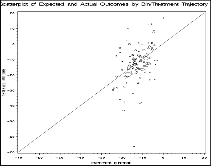
As mentioned previously, a key feature of using regression on the longitudinal propensity score is that we can more easily check the relative validity of the models. Here we present SAS code (Program 11.6) to graphically depict the predictive accuracy of the outcome model. The code produces a scatterplot of the predicted and actual means for each bin and treatment combination—with the area of each plotted circle representing the sample size in each longitudinal subclass. From the output, there are noted outliers, though all subclasses of reasonable sample sizes were well predicted by the model.
To further assess the validity of the models, we also followed the two approaches presented in Section 11.2. First, we assessed model improvement for both the transition and outcome models using the AIC criteria. Second, we re-ran the outcome model using only the subset of patients who did not switch treatments during the study. The AIC criteria can be assessed by modifying the MODEL (transition and outcome) statements in the EST (Program 11.3) and G_ESTS (Program 11.4) macros (not shown). For these data, the AIC was slightly improved by the inclusion of the treatment interactions (for example, visit 5 by visit 6 and visit 6 by visit 7 interactions) and the treatment by propensity bin interactions (for example, visit 5 treatment by visit 5 bin). However, the inferences from this model were the same and the model was less stable—with a much larger variance from the bootstrap evaluation. Thus, the simple model results are retained here. The same SAS code was also used to assess the outcome using the subset of patients not switching treatments during the study. This was accomplished by modifying the data set entering the analysis macros. Once again, inferences from this approach were similar.
Program 11.6 Graphical Assessment of Analysis Models
********************************************************;
** Graph of observed and expected outcomes to assist **;
** in model assessment **;
********************************************************;
PROC MEANS DATA = ADAT7 NOPRINT;
CLASS TRT_V5_ TRT_V6_ TRT_V7_ BIN_PS_V5 BIN_PS_V6 BIN_PS_V7;
VAR CAVAR;
OUTPUT OUT = MEANOUT N = NPT MEAN = AVGVAL; RUN;
DATA OUTC;
SET OUTC;
BIN_PS_V5 = J;
BIN_PS_V6 = K;
BIN_PS_V7 = I;
DATA MEANOUT;
SET MEANOUT;
IF (TRT_V5_ = 'T_1' AND TRT_V6_ = 'T_1' AND TRT_V7_ ='T_1' AND
BIN_PS_V5 NE . AND BIN_PS_V6 NE . AND BIN_PS_V7 NE .) OR
(TRT_V5_ = 'T_2' AND TRT_V6_ = 'T_2' AND TRT_V7_ ='T_2' AND
BIN_PS_V5 NE . AND BIN_PS_V6 NE . AND BIN_PS_V7 NE .);
IF TRT_V5_ = 'T_1' AND TRT_V6_ = 'T_1' AND TRT_V7_ ='T_1’ THEN A = 1;
IF TRT_V5_ = 'T_2' AND TRT_V6_ = 'T_2' AND TRT_V7_ ='T_2' THEN A = 2;
PROC SORT DATA = OUTC; BY A BIN_PS_V5 BIN_PS_V6 BIN_PS_V7; RUN;
PROC SORT DATA = MEANOUT; BY A BIN_PS_V5 BIN_PS_V6 BIN_PS_V7; RUN;
DATA GRPH;
MERGE OUTC (IN=X) MEANOUT (IN=Y);
BY A BIN_PS_V5 BIN_PS_V6 BIN_PS_V7;
IF X AND Y;
TITLE 'Scatterplot of Expected and Actual Outcomes by Bin/Treatment Trajectory';
SYMBOL1 C=RED V=CIRCLE;
AXIS1 LABEL = (ANGLE=90 "OBSERVED OUTCOME") ORDER = (-70 TO 20 BY 10);
AXIS2 LABEL = (ANGLE=0 "EXPECTED OUTCOME") ORDER = (-70 TO 20 BY 10);
PROC GPLOT DATA=GRPH;
BUBBLE AVGVAL*EOUT = NPT / vaxis = axis1 haxis = axis2;
PLOT AVGVAL*EOUT = 1 / vaxis = axis1 haxis = axis2;
RUN;
Output from Program 11.6
The method presented in this chapter can be viewed first as an extension of the propensity score regression adjustment methods to a longitudinal setting. It can also be seen as a robust, yet easier, way of applying and extending g-computation-based methods by replacing the full covariate history with the longitudinal propensity scores. In the chapter, we gave a quick and practical overview of the methodology and presented a detailed illustration of the steps needed to evaluate longitudinal treatment using regression models on the propensity scores.
Achy-Brou, A. C., C. E. Frangakis, and M. Griswold. “Estimating treatment effects of longitudinal designs using regression models on propensity scores.” Biometrics. Published online October 10, 2009. DOI: 10.1111/j.1541-0420.2009.01334.x.
Austin, P. C. 2008. “Goodness-of-fit diagnostics for the propensity score model when estimating treatment effects using covariate adjustment with the propensity score.” Pharmacoepidemiology and Drug Safety 17(12): 1202–1217.
Horvitz, D. G., and D. J. Thompson. 1952. “A generalization of sampling without replacement from a finite universe.” Journal of the American Statistical Association 47: 663 685.
Neyman, J. 1928. “On the application of probability theory to agricultural experiments. Essay on principles.” Section 9, translated. 1990. Statistical Science 5: 465–80.
Robins, J. M. 1987. “A graphical approach to the identification and estimation of causal parameters in mortality studies with sustained exposure periods.” Journal of Chronic Diseases 40, Supplement 2: 139S–161S.
Robins, J. M., M. A. Hernán, and B. Brumback. 2000. “Marginal structural models and causal inference in epidemiology.” Epidemiology 11: 550–560.
Rosenbaum, P. R, and D. B. Rubin. 1983. “The central role of the propensity score in observational studies for causal effects.” Biometrika 70: 41–55.
Rosenbaum, P. R., and D. B. Rubin. 1984. “Reducing bias in observational studies using subclassification on the propensity score.” Journal of the American Statistical Association 79: 516–24.
Rubin, D. B. 1974. “Estimating causal effects of treatments in randomized and nonrandomized studies.” Journal of Educational Psychology 66(5): 688–701.
Rubin, D. B. 1978. “Bayesian inference for causal effects: the role of randomization.” Annals of Statistics 6: 34–58.
Segal, J. B., M. Griswold, A. C. Achy-Brou, and R. Herbert. 2007. “Using propensity scores subclassification to estimate effects of longitudinal treatments: an example using a new diabetes medication.” Medical Care 45: S149–157.
Tsiatis, A. A. 2006. Semiparametric Theory and Missing Data (page 336). New York: Springer-Verlag.&Tunis, S. L., D. E. Faries, A. W. Nyhuis, B. J. Kinon, H. Ascher-Svanum, and R. Aquila. 2006. “Cost-effectiveness of olanzapine as first-line treatment for schizophrenia: results from a randomized, open-label, 1-year trial. Value in Health 9(2): 77–89.