
Costs and Cost-Effectiveness Analysis Using Propensity Score Bin Bootstrapping
14.2 Propensity Score Bin Bootstrapping
14.3 Example: Schizophrenia Effectiveness Study
Analysis of cost and cost-effectiveness data is of increasing importance among health care decision-makers in today’s economic climate. Propensity score bin bootstrapping is a new analytical approach that addresses three fundamental challenges of observational cost data analysis:
1. the typical skewness of cost distributions
2. the need to estimate mean rather than median or other robust measures
3. the need to adjust for selection bias
In this chapter, an overview of various methodologies for analyzing cost data is presented along with SAS code to perform a propensity score bin bootstrapping analysis comparing the mean cost and cost-effectiveness of competing interventions.
14.1.1 Overview
As the cost of health care in the United States continues to grow, cost and cost-effectiveness analyses have become key factors in medical decision-making. For instance, health care payers have great interest in analyses such as comparing the total costs of care from two or more competing treatment regimens. However, the appropriate analysis for comparing cost data between groups can be complex because it must address the potential skewness in the data, estimate mean costs, and adjust for important baseline treatment group differences.
Cost data from medical studies are typically skewed because a subset of patients may have very high costs due to resource-intensive treatments (such as hospitalizations), while another subset may perform very well and utilize few or less costly medical resources. Second, medians or trimmed means are commonly used statistical measures of central tendency for describing populations with outliers. Unfortunately, these measures are unrealistic and misleading for payers responsible for all of the costs incurred by a patient population. Mean costs are more relevant here; the population size times the median cost is not representative of the total liability to the payer (Ramsey et al., 2005; Doshi et al., 2006). Third, the most realistic (generalizable) cost data typically come from naturalistic research. Randomized, clinical trials use protocols with regularly scheduled health care provider visits (often more frequent than actual practice), free access to many resources, structured dosing, strict entry criteria, and mandated compliance. All of these issues clearly limit the generalizability of the clinical trial cost estimates (Grimes and Schulz, 2002; Revicki and Frank, 1999; Roy-Byrne et al., 2003). On the other hand, naturalistic studies lacking randomization to treatment are subject to treatment selection bias on baseline patient characteristics that needs to be accounted for in analyses (Rosenbaum and Rubin, 1983).
Several approaches to the analyses of cost data appear in the published literature (Doshi et al., 2006):
• t-tests/ANOVA
• rank-based nonparametric tests
• transformation approaches
• generalized linear models
• bootstrapping
In this chapter, we review published guidance on analysis and reporting of economic data, briefly review commonly used methodology, introduce and discuss a new approach—propensity score bin bootstrapping (PSBB)—and demonstrate an analysis of cost data from a schizophrenia trial using SAS software. Given the availability of multiple approaches and the fact that the validity of each is based on different assumptions, it is critical that researchers understand and evaluate the assumptions behind cost analyses, perform appropriate sensitivity analyses, and provide transparency in presenting their work. This will allow consumers to fully assess the robustness of the findings and appropriately utilize the information in decision-making.
Last, medical payer decision-makers are often faced with a tradeoff—that is, a new medication may have some advantage over a competing medication, but that advantage comes at a higher financial cost. Cost-effectiveness analyses, where one estimates the incremental cost necessary to gain some unit of benefit (for example, quality-of-life years) by using the more expensive treatment options, typically involve the assessment of either an incremental cost-effectiveness ratio (ICER) or an incremental net benefit (INB) (Willan and Briggs, 2006). Because the INB approach is demonstrated in the following chapter, we will demonstrate the ICER approach here.
14.1.2 Economic Analysis Guidelines
Over the past years, many guidelines have been published on the study design, data collection, data analysis, and reporting of economic analyses (Bouckaert and Crott, 1997; Ramsey et al., 2005; Rutten-van MÖlken et al., 1994). Recently, the International Society of Pharmacoeconomics and Outcomes Research (ISPOR) commissioned several task forces to provide guidance on topics related to economic analyses. For instance, Drummond and colleagues (2003) provided a review of 15 previous guidelines for reporting economic analyses. The previous guidelines were consistent on topics such as cost/resource measurement, discounting, target audience, and perspective of the analyses. However, Drummond and colleagues cited a need for additional guidance on multiple topics, including transparency of reporting, extensive use of assumptions, and extrapolations. Subsequently, a task force was chartered to create updated guidance based on consensus of good practices for the design, conduct, analysis, and reporting of economic studies alongside clinical trials (Ramsey et al., 2005). Garrison and colleagues (2007) have also recently provided guidance for the use of real-world data for coverage and payment decisions. For checklists and more detailed discussion of these issues, refer to these references.
Regarding specific statistical approaches, detailed information is typically not provided in such guidance documents. However, Rutten-van MÖlken and colleagues (1994) stressed the need to perform Duan “smearing” to eliminate downwards bias in mean cost estimates resulting from retransforming log cost estimates. The ISPOR guidelines stress the importance of assessing uncertainty, performing sensitivity analyses, and addressing missing data (Ramsey et al., 2005). In addition, they emphasize the need to assess mean costs—and mention bootstrapping as a robust analytical approach. The general issue of the need to assess uncertainty in estimates is a common basic theme across all guidance documents.
14.1.3 Current Methodology Overview
Despite the existence of such guidelines, a recent survey of analytical methods used for cost analyses in the literature revealed a lack of consistent application of quality methods. Doshi and colleagues (2006) evaluated statistical methods utilized for economic analyses for 115 manuscripts reported in the MEDLINE database in 2003. They concluded that the quality of statistical methods used in economic evaluations was poor in the majority of studies. For instance, over 40% failed to report an estimate of uncertainty in their results, and less than 25% of the studies making statistical comparisons utilized nonparametric estimates of mean costs (for example, nonparametric bootstrapping). The most commonly used statistical approach for comparing costs between groups per Doshi (2006) was the simple t-test. The t-test does assess the differences in mean costs and, with the use of ANCOVA, can adjust for linear effects of covariates. However, the distribution of costs in the majority of cases is highly skewed and non-normal. Thus, the validity of the test relies on the central limit theorem and the estimates of the means. The test can be adversely affected by outliers. There are no clear guidelines on when the sample size is large enough relative to the observed level of skewness for a t-test to be appropriate, though one simulation study has suggested 500 per group is sufficient (Lumley et al., 2002). Thus, while the use of such tests may be appropriate in a given setting, sensitivity analyses are clearly warranted.
Rank tests, such as the Wilcoxon-ranked sum test, are nonparametric and simple to perform using SAS (with PROC NPAR1WAY). However, these approaches assess location differences, which, in general, are not differences in mean costs unless the unrealistic assumption of symmetry is met (in which case the median and mean coincide). Medians and other robust estimators are useful for describing the distribution of costs; however, such approaches are not relevant for statistical cost comparisons.
A common simple approach for comparing group costs is to transform the data to address the skewness and normalize the data using a log, square root, or other transformation. Standard, normal statistical methods such as t-tests and ANOVA can then be utilized to compare the groups. Such an approach is easily implemented using SAS functions (for example, the LOG function) and PROC GLM or PROC MIXED. However, a transformation approach can result in misleading results unless key assumptions are satisfied. One obvious assumption is that the transformation produces normality (or at least relies on the central limit theorem). While perhaps less obvious, what is actually more important is that standard test statistics assume that variances of the transformed costs for each treatment group are equal.
To illustrate the basic difficulty, suppose that treatment H with a high acquisition cost is compared, on a cost basis, with treatment L with a low acquisition cost. The low cost (left-hand) tail of the distribution of total accumulated cost over any fixed period of time will then be dominated by patients treated with L. The only way that H could effectively compete on cost with L would be for H to reduce, relative to L, the likelihood of high accumulated costs. In other words, the high cost (right-hand) tail of the distribution of total accumulated cost would then also be dominated by patients treated with L. To be remotely competitive on mean cost, treatment H must (greatly) reduce the variability in accumulated costs. Obviously, if a cost analyst fails to examine these distributions and perhaps unknowingly assumes that variances are equal, treatment H has been unfairly placed at a great disadvantage.
When variances are not equal, comparison of transformed means, which are functions of both the means and the variances on the initial cost scale, can yield badly biased results. This helps explain retransformation problems that have been discussed extensively in the literature (Duan, 1983; Manning, 1998; Mullahy, 1998; Gianfrancesco et al., 2002).
Generalized linear models—which can be fitted using PROC GENMOD—are an additional approach to assessing cost data. Within PROC GENMOD, one can specify a link function and distribution directly, avoiding these retransformation issues. This method obviously requires a distributional assumption, but it allows for easy adjustment of covariates. The SAS/STAT User’s Guide (1999; Example 29.3) provides example code for an analysis of data assuming a gamma distribution using PROC GENMOD that could be applied to cost data. Refer to Lindsey and Jones (1998) for details about choosing between various generalized linear models.
Nonparametric bootstrapping is a technique where an empirical distribution of the test statistic (for example, the mean cost difference between groups) is constructed through resampling with replacement from the observed data. Though computationally intensive, bootstrapping is an attractive alternative for analysis of cost data because it is a nonparametric approach that can directly address arithmetic means. Inferences can be drawn from the empirical distribution using confidence intervals (CIs) formed by the percentile method, bias corrected method, bias corrected and accelerated method, or the percentile–t method (Briggs et al., 1997; DiCiccio and Efron, 1996). While more detailed arguments are possible (Chernick, 1999), a general recommendation is that 5,000 to 10,000 replications be utilized when forming confidence intervals. The validity of the bootstrap approach does rely on asymptotic assumptions—because the observed data must adequately represent the population distribution. While there is no clear guidance on what sample size is sufficient, Chernick provides a general rule of thumb (n>50) and states that sample size considerations should not be altered when using bootstrapping compared with other approaches. While the bootstrap approach allows for estimation of means without making assumptions about the shape of the distribution, by itself it does not allow for adjustment for the confounding variables necessary for addressing group differences. However, this shortcoming can be addressed by incorporating propensity score stratification, as described in the next section.
Combined assessments of both cost and effectiveness typically utilize either an ICER or an INB approach. In this chapter, we consider the use of the ICER approach. The ICER is simply the ratio of the treatment group difference in cost divided by the treatment group difference in effectiveness. Added statistical complexity comes when measures of uncertainty in the ICER point estimate are needed to draw inferences. Several different approaches have been utilized, including a Taylor Series method, Fieller Theorem method, and bootstrapping (Obenchain et al., 1997; Polsky et al., 1997; Willan and Briggs, 2006). For consistency, we focus on the bootstrap approach for determining degrees of dominance using observed incremental cost-effectiveness quadrant confidence levels (Obenchain et al., 2005). When using bootstrapping, one can assess uncertainty in the cost difference, the effectiveness difference, and the cost-effectiveness ratio simultaneously. For each bootstrap sample, one retains both the cost difference and the effectiveness difference from the selected patients—thus retaining any implied correlation structure between cost and effectiveness in the actual data.
14.2 Propensity Score Bin Bootstrapping
The PSBB approach is a potentially useful tool for cost-related analyses because it addresses arithmetic means, adjusts for confounding factors, and does not make distributional assumptions (Obenchain, 2003-2006). The first step in a PSBB analysis is to compute the propensity score for each patient using logistic regression and then group the propensity scores into five strata of equal size determined by estimated propensity score quintiles (Rosenbaum and Rubin, 1984). A thorough assessment should then be made to verify that one’s propensity score estimates produce balanced covariate distributions between treatments within each stratum and that there is sufficient overlap of propensity score estimates between the treatment groups. Because the details of assessing the quality of a propensity model are covered in Chapters 2 through 4, they are not repeated here.
Second, within each treatment group, bootstrap resamples of fixed size are drawn within each stratum—with the total number of samples equaling the total number of patients. For instance, if N = 100 for treatment 1 and N = 200 for treatment 2, then 20 bootstrap samples of treatment 1 patients are taken from each strata, and 40 bootstrap samples of treatment 2 patients are taken from each of the five strata (regardless of the actual number of patients in each strata for each treatment group). For analyses comparing costs, the difference in mean total costs between treatment groups is computed for each replication, and a large number of replications generates the bootstrap distribution of mean cost differences. The percentile method, which identifies the 2.5% and 97.5% points of the distribution of bootstrap order statistics, is one simple way to generate a 95% two-sided confidence interval of the difference in mean costs. Other alternatives include the bias corrected and accelerated (BCa) method (Briggs et al., 1997; DiCiccio and Efron, 1996).
When assessing cost-effectiveness using PSBB, both the cost measure and the effectiveness measure are retained from each patient selected by the resampling, and the ICER is computed for each bootstrap sample. A display of the uncertainty of the ICER is then provided as a bivariate scatter plot of these differences on the cost-effectiveness plane, as described by Obenchain and colleagues (2005).
14.3 Example: Schizophrenia Effectiveness Study
To illustrate PSBB using SAS, we will analyze simulated cost and effectiveness data based on a 1-year, randomized, open-label, naturalistic study of patients with schizophrenia or schizoaffective disorder who were randomly assigned to initial treatment with one of three treatment regimens as reported by Tunis and colleagues (2006). The study was naturalistic in the sense that after randomization patients were treated as in a usual treatment setting and allowed to switch or stop medications and remain in the study. For simplicity, the analysis here focuses on the comparison of total 1-year costs (intent to treat) and cost-effectiveness (with effectiveness defined as estimated days in response [Nyhuis et al., 2003]) between two treatment groups labeled A and B. There were no significant differences in any baseline measure between groups—due to the randomization. However, because most analyses of observational data require adjustment for treatment-selection bias, we illustrate this adjustment using the same covariates examined by Tunis and colleagues (2006). To illustrate distinctions between alternative approaches, we compare the PSBB results to those from the log-transformation and the generalized linear modeling approaches. SAS code for these comparisons is not provided because it is easily accomplished using PROC GLM, PROC MIXED, or PROC GENMOD with PROC PLOT.
Before running the PSBB analysis, we examined the distribution of costs and we present summary statistics for the simulated data (see Program 14.1). The histogram (Output from Program 14.1) shows the high level of skewness and the large variability of the cost data. Summary statistics reveal that treatment A had a slightly lower mean cost and a slightly higher median cost as compared to treatment B.
Program 14.1 Display of Data and Summary Statistics
**************************************************;
** key variables from data set **;
** therapy – randomized treatment group **;
** totcost – total 1-year costs **;
** respdays – estimated responder days(BPRS) **;
** inv – investigational site number **;
** bs_bprsc – baseline bprs level **;
** age – age in years **;
** inpatst – inpatient status at baseline **;
** subsabdx – substance abuse diagnosis **;
** psycdur – duration of psychiatric problems **;
** hospestmo – duration of hosp in past year **;
** insured – insurance status **;
**************************************************;
ods rtf file="D:TempICER_SumCostEff.rtf"
style=minimal;
proc tabulate data = icer;
class therapy;
var respdays totcost;
tables therapy,
(totcost='Total Costs' respdays='Response Days (BPRS)')*
(N*FORMAT=3. P25 MEDIAN P75 MEAN STD);
title 'Summary of costs and effectiveness measures by therapy';
run;
ods rtf close;
proc sort data = ICER;
by therapy; run;
proc univariate data =ICER noprint;
by therapy;
var totcost;
histogram / lognormal(fill l=b) cfill=yellow midpoints =
2500 to 152500 by 5000;
title h=2.5 lspace=1 "Test histogram: raw costs – lognormal
distribution";
run;
data icer2; set icer;
group=floor(totcost/10000);
run;
proc sort data=icer2; by therapy group;
run;
filename MYFILE "D:TempICER_TOTCOST.gif";
goptions reset=all device=gif gsfname=MYFILE gsfmode=replace htext=1
ftext=swiss rotate=landscape;
proc format;
value charge 0='<1';
run;
legend1 label=none across=3 value=(height=1.3) cborder=black cblock=gray;
pattern1 v=solid c=black;
pattern3 v=solid c=LIBRGR ;
pattern2 v=L1 c=black;
footnote1 h=1.5 'Total Costs (10 thou. $)';
title 'Summary of Total Costs by Initial Therapy’;
AXIS1 LABEL=none value=(H=1.5 C=BLACK);
AXIS2 LABEL=(H=2 C=BLACK angle=90 "Frequency" J=CENTER) value=(H=1.5
C=BLACK);
AXIS3 label=none value=none;
PROC GCHART data=ICER2;
format group charge.;
VBAR therapy/patternid=subgroup subgroup=therapy group=group space=0
ref=(10 to 120 by 10) gaxis=axis1 raxis=axis2 maxis=axis3
legend=legend1;
run;
quit;
Output from Program 14.1
Summary of costs and effectiveness measures by therapy
| Total Costs | ||||||
| N | P25 | Median | P75 | Mean | Std | |
| THERAPY | 223 | 4841.09 | 8467.46 | 22796.24 | 20863.59 | 28995.86 |
| A | ||||||
| B | 210 | 2899.83 | 7633.27 | 25269.44 | 21227.37 | 30992.32 |
| Response Days (BPRS) | ||||||
| N | P25 | Median | P75 | Mean | Std | |
| THERAPY | 218 | 20.48 | 97.66 | 229.70 | 129.23 | 117.63 |
| A | ||||||
| B | 200 | 10.38 | 96.63 | 212.06 | 123.74 | 118.29 |

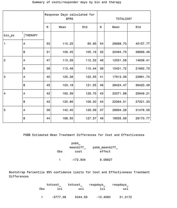
Program 14.2 provides the SAS code for the PSBB analysis. After preliminary calculation of the summary statistics necessary for later computation of confidence intervals, the first main step in the analysis is to compute the propensity score for each patient and form the propensity score strata (using quintiles). This is accomplished using the GENMOD and RANK procedures. Only a brief assessment of the quality of the propensity model is made here—simply utilizing PROC FREQ to confirm adequate numbers of patients per treatment group within each stratum. A lack of patients from either treatment group within a stratum is an indication that there is insufficient overlap (common support) between the two groups to make reliable comparisons (Rosenbaum and Rubin, 1984). Macro PSBB then creates a stratified bootstrap sample of both cost and effectiveness measure values. The inputs to the macro are the number of replications desired, the cost measure, the effectiveness measure, the input data set, and the treatment indicator variable. We used 10,000 bootstrap samples as confidence intervals of interest. The bootstrap distribution for each measure, the confidence intervals for each measure using both the percentile and BCa approaches, the bootstrap distribution of the ICER, and a graphical display of the variability in the ICER are produced.
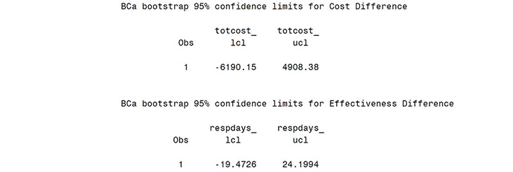
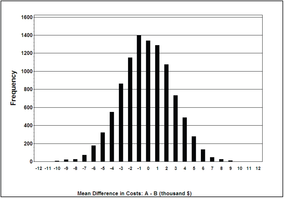
From the Output from Program 14.2 (scatter plot), the bootstrap distribution for total cost difference is centered near zero and shows the large variability in mean costs. The estimated mean treatment difference was $-173 (treatment A-treatment B) and neither the percentile method, 95% CI of (-5777, 5345), nor the bias corrected and accelerated approach, 95% CI of (-6190, 4908), suggests a significant difference in mean costs. Similarly, non-significant differences were observed in the effectiveness measure (9.1 more days of response on treatment A with a 95% CI of -13.4 to +31.3 days).
Program 14.2 SAS Code for Propensity Score Bin Bootstrapping Analysis
TITLE 'PSBB ANALYSIS';
PROC PRINTTO LOG='D:TEMPPSBBLog.log' NEW; RUN;
** Assign summary statistics utilized in analysis code below **;
** Values not computed here to focus code on cost analysis steps **;
%let nc1 = 210; * Sample size for group B with cost data *;
%let nc2 = 223; * Sample size for group A with cost data *;
%let ne1 = 200; * Sample size for group B with effectiveness data *;
%let ne2 = 218; * Sample size for group A with effectiveness data *;
%let mc1 = 21227; * Mean of cost variable for group B *;
%let mc2 = 20864; * Mean of cost variable for group A *;
%let me1 = 123.74; * Mean of effectiveness variable for group B *;
%let me2 = 129.23; * Mean of effectiveness variable for group A *;
** Compute statistic used later in bootstrap CI calculations **;
data icer;
set icer;
* Compute score statistic *;
if therapy = 'A' then do;
mnc1 = (&nc2*&mc2 - totcost) / (&nc2 - 1);
* Mean of group without current obs *;
mne1 = (&ne2*&me2 - respdays) / (&ne2 - 1);
* Mean of group without current obs *;
diffc1 = mnc1 - &mc2;
* Mean diff between groups without current obs *;
diffe1 = mne1 - &me2;
* Mean diff between groups without current obs *;
uc = (&mc2 - &mc1 - diffc1);
ue = (&me2 - &me1 - diffe1);
* Diff between overall and estimate without curren obs *;
end;
if therapy = 'B' then do;
mnc1 = (&nc1*&mc1 - totcost) / (&nc1 - 1);
* Mean of group without current obs *;
mne1 = (&ne1*&me1 - respdays) / (&ne1 - 1);
* Mean of group without current obs *;
diffc1 = &mc1 - mnc1;
* Mean diff between groups without current obs *;
diffe1 = &me1 - mne1;
* Mean diff between groups without current obs *;
uc = (&mc2 - &mc1 - diffc1);
ue = (&me2 - &me1 - diffe1);
* Diff between overall and estimate without current obs *;
end;
if therapy = 'A' then ther = 1;
if therapy = 'B' then ther = 0;
run;
/** Compute acceleration constant for later BCa CI calculations **/
data accel;
set icer;
dm = 1;
uc_cub + uc**3;
ue_cub + ue**3;
uc_sqr + uc**2;
ue_sqr + ue**2;
keep patient dm uc ue uc_cub ue_cub uc_sqr ue_sqr;
run;
proc sort data = accel; by dm;
run;
data accel2;
set accel;
by dm;
if last.dm;
c_aconst = uc_cub / (((uc_sqr**1.5))*6);
e aconst = ue_cub / (((ue_sqr**1.5))*6);
run;
**Assign the c_aconst and e_aconst to macro variables for BCa calculation
in macro PSBB **;
data _null_; set accel2;
call symput('c_aconst', trim(left(c_aconst)));
call symput('e_aconst', trim(left(e_aconst)));
run;
%put c_aconst=&c_aconst e_aconst=&e_aconst;
/*****************************************************
** Compute propensity score strata **
*****************************************************/
option spool;
ods listing close;
proc genmod data = icer;
class inv inptatst subsabdx bs_bprsc insured;
model therapy = inv bs_bprsc age inptatst subsabdx psycdur hospestmo
insured / dist = bin link = logit type3 obstats;
output out=pred6 pred = prdct;
run;
ods listing;
data premab;
set pred6;
predmo = 1-prdct;
predmc = prdct;
keep patient predmo predmc therapy ther totcost respdays age
gender inptatst subsabdx insured hospestmo psycdur bs_bprsc;
run;
proc rank data = premab groups = 5 out = rankmab;
ranks rnkm_ab;
var predmo;
run;
data rankmab;
set rankmab;
bin_ps = rnkm_ab + 1;
run;
proc sort data = rankmab;
by therapy;
run;
proc univariate data = rankmab;
by therapy;
var predmo;
title 'Distribution of propensity scores: oc';
run;
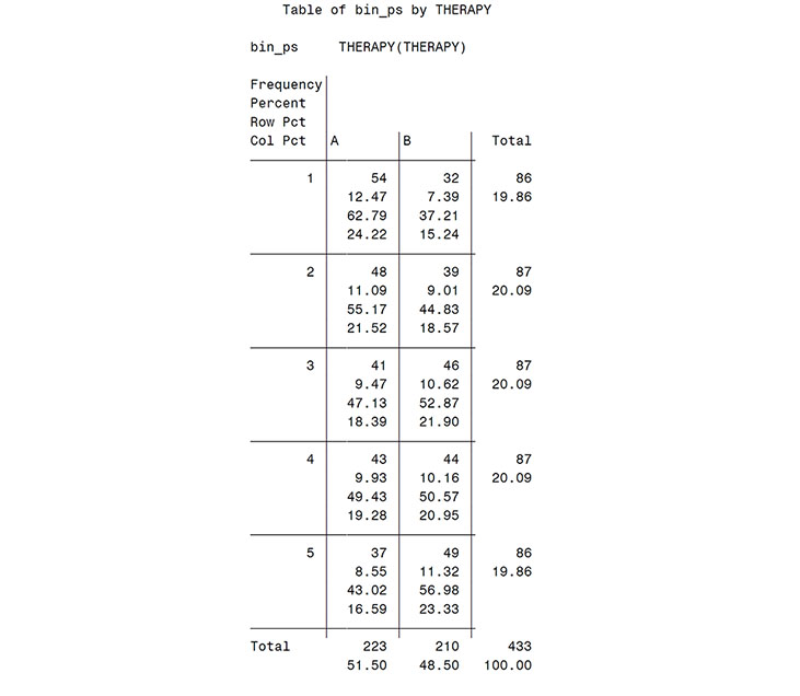
proc freq data = rankmab;
tables bin_ps*therapy;
title 'Therapy distribution among bins';
run;
proc tabulate data = rankmab;
class therapy bin_ps;
var respdays totcost;
tables bin_ps*therapy,(respdays totcost)*(n*format=3. mean std);
title 'Summary of costs/responder days by bin and therapy';
run;
/*******************************************************************
Macro PSBB is for a propensity score bin bootstrap analysis
Inputs:
REP = Number of bootstrap samples
AVARC = Variable for Total Costs
AVARE = Variable for Effectiveness (response days calculated for BPRS)
INDAT = Data set to be analyzed
GRPVAR = Variable for therapy group number
FSEED0 = Starting randomization seed for therapy group 0
FSEED1 = Starting randomization seed for therapy group 1
********************************************************************/
%MACRO
PSBB(rep=, avarc=, avare=, indat=, grpvar=, fseed0=887583, fseed1=566126);
data temp; set &indat;
run;
proc freq data=temp noprint;
tables &grpvar / out=freqnums;
where not(&grpvar=.);
run;
data _null_; set freqnums;
call symput('val'||compress(put(_n_, 4.)), trim(left(&grpvar)));
call symput('ssize'||compress(put(_n_, 4.)), trim(left(count)));
run;
%* Create data sets for each treatment *;
data trt0 trt1;
set temp;
if (&grpvar=&val1) then output trt0;
else if (&grpvar=&val2) then output trt1;
keep &grpvar &avarc &avare bin_ps;
run;
data bssumm; %* Empty data set to add to later *;
if _n_ eq 1 then stop;
run;
proc sort data=trt0; by &grpvar bin_ps;
run;
proc sort data=trt1; by &grpvar bin_ps;
run;
%do i=1 %to &rep;
%** Generate random bootstrap sample data set for therapy0**;
%* Perform bootstrap resampling *;
%let btnum=%qsysfunc(round(&ssize1/5,1));
%let rseed=%qsysfunc(round(&i + &fseed0, 1));
proc surveyselect data=trt0 method=urs outhits rep=1
n=&btnum. seed=&rseed. noprint out=trt0out;
strata &grpvar bin_ps;
run;
%** Generate random bootstrap sample data set for therapy1**;
%let btnum=%qsysfunc(round(&ssize2/5,1));
%let rseed=%qsysfunc(round(&i + &fseed1, 1));
proc surveyselect data=trt1 method=urs outhits rep=1
n=&btnum. seed=&rseed. noprint out=trt1out;
strata &grpvar bin_ps;
run;
data bothgrps;
set trt0out trt1out;
run;
%** Compute overall statistics for the sample **;
proc means data=bothgrps noprint;
class &grpvar;
var &avarc &avare;
output out = mn mean = out_avgc out_avge;
data mn; set mn end=eof;
label &avarc._avg1 = "Average for &AVARC, Group=&VAL1"
&avare._avg1 = "Average for &AVARE, Group=&VAL1"
&avarc._avg2 = "Average for &AVARC, Group=&VAL2"
&avare._avg2 = "Average for &AVARE, Group=&VAL2";
dumm= 1;
retain &avarc._avg1 &avare._avg1 &avarc._avg2 &avare._avg2;
if &grpvar=0 then do;
&avarc._avg1=out_avgc;
&avare._avg1=out_avge;
end;
if &grpvar=1 then do;
&avarc._avg2=out_avgc;
&avare._avg2=out_avge;
end;
keep dumm &avarc._avg1 &avare._avg1 &avarc._avg2 &avare._avg2;
if eof then output;
run;
%** Update data set with statistics from this sample **;
data bssumm;
set bssumm mn;
run;
%**Clean work library**;
proc datasets library=work memtype=data nolist;
delete trt0out trt01ut bothgrps mn;
run;
quit;
%end; %* End of %do loop *;
%** Compute differences and test statistics **;
data bssumm;
set bssumm;
&avare._diff = &avare._avg2 - &avare._avg1;
&avarc._diff = &avarc._avg2 - &avarc._avg1;
if &avarc._diff ne . and &avare._diff ne . then do;
if &avarc._diff ge 0 and &avare._diff ge 0 then ce_quad = '++';
if &avarc._diff ge 0 and &avare._diff lt 0 then ce_quad = '+-';
if &avarc._diff lt 0 and &avare._diff ge 0 then ce_quad = '-+';
if &avarc._diff lt 0 and &avare._diff lt 0 then ce_quad = '--';
end;
if &avarc._diff lt (&mc2 - &mc1) then zzeroctc + 1;
if &avare._diff lt (&me2 - &me1) then zzerocte + 1;
label &avare._diff="Average for &AVARE Diff: Grp2-Grp1"
&avarc._diff="Average for &AVARC Diff: Grp2-Grp1";
run;
*Calculate quadrants percentage and assign macro variable for graph **;
ods output OneWayFreqs=quadrt(keep=ce_quad percent);
proc freq data = bssumm;
tables ce_quad;
title2 "Quadrants distribution for cost effectiveness";
title3 "Variables &avarc and avare";
run;
data null_; set quadrt;
if ce_quad='++' then call symput('pospos', compress(percent));
if ce_quad='+-' then call symput('posneg', compress(percent));
if ce_quad='-+' then call symput('negpos', compress(percent));
if ce_quad='--' then call symput('negneg', compress(percent));
run;
proc univariate data=bssumm freq noprint;
var &avarc._diff &avare._diff;
output out=pctls pctlpts=2.5 97.5 pctlpre = &avarc &avare
pctlname=_lcl _ucl;
run;
proc print data=pctls;
title2 "Bootstrap Percentile 95% confidence limits for &avarc and
&avare"; run;
** Compute BCa confidence intervals **;
data zerodat;
set bssumm;
by dumm;
if last.dumm;
keep zzeroctc zzerocte;
run;
data bcacalc;
set zerodat;
zzeroc = probit( zzeroctc / &rep );
zzeroe = probit( zzerocte / &rep );
zzl = probit(.025);
zzh = probit(.975);
bcaclo = zzeroc + ((zzeroc + zzl) / (1 - &c_aconst.*(zzeroc + zzl)));
bcachi = zzeroc + ((zzeroc + zzh) / (1 - &c_aconst.*(zzeroc + zzh)));
bcaelo = zzeroe + ((zzeroe + zzl) / (1 - &e_aconst.*(zzeroe + zzl)));
bcaehi = zzeroe + ((zzeroe + zzh) / (1 - &e_aconst.*(zzeroe + zzh)));
bcacl = probnorm(bcaclo);
bcach = probnorm(bcachi);
bcael = probnorm(bcaelo);
bcaeh = probnorm(bcaehi);
run;
data _null_; set bcacalc;
call symput('bcacl', trim(left(bcacl*100)));
call symput('bcach', trim(left(bcach*100)));
call symput('bcael', trim(left(bcael*100)));
call symput('bcaeh', trim(left(bcaeh*100)));
run;
%put bcacl=&bcacl bcach=&bcach bcael=&bcael baceh=&bcaeh;
proc univariate data=bssumm freq noprint;
var &avarc._diff;
output out=pctls2 pctlpts=&bcacl. &bcach. pctlpre = &avarc
pctlname=_lcl _ucl;
run;
proc print data=pctls2;
title2 "BCa bootstrap 95% confidence limits for &avarc";
run;
proc univariate data=bssumm freq noprint;
var &avare._diff;
output out=pctls3 pctlpts=&bcael. &bcaeh. pctlpre = &avare
pctlname=_lcl _ucl;
run;
proc print data=pctls3;
title2 "BCa bootstrap 95% confidence limits for &avare";
run;
%** Create graph of bootstrap ce **;
axis1 label=(h=1.5 c=black a=90 "Effectiveness Difference: A - B"
J=CENTER) value=(h=1.5 c=black) ;
axis2 label=(h=1.5 c=black "Cost Difference: A - B" J=CENTER)
value=(h=1.5 c=black) ;
proc gplot data=bssumm;
plot &avare._diff*&avarc._diff = '*'/nolegend haxis=axis2
vaxis=axis1
href=0
vref=0 ;
%**Add quadrant frequency percentage **;
note height=1.75 m=(80pct,80pct) "&pospos.%";
note height=1.75 m=(80pct,30pct) "&posneg.%";
note height=1.75 m=(20pct,30pct) "&negneg.%";
note height=1.75 m=(20pct,80pct) "&negpos.%";
title1 h=2.5 lspace=1 "Quadrant distribution for cost effectiveness";
run; quit;
%**Clean work library**;
proc datasets library=work memtype=data nolist;
delete temp freqnums trt0 trt1 pctls pctls2 pctls3 zerodat;
run; quit;
goptions reset=all;
%MEND PSBB; /* End of macro psbb */
/* Call the bootstrap macro */
filename myfile1 "D:TempICER_TOTCOST_RDBPRS_DIFF2.gif";
goptions reset=all device=gif gsfname=MYFILE1 gsfmode=replace htext=1 ftext=swiss rotate=landscape noborder;
%PSBB(rep=10000,avarc=totcost,avare=respdays,indat=rankmab,grpvar=ther);
quit;
goptions reset=all;
***Draw histogram of mean difference in costs***;
data bssumm; set bssumm;
totcost_diff1=totcost_diff/1000;
**resize the cost to show in the graph x-axis**;
run;
filename myfile2 "D:TempICER_TOTCOST_DIFF2.gif";
goptions reset=all device=gif gsfname=MYFILE2 gsfmode=replace htext=1.25 ftext='arial/bo' rotate=landscape noborder;
title ' ';
footnote ' ';
pattern1 v=solid c=black;
footnote1 h=1.5 "Mean Difference in Costs: A - B (thousand $)";
AXIS1 LABEL=(H=2 C=BLACK angle=90 "Frequency" J=CENTER) value=(H=1.5
C=BLACK) order=(0 to 1600 by 200);
AXIS2 LABEL=(H=2 C=BLACK J=CENTER ' ') ;
PROC GCHART data=bssumm;
VBAR totcost_diff1/ref=(0 to 1600 by 200) midpoints=(-12 to 12 by 1) raxis=axis1 maxis=axis2 space=5 width=2;
run; quit;
goptions reset=all;
PROC PRINTTO; RUN;
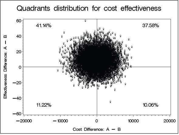
With a small estimated cost savings and a small effectiveness advantage, the point estimate of incremental cost-effectiveness does fall within the dominant region (save $173 with a gain of 9 days of response; not a tradeoff here). Output from Program 14.2 confirms that, relative to its uncertainty, this ICE point estimate is quite near the origin. In fact, the bootstrap distribution of ICE uncertainty spans all four quadrants of the cost-effectiveness plane. Note that one has 41.1% confidence in dominance (indicating better effectiveness and less cost for treatment A), 37.6% in the “A is more costly and more effective” quadrant, and 10%-12% in each of the other two quadrants (“A is less costly and less effective” and “A is more costly and less effective”). Thus, Obenchain and his colleagues’ (2005) levels of confidence needed to signal some, much, or strict dominance are not met in this example.
While not presented in detail here, sensitivity analyses utilizing other methods demonstrated some striking results in regard to treatment comparisons of costs. While the simple t-test (p=.900) and generalized linear model (gamma distribution) (p=.880) provided similar results to the PSBB analysis, both a log-transformation analysis (p=.007) and a Wilcoxon-ranked sum test (p=.045) resulted in statistically significant lower costs for the treatment B group. This is despite the fact that the observed mean costs were higher for this group. This is a result of the fact that in this situation the log-transformed and ranked tests are not reliable tests for differences in means. The median was lower for treatment B—as picked up by the ranked test—and a simple comparison of the variances of the log-transformed data (as can be obtained through PROC TTEST) demonstrates that the assumptions behind the log-transformed analysis are not valid here. Gianfrancesco and colleagues (2002) have discussed the potential for situations such as this, especially when comparing costs for treatments from different medication classes.
In this chapter, we have discussed the main issues involved in analyzing cost and cost-effectiveness comparisons between groups. SAS code for performing a PSBB analysis was provided along with a simulated example based on a schizophrenia trial. The PSBB approach is an attractive analytical method because it assesses the mean costs, is nonparametric, and adjusts for baseline selection bias through the well-accepted approach of propensity score stratification. PSBB may not be the best method for all situations—as comparative research on methodology to understand under what scenarios various methods perform best is lacking.
We have not fully addressed all issues involved in either the analysis or the presentation of cost data. First, we focused here on the statistical analysis methodology—ignoring issues such as study design, collection of resources or costs, assignment of costs to resource data, and cost discounting—because these have been widely discussed in the referenced guidelines on economic analyses. We also have not discussed the effects of missing or censored cost data. The methods illustrated here assume that unbiased cost estimates or imputed values are available or that the methods for addressing the missing data can be used within the structure of the propensity score bin bootstrap analysis (for example, use a method that adjusts for censoring [such as described in Chapter 16] to estimate cost differences within each propensity stratum—instead of a simple mean difference within each stratum as presented here). For other references on dealing with missing data specific to cost analyses, see Willan and Briggs (2006) or Young (2005). In addition, we did not present a full discussion of issues and options surrounding cost-effectiveness approaches (see Chapter 15).
Our objectives here were to use a specific example to illustrate that propensity score bin bootstrapping is relatively easy for researchers to implement and to demonstrate the importance of understanding the basic assumptions behind statistical methods for analysis of cost data. Given the variety of methods available, the different assumptions necessary for the different methods to be valid, the fact that different results follow from the same data using different methods, and the importance of cost analyses to health care payer decision-makers, what should outcomes researchers do? We contend that quality analyses and presentation of cost data must include at least the following three components:
1. a thorough assessment of the reasonableness of all assumptions made and the implications if the assumptions are not met;
2. documented proof that sensitivity analyses were performed; and
3. transparency in reporting all results.
Studies by Obenchain and Johnstone (1999) and Kereiakes and colleagues (2000) are two good examples of quality cost and cost-effectiveness analyses in this sense.
Bouckaert, A., and R. Crott. 1997. “The difference in mean costs as a pharmacoeconomic outcome variable: power considerations.” Controlled Clinical Trials 18: 58–64.
Briggs, A. H., D. E. Wonderling, and C. Z. Mooney. 1997. “Pulling cost-effectiveness analysis up by its bootstraps; a non-parametric approach to confidence interval estimation.” Health Economics 6(4): 327–340.
Chernick, M. R. 1999. Bootstrap Methods––A Practitioner’s Guide. New York: John Wiley & Sons, Inc., p. 264.
D’Agostino, Jr., R. B. 1998. “Propensity score methods for bias reduction in the comparison of a treatment to a non-randomized control group.” Statistics in Medicine 17: 2265–2281.
Davies, L. M., S. Lewis, P. B. Jones, T. R. E. Barnes, F. Gaughran, K. Hayhurst, A. Markwick, H. Lloyd, and the CUtLASS team. 2007. “Cost-effectiveness of first- v. second-generation antipsychotic drugs: results from a randomised controlled trial in schizophrenia responding poorly to previous therapy.” British Journal of Psychiatry 191(1): 14–22.
DiCiccio, T. J., and B. Efron. 1996. “Bootstrap confidence intervals.” Statistical Science 11: 189–228.
Doshi, J. A., H. A. Glick, and D. Polsky. 2006. “Analyses of cost data in economic evaluations conducted alongside randomized controlled trials.” Value in Health 9(5): 334–340.
Drummond, M., R. Brown, A. M. Fendrick, P. Fullerton, P. Neumann, R. Taylor, and M. Barbieri, Marco; the ISPOR scientific task force. 2003. “Use of pharmacoeconomics information––report of the ISPOR task force on the use of pharmacoeconomic/health economic information in health-care decision making.” Value in Health 6(4): 407–416.
Duan, N. 1983. “Smearing estimate: a nonparametric retransformation method.” Journal of the American Statistical Association 78: 605–610.
Duggan, M. 2005. “Do new prescription drugs pay for themselves? The case of second-generation antipsychotics.” Journal of Health Economics 24(1): 1–31.
Garrison, Jr., L. P., P. J. Neumann, P. Erickson, S. Marshall, and C. D. Mullins. 2007. “Using real-world data for coverage and payment decisions: the ISPOR Real-World Data task force report.” Value in Health 10(5): 326–335.
Gianfrancesco, F., R. Wang, R. Mahmoud, and R. White. 2002. “Methods for claims-based pharmacoeconomic studies in psychosis.” PharmacoEconomics 20(8): 499–511.
Grimes, D. A., and K. F. Schulz. 2002. “Bias and causal associations in observational research.” The Lancet 359: 248–252.
Kereiakes, D. J., R. L. Obenchain, B. L. Barber, A. Smith, M. McDonald, T. M. Broderick, J. P. Runyon, T. M. Shimshak, J. F. Schneider, C. R. Hattemer, E. M. Roth, D. D. Whang, D. Cocks, and C. W. Abbottsmith. 2000. “Abciximab provides cost- effective survival advantage in high-volume interventional practice.” American Heart Journal 140(4): 603–610.
Lindsey, J. K., and B. Jones. 1998. “Choosing among generalized linear models applied to medical data.” Statistics in Medicine 17: 59–68.
Liu, G. G., S. X. Sun, D. B. Christensen, and Z. Zhao. 2007. “Cost analysis of schizophrenia treatment with second-generation antipsychotic medications in North Carolina’s Medicaid program.” Journal of the American Pharmacists Association 47(1): 77–81.
Lumley T., P. Diehr, S. Emerson, and L. Chen. 2002. “The importance of the normality assumption in large public health data sets.” Annual Review of Public Health 23: 151–169.
Manning, W.G. 1998. “The logged dependent variable, heteroscedacsticity, and the retransformation problem.” Journal of Health Economics 17: 283–295.
Mullahy, J. 1998. “Much ado about two: reconsidering retransformation and the two-part model in health econometrics.” Journal of Health Economics 17(3): 247–281.
Nyhuis, A. W., M. D. Stensland, and D. E. Faries. 2003. “Calculating responder days for cost- effectiveness studies.” Schizophrenia Research 60(1) (Supplement 1): 341.
Obenchain, R. L. 2003-2006. “ICEpsbbs: a Windows application for incremental cost-effectiveness inference via propensity score bin boot strapping (two biased samples).” Available at http://members.iquest.net/~softrx/ICErefs.htm
Obenchain, R. L., and B. M. Johnstone. 1999. “Mixed-model imputation of cost data for early discontinuers from a randomized clinical trial.” Drug Information Journal 33: 191–209.
Obenchain, R. L., C. A. Melfi, T. W. Croghan, and D. P. Buesching. 1997. “Bootstrap analyses of cost effectiveness in antidepressant pharmacotherapy.” PharmacoEconomics 11(5): 464–472.
Obenchain, R. L., R. L. Robinson, and R. W. Swindle. 2005. “Cost-effectiveness inferences from bootstrap quadrant confidence levels: three degrees of dominance.” Journal of Biopharmaceutical Statistics 15(3): 419–436.
Oostenbrink, J. B., and M. J. Al. 2005. “The analysis of incomplete cost data due to dropout.” Health Economics 14(8): 763–776.
Polsky, D., H. A. Glick, R. Willke, and K. Schulman. 1997. “Confidence intervals for cost-effectiveness ratios: a comparison of four methods.” Health Economics 6(3): 243–252.
Polsky, D., J. A. Doshi, M. S. Bauer, and H. A. Glick. 2006. “Clinical trial based cost-effectiveness analyses of antipsychotic use.” The American Journal of Psychiatry 163: 2047–2056.
Ramsey, S., R. Willke, A. Briggs, R. Brown, M. Buxton, A. Chawla, J. Cook, H. Glick, B. Liljas, S. Petitti, and S. Reed. 2005. “Good research practices for cost-effectiveness analysis alongside clinical trials: the ISPOR RCT-CEA task force report.” Value in Health 8(5): 521–533.
Revicki, D. A., and L. Frank. 1999. “Pharmacoeconomic evaluation in the real world: effectiveness versus efficacy studies.” PharmacoEconomics 15(5): 423–434.
Rosenbaum, P. R., and D. B. Rubin. 1983. “The central role of the propensity score in observational studies for causal effects.” Biometrika 70: 41–55.
Rosenbaum, P. R., and D. B. Rubin. 1984. “Reducing bias in observational studies using subclassification on a propensity score.” Journal of the American Statistical Association 79: 516–524.
Rosenheck, R., D. Perlick, S. Bingham, W. Liu-Mares, J. Collins, S. Warren, D. Leslie, E. Allan, E. C. Campbell, S. Caroff, J. Corwin, L. Davis, R. Douyon, L. Dunn, D. Evans, E. Frecska, J. Grabowski, D. Graeber, L. Herz, K. Kwon, W. Lawson, F. Mena, J. Sheikh, D. Smelson, and V. Smith-Gamble; Department of Veterans Affairs Cooperative Study Group on the Cost-Effectiveness of Olanzapine. 2003. “Effectiveness and cost of olanzapine and haloperidol in the treatment of schizophrenia: a randomized controlled trial.” The Journal of the American Medical Association 290(20): 2693–2702.
Rosenheck, R. A., D. L. Leslie, J. Sindelar, E. A. Miller, H. Lin, T. S. Stroup, J. McEvoy, S. M. Davis, R. S. Keefe, M. Swartz, D. O. Perkins, J. K. Hsiao, and J. Lieberman; CATIE Study Investigators. 2006. “Cost-effectiveness of second-generation antipsychotics and perphenazine in a randomized trial of treatment for chronic schizophrenia.” The American Journal of Psychiatry 163(12): 2080–2089.
Roy-Byrne, P. P., C. D. Sherbourne, M. G. Craske, M. B. Stein, W. Katon, G. Sullivan, A. Means-Christensen, and A. Bystritsky. 2003. “Moving treatment research from clinical trials to the real world.” Psychiatric Services 54(3): 327–332.
Rutten-van Mölken, M. P., E. K. van Doorslaer, R. C. van Vliet. 1994. “Statistical analysis of cost outcomes in a randomized controlled clinical trial.” Health Economics 3(5): 333–345.
Tollefson, G. D., C. M. Beasley, Jr., C.M. Jr., P. V. Tran, J. S. Street, J.S., J. A. Krueger, R. N. Tamura, K. A. Graffeo, and M. E. Thieme. 1997. “Olanzapine versus haloperidol in the treatment of schizophrenia and schizoaffective and schizophreniform disorders: results of an international collaborative trial.” The American Journal of Psychiatry 154(4): 457–465.
Tunis, S. L., D. E. Faries, A. W. Nyhuis, B. J. Kinon, H. Ascher-Svanum, and R. Aquila. 2006. “Cost-effectiveness of olanzapine as first-line treatment for schizophrenia: results from a randomized, open-label, 1-year trial.” Value in Health 9(2): 77–89.
Willan, A. R., and A. H. Briggs. 2006. Statistical Analysis of Cost-Effectiveness Data. West Sussex, England: John Wiley & Sons Ltd., p. 196.
Young, T. A. 2005. “Estimating mean total costs in the presence of censoring: a comparison assessment of methods.” PharmacoEconomics 23(12): 1229–1242.
Zhu, B., S. L. Tunis, Z. Zhao, R. W. Baker, M. J. Lage, L. Shi, and M. Tohen. 2005. “Service utilization and costs of olanzapine versus divalproex treatment for acute mania: results from a randomized, 47-week clinical trial.” Current Medical Research and Opinion 21(4): 555–564.