
Chapter 6
Face Biometric Data Indexing
Face-based biometric identification system with a large pool of data requires huge computation time to search an individual’s identity from database due to the high dimensionality of the face biometric features. In this work, a new indexing technique is proposed for face-based biometric identification system to narrow down the search space. The technique is based on the Speed Up Robust Feature (SURF) key points and descriptors [10]. Index keys are generated for a face image from the key points and descriptors of the face image. A two level index space is created based on the extracted key points. A storing and retrieving techniques have been proposed to store and retrieve the face data to or from the proposed index space. Figure 6.1 gives an overview of the proposed approach.
The rest of the chapter is organized as follows. Different steps of preprocessing technique for face image will be outlined in Section 6.1. The feature extraction methodology for face will be discussed in Section 6.2. Index key generation method for face biometric will be presented in Section 6.3. The storing and retrieving techniques for face data shall be given in Section 6.4 and Section 6.5, respectively. Performance of the proposed method with different face databases will be analyzed in Section 6.6. Section 6.7 will present the comparison with existing work. The chapter will be concluded in Section 6.8.

Figure 6.1: An overview of the proposed face biometric data indexing approach.
6.1 Preprocessing
Input face image of a biometric system contains background and is usually of not good quality. To extract the features from a face image, the background is needed to remove and the image quality should be enhanced. This makes feature extraction task easy and also ensures the quality of the extracted features. Some essential preprocessing tasks is required to follow for the above mentioned reason. The steps followed in the preprocessing are described in the following.
6.1.1 Geometric Normalization
All input face images may not be of same size and aligned in the same direction (e.g. due to the movement of head at the time of capturing). Geometric normalization process proposed by Blome et al. [13] and Beveridge et al. [12] is followed to align and scale the images so that the face images are in the same position, same size and at the same orientation. To get geometric normalized image, first, the eye coordinates are searched from the face image using Blome et al. [14, 15] method. Let (XL, YL) and (XR, YR) be the detected left and right eye coordinates, respectively.The angle (θ) between horizontal axis and the line passing through the two eye coordinates is calculated as shown in Fig. 6.2(a). The angle θ is calculated using Eq. (6.1).

To lines up the eye coordinates, the image is rotated by −θ angle. Let I(x’, y’) be transformed image of I(x, y) after rotation by −θ angle. The rotated image is shown in Fig. 6.2(b). Transformation relation between original image pixel and resultant image pixel is given in Eq. (6.2).

After rotating the face image, the face part is detected from the rotated image. To do this, Viola and Jones’s [30] face detection algorithm is used. A snapshot of the detected face is shown in Fig. 6.2(c). To make the face image scale invariant, the detected face part (DW × DH ) is mapped into a fixed size image (FW × FH) by applying scaling transformation. The scaling factor s is calculated using Eq. (6.3).
In this approach, F H = 150 and FW = 130 are considered, because, in general, aspect ratio of a face image would be 1.154 [13]. The detected image is wrapped into fixed size image by applying translation and followed by scaling. Let I (x, y) and I(x”, y”) be the detected and fixed size face image. The transformation is done using Eq. (6.4). In Eq. (6.4), (tx, ty) is the top left coordinate of the detected face image (see Fig. 6.2(c)). Figure 6.2(d) shows the fixed image of width FW and height FH.

6.1.2 Face Masking
Masking is the process of separating the foreground region from the background region in the image. The foreground region correspond to the clear face area containing the significant feature value, which is called the area of interest. The masking is done to ensure that the face recognition system does not respond to features corresponding to background, hair, clothing etc. An elliptical mask [13, 12] is used such that only the face from forehead to chin and cheek to cheek is visible. Let (xc, yc) is the center of the elliptical mask which is just below the eye level. The following mathematical model [13] is applied to each face image to mask the background region.

Figure 6.2: Face images after different preprocessing tasks.
Let I(x,y) be the detected face image obtained after geometric normalization. The masked image I’(x, y) is calculated as per the following rule.

where, a and b are minor axis and major axis of elliptical shape, respectively. Figure 6.2(e) shows the face image after applying mask on geometric normalized image where only face part is present in the image and the background has been masked out.
6.1.3 Intensity Enhancement
Intensity enhancement is required to reduce the variations due to lighting and sensor differences. The intensity enhancement is done in two steps [13]. First, the histogram of the unmasked face part is equalized and then the intensity of the image is normalized to a mean of zero and standard deviation of one.
To equalize the histogram of an image, the cumulative distribution (cdf ) of the histogram is calculated. The cdf at each gray level v represents the sum of its occurrence and the occurrence of the previous gray level in image. Then the histogram equalization is done by Eq. (6.5).
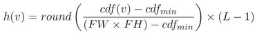
where cdfmin is the minimum value of the cumulative distribution function, FW and FH are the width and height of image, and L is the number of gray levels used.
Next, the intensity values of the equalized face image is normalized. Intensity normalization is used to standardize the intensity values in an image by adjusting the range of gray level values so that it lies within a desired range of values. Let I(i, j) represents the gray level value at pixel (i, j) of histogram equalized image and N(i, j) represents the gray level value at pixel (i, j) in normalized image. The normalization is done using Eq. (6.6).

where M and V are the estimated mean and variance of I(i, j), respectively, and M0 and V0 are the desired mean and variance values, respectively. The pixel values is selected to have a mean of zero and a standard deviation of one in the experiment. Figure 6.2(f) shows the intensity enhancement image of the geometric normalization image.
6.2 Feature Extraction
Speed Up Robust Feature (SURF) [9, 10] method is known as a good image interest points (also called key points) and feature descriptors detector. SURF method is applied in this approach. This method is used because it has several advantages over other feature extraction methods. The most important property of an interest point detector using SURF method is its repeatability. Repeatability means that the same interest points will be detected in different scales, orientations and illuminations of a given image. Another advantage is that the SURF method is computationally very fast. In addition to these, the SURF feature provides scale, rotation and illumination invariant feature descriptors.
The feature extraction method consists of three different tasks: key point detection, orientation assignment and key point descriptor extraction. In this section, first the different steps of the key point detection method is presented. The orientation assignment of each key point is discussed next. Then the method of feature descriptor extraction at each key point is described.
6.2.1 Key Point Detection
Bay et al. [9, 10] method is followed to detect key points from a face image. The method is based on Hessian matrix approximation [10] which uses integral images to reduces the computation time of key points detection. The method consists of three steps. First, the scale space of the preprocessed image is created, which helps to detect key points at different scales of the image. Next, Hessian matrix [23, 10] is calculated at each pixel position in the different scale space images and the value of the determinant of the Hessian matrix is computed. Note that all detected key points are not necessarily discriminant because the determinant of the Hessian matrix does not produce local maximum or minimum response at all detected points. Hence, the most discriminant key points are localized from all detected key points. In the following, the detailed descriptions of the above mentioned steps are presented.
6.2.1.1 Scale Space Creation
Scale space of an image is represented by an image pyramid as shown in Fig. 6.3(a). To create an image pyramid, a fixed size Gaussian filter is applied to an image and then sub sampled filtered image [19]. This process should be done repeatedly to get the higher layered images of a scale space. Since, the repeated sub sampling of image demands more computation time, this is done in a different way. A Gaussian filter is applied into the image keeping the image size fixed but increasing the filter size (see Fig. 6.3(b)). This gives the same result of decreasing the size of image and finds Gaussian convolution using same size of filter and then scale up the image due to the cascading properties of Gaussian filter [19, 10].
Scale space is made of number of octaves; where an octave represents a series of filter responses obtained by convolving the same input image with doubling the filter size. Again, an octave is divided into a constant number of scale levels. To create scale space Bay et al. [10] method is followed. Eight distinct Gaussian filters are constructed with different sizes and different standard deviations. The Gaussian filter of size m × m and standard deviation σ is represented as Gm×m(σm). The eight Gaussian filters are G9×9(σ9), G15×15(σ15), G21×21(σ21), G27×27(σ27), G39×39(σ39), G51×51(σ51), G75×75(σ75) and G99×99(σ99) (for details please see the reference [10]). Base level of scale space is created with filter size 9 × 9 and standard deviation (σ) 1.2 (also referred as scale s=1.2). Next, scale spaces are obtained by changing the size of filter. As the filter size is changed to obtain subsequent scale space the associate Gaussian scale is needed to change as well so that ratios of layout remain constant. This standard deviation (scale) of current filter can be calculated using Eq. (6.7).

Figure 6.3: Approaches to scale space creation.
In Eq. (6.7), σc and σb be the standard deviation of current filter and base filter, respectively, and Sizec and Sizeb denote the current filter size and base filter size, respectively.
6.2.1.2 Hessian Matrix Creation
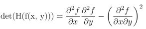
SURF detector [10] is based on determinant of Hessian matrix [23, 10]. Blob-like structures which differ in properties like brightness or color compared to the surrounding are detected at locations where the determinant of Hessian matrix is maximum. Let f (x, y) be a function of two variables, then Hessian matrix H is defined as in Eq. (6.8).

Hence, determinant of above matrix will be as follow:
(6.9)
The maxima and minima can be computed from the above determinant formula. This will help to classify the points into maxima and minima based on the sign of result. Let x (x, y) be a point in an image I(x, y). Then Hessian matrix is calculated as follows.

(6.10)
Here, ![]() ,
, ![]() and
and ![]() . Further, Lxx(x, σm) represents the convolution
of the Gaussian second order derivative of Gaussian filter at scale σm with the image I(x, y) at point x; similarly the Lxy(x, σm) and Lyy(x, σm). These entire derivatives are known as Laplacian of Gaussian [19]. The determinant of each pixel is calculated to find the interest points.
. Further, Lxx(x, σm) represents the convolution
of the Gaussian second order derivative of Gaussian filter at scale σm with the image I(x, y) at point x; similarly the Lxy(x, σm) and Lyy(x, σm). These entire derivatives are known as Laplacian of Gaussian [19]. The determinant of each pixel is calculated to find the interest points.
To reduce the computation time of calculating Laplacian of Gaussian, Bay et al. approximation method [10] is followed. The approximation of the Laplacian of Gaussian is done using box filter representations of the respective Gaussian filters. Figure 6.4 shows the weighted box filter approximations of discretized and cropped second order Gaussian derivatives in the x, y and xy-directions. Suppose, Dxx, Dyy and Dxy represent the weighted box filter response [10] of the second order Gaussian derivatives Lxx, Lyy and Lxy, respectively. Then Hessian determinant with box filter approximation is calculated using Eq. (6.11) [10].
The above determinant value is referred to as the blob response at location x = (x, y) with scale σm. This method of Hessian matrix creation is applied for each point of each scale space for a face image.
6.2.1.3 Key Point Localization
Key points are detected based on the determinant value of the Hessian matrix. As the high determinant value at a point represents more discriminant [9] point, those points are considered where the determinant values are high. For this reason, first, a threshold value is chosen and the points whose values are less than the threshold are removed. Bay et al. [9] show that the threshold value 600 is good for detecting the discriminant key point from an image with average contrast and sharpness. In this experiment, the threshold value is chosen as 600. Next, non-maximal suppression [19] is performed to find the candidate key points. To do this, each point of scale space is compared with its 26 neighbors (see Fig. 6.5) and the local maxima is found. Eight points are considered from the scale space at which non-maximal suppression is done and 9 points from both above and below the scale space of that. Finally, to localize key points the maxima of the determinant of the Hessian matrix is interpolated in scale and image space. To do this, the method proposed by Brown and Lowe [16] is used.

Figure 6.4: Gaussian partial 2nd order derivative and their approximation.
6.2.2 Orientation Assignment
An orientation is assigned to each key point to extract rotation invariant features from the input face image. The orientation is important because the feature descriptors are extracted relative to this orientation in later stage. To find the orientation of a key point, first, a circular area centered with the key point of radius 6σ is created where σ is the standard deviation of the Gaussian filter [10] at the current scale space. Then, the Haar wavelet response [20] is calculated at each point within the circular area in x and y directions. Haar filter of size 4σ is used. The Haar filter responses in x and y directions are calculated using two filters as shown in Fig. 6.6(a) and (b). Then, weighted response of Haar wavelet response is calculated with Gaussian filter. The Gaussian filter is centered with interest point and the value σ of Gaussian is taken as 2. The weighted responses are represented by points in vector space as shown in Fig. 6.6(c). To find dominating orientation, the resultant vector in window of size 60 degree is computed as shown in Fig. 6.6(c). The longest vector is taken as the orientation of that key point.

Figure 6.5: Non-maximal suppression by checking the nearest neighbor in subsequent scale spaces.
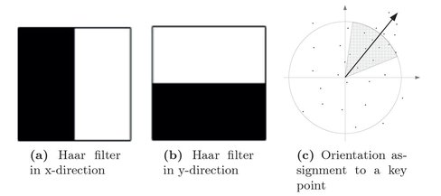
Figure 6.6: Haar filters in x- and y- directions and orientation of a key point.

Figure 6.7: SURF descriptor extraction at a key point.
A set of key points is detected from an image and orientation of each key point is estimated. A key point can be represented with position, orientation, scale space in which the key point is detected, Laplacian value and the determinant of Hessian matrix. Let k1, k2, . . ., kL be the L detected key points of an input image. The key points of an image is represented as shown in Eq. (6.12).

In Eq. (6.12), (x, y) and θ represent the position and orientation of a key point, respectively; σ (σ ∈ σ9, σ15, σ21, σ27, σ39, σ51, σ75, σ99) denotes scale space at which key point is detected (see Section 6.2.1.1); ls and hs represent the Laplacian value and determinant of Hessian matrix, respectively.
6.2.3 Key Point Descriptor Extraction
In this step, the feature descriptors are extracted at each key point from the scale space images as follows. Scale space images are created
by applying Gaussian filter on the images (as discussed in Section 6.2.1.1). SURF method [10] is followed to extract the feature descriptors from the face image. First, a square window of size 20σ is created where σ is the scale or standard deviation of the Gaussian filter at which key point is detected. The window is centered at key point position and the direction of window is the same with the orientation of the key point (see Fig. 6.7). Now, the window is divided into 4 × 4 square sub regions and within each sub-region 25 (5 × 5) regularly distributed sample points are placed. Haar wavelet responses [20] is calculated at each sample point of a sub-region in x and y directions. The Haar wavelet responses are weighted with a Gaussian filter with standard deviation 3.3σ centered at key point to reduce the effect of geometric deformations and localization errors. Let dx and dy be the Haar wavelet responses at each sample point within each sub-region. ∑ dx, ∑ |dx|, ∑ dy and ∑ |dy| are considered as four features at each sub-region. Hence, sixty four (4 × 4 × 4) descriptors are created corresponding to each key point. The extracted feature descriptors from a face image is shown in Eq. (6.13). In Eq. (6.13), d1, d2, . . . , di, . . . , dT represent descriptors of T key points and ![]() represents the jth descriptor of the ith key point.
represents the jth descriptor of the ith key point.

6.3 Index Key Generation
All key points and feature descriptors are extracted from all face images. A face image can be represented with a set of index keys. The
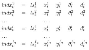
set of index keys are generated from the extracted key points of a face image such that for each key point there is an index key. More precisely, the key point information, feature descriptors and identity of a person are used as the constituents of an index key. An index key is represented as a row vector of sixty nine elements. The first four values of an index key contain the sign of Laplacian, position and orientation of a key point. Next sixty four values of the index key hold the feature descriptors corresponding to the key point and the last value keeps the identity of a person. The first four values are used to index the database and the feature descriptors are used to search the identity of a person. Suppose, there are P number of subjects and each has Q number of samples. Index keys for all samples of all subjects are generated. Let Tp,q be the number of key points ![]() and feature descriptors (
and feature descriptors (![]() ) extracted from the face image of the qth sample of the pth subject. Note that Tp,q may vary from one face image to another. Thus, Tp,q number of index keys are generated for the face image the qth sample of the pth subject. The index keys of the qth sample of the pth subject is presented in Eq. (6.14). The ith index key
) extracted from the face image of the qth sample of the pth subject. Note that Tp,q may vary from one face image to another. Thus, Tp,q number of index keys are generated for the face image the qth sample of the pth subject. The index keys of the qth sample of the pth subject is presented in Eq. (6.14). The ith index key ![]() of the qth sample of the pth subject is generated by the ith key point
of the qth sample of the pth subject is generated by the ith key point ![]() and corresponding feature descriptors
and corresponding feature descriptors ![]() , and the identity
, and the identity ![]() of the qth sample of the pth subject. In Eq. (6.14),
of the qth sample of the pth subject. In Eq. (6.14), ![]() ,
, ![]() ,
, ![]() ,
, ![]() and
and ![]() represent the sign of Laplacian, x and y positions, orientation and feature descriptors of the ith key point
represent the sign of Laplacian, x and y positions, orientation and feature descriptors of the ith key point ![]() , and
, and ![]() represents the identity of the face image of the qth sample of the pth subject.
represents the identity of the face image of the qth sample of the pth subject.

6.4 Storing
Once all index keys are generated, the face data are to be stored into the database. To do this, first, a two-level index space is created in the database. Then the face data are stored into the index space in two ways: linear structure and kd-tree structure. The techniques of index space creation and storing are described in the following.
6.4.1 Index Space Creation
An index space needs to be created to store all index keys into the database. The created index space helps to find a match corresponding to a query in fast and accurate manner. To create index space, first four components of an index key are used. These are the sign of Laplacian (ls), positions (x and y) and orientation (θ) of a key point. All index keys can be classified into two groups based on the sign of the Laplacian value (ls) because this value distinguishes the brightness (dark and light) at a key point position. Note that all face images are aligned in the same direction and scaled to the same size in the preprocessing step. Hence, a key point will occur at the same or near to the same position in the image and the orientation of the key point will remain almost same although, the face images are captured at different time. So, the index keys in each group can be divided into sub-groups based on the positions (x and y) and orientation (θ) of a key point.
Due to the above characteristics of key points a two-level index space is proposed to store the index keys. In the first level, the index space is divided based on the value of ls of index keys. The value of ls can be either ‘−1’ for low intensity value or ‘+1’ for high intensity value for a key point. Hence, the first level index space (LS) is divided into two sub-index spaces (LS1 and LS2) as shown in Fig. 6.8. In the second level, each sub-index space is divided into a number of cells based on the positions (x and y) and orientation (θ) of key points. The second level index space (INDX) is represented as a three dimensional index space. The three dimensions of index space are x, y and θ. Each dimension is in different scales. To bring each dimension in the same scale, each dimension is normalized. To do this, each dimension of the second level index space is quantized into the same number of units. Each dimension is quantized into δ number of units. The value of δ is decided experimentally (discussed in Section 6.6.3). Each three dimensional index space in the second level is refered as an index cube. Each index cube contains δ3 number of cells. Figure 6.8 shows two three-dimensional index cubes for storing the index keys.

Figure 6.8: Proposed index space to store all index keys of all face images.
Now, all index keys are stored into the index space based on the first four values of the index keys. Note that a number of index keys may map into a single cell of an index cube because index values of a set of index keys may fall within the same range. The cell positions are found for all index keys. To do this a set of hash functions are defined based on the sign value of Laplacian, positions and orientation of a key point. Let ls, (x, y) and θ be the sign value of Laplacian, positions and orientation of a key point, respectively. Then the hash functions are defined in Eq. (6.15). In Eq. (6.15), ls’, x’, y’, and θ’ are the normalized cell index of the two-level index space and FH and FW represent the height and width of the normalized face image, respectively.

The storing of an index key into the proposed two-level index space is illustrated with an example. Let indx =< ls = −1, x = 55,y = 89, θ = 45, ƒd1, ƒd2, . . . , ƒd64, Id > be an index key of a face image of size 130 × 150 (FW × FH ) , ƒd1 to ƒd64 are the 64 feature descriptors of that key point and Id be the identity of the subject. To store the feature descriptors (ƒd1, ƒd2, . . . , ƒd64) and the identity (Id) into the index space, the hash functions (defined in Eq. (6.15)) are applied on ls, x, y and θ of the key point. The feature descriptors will be stored into the first index cube (LS1) of the first level of index space because the value of ls’ is 1 after applying the hash function on ls. The cell position of the index cube in second level index space (INDX) is decided by applying the hash function on x,y and θ. Let assume that each dimension of second level index space is divided into 15 units (i.e. δ = 15). After applying the hash function on x, y and θ the value of x’, y’ and θ’ are 7, 9 and 2, respectively. Hence, the feature descriptors (ƒd1, ƒd2, . . . , ƒd64) and identity (Id) of the index key (indx) is stored at [7,9,2] location in the first index cube which is represented as LS1 → INDX[7][9][2].
It may be noted that a cell of an index cube can contain a set of feature descriptors and identities of index keys. To store the feature descriptors and identities of index keys, two storing structures: linear storing structure and kd-tree storing structure have been proposed. These storing structures are discussed in the following.
6.4.2 Linear Storing Structure
In this technique, a 2-D linear index space (LNINDX) is created for each cell of the index cube. Each linear index space is assigned a unique identity (lid) and this identity is stored into the corresponding cell of the index cube. Note that there are δ3 number of cells in each index cube. Hence, 2δ3 number of linear index spaces are created to store all index keys using linear storage structure. The linear index space (LNINDX) stores the 64-dimensional feature descriptors (f d1, f d2, . . . , f d64) and identities (Id) of index keys. Figure 6.9 shows the linear index space (LNINdXi) for the ith cell of the first index cube (LS[1] → INDX). The cell stores the identity (lidi) of the linear index space (LNINDXi). The ith cell of the index cube LS[1] → INDX is represented as CELL[i]. All index keys of the ith cell are stored into the linear index space (LNINDXi). Hence, the size of the linear index space (LNINDXi ) is Ni × (64 + 1) where Ni is the number of index keys in the ith cell and an index key contains 64-dimensional feature descriptor. The method for creating linear index space is summarized in Algorithm 6.1. In Step 7 of Algorithm 6.1, the index cube are found from the first level index space. The cell position of the index cube is found in Step 8 to Step 10. Step 11 calculates the identity of linear index space and Step 12 assigns that identity to a cell of an index cube. The descriptor values and the identities of index keys are found in Step 13 and 14.
6.4.3 Kd-tree Storing Structure
A kd-tree is created for each cell of an index cube and assign a unique identity (kid) to each kd-tree. The identity of the kd-tree is stored into the corresponding cell of the index cube. There are 2δ3 number of cells in the index space. Hence, the total number of kd-trees required is 2δ3. All index keys of a cell are stored into a kd-tree. A kd-tree is a data structure for storing a finite set of points from a k-dimensional space [8, 7, 25] and the structure is defined in Section 5.4.3.

Figure 6.9: Linear index space to store all index keys of the ith cell.
All sixty four dimensional points (descriptors of an index key) are stored within a cell into a kd-tree data structure. Kd-tree insertion method is applied to store the index keys. This method is proposed by Arya and Mount [7, 8] which follows Bentley [11] kd-tree insertion method. The maximum height of the optimized kd-tree with N number of k-dimensional point is ⌊log2(N )⌋ [11]. The kd-tree structure for the ith cell is shown in Fig. 6.10. In Fig. 6.10, KDINDXi is the kd-tree for the ith cell of the first index cube (LS[1] → INDX). The cell stores the identity (kidi) of the ith kd-tree (KDINDXi). The ith cell of the first index cube LS[1] → INDX is represented as CELL[i]. The method for creating kd-tree index space is summerized in Algorithm 6.2. Step 7 of Algorithm 6.2 finds the position of first level index space and Step 8 to Step 10 calculate the cell position in the index cube. Step 11 calculates the unique identity of the kd-tree. The identity of the kd-tree is assigned into a cell of an index cube in Step 12. Finally, the descriptor values and the identity of a subject are inserted into the kd-tree in Step 15.
Algorithm 6.1 Creating index space with linear storing structure

6.5 Retrieving
Querying is the process of retrieving a set of candidates from the enrolled face templates corresponds to a query template. The retrieved templates are most likely to match with the query face template. Two different searching techniques have been investigated to retrieve the face templates from the database of two different storage structures discussed previously. In each searching technique, first the index keys are generated corresponding to the query face using index key generation technique (discussed in Section 6.3). Let the index keys generated from a query face are represented in Eq. (6.16).
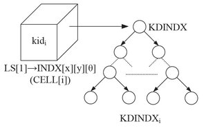
Figure 6.10: Kd-tree to store the index keys of the ith cell of the index space.
The ith query index key is represented as ![]() , where
, where ![]() ,
, ![]() ,
, ![]() and
and ![]() ,
, ![]() represent the sign of Laplacian, x and y position, orientation, feature descriptor of the ith key point (
represent the sign of Laplacian, x and y position, orientation, feature descriptor of the ith key point (![]() ) of the query face image, respectively. Then, indexing is applied on the first level index space using the value of ls of the query index key. The indexing is done using hash functions defined in Eq. (6.15). The first level of indexing selects the index cube for a query index key. Let assume that the value of ls of the ith index key of query is −1. Then index cube (LS[1] → INDX) in the first level index space (LS) is selected for the ith query index key. Next, hash functions (defined in Eq. (6.15)) are applied on the value of x, y and θ of the query index key to find the cell position of the index cube in the second level index space. Then, the candidate set (CSET ) is generated by counting the vote received for each identity of the retrieved index keys from the database. The CSET contains two fields: id and vote. The id and vote fields of the CSET store the identities of subjects and the number of votes received for an identity. To generate the CSET, the linear or kd-tree structures are searched corresponding the identity stored in the selected cell of an index cube and find the closest match in the linear or kd-tree index space. If x, y and θ of the ith index key of a query select the LS[1] → INDX [x] [y] [θ] cell of the index cube LS[1] → INDX and retrieve the jth linear or kd-tree identity then the closest match is found in the LNINDXj linear index space for linear search and KDTREEj for kd-tree search. Finally, ranks are given based on the votes received by each identity. The search techniques are described in the following.
) of the query face image, respectively. Then, indexing is applied on the first level index space using the value of ls of the query index key. The indexing is done using hash functions defined in Eq. (6.15). The first level of indexing selects the index cube for a query index key. Let assume that the value of ls of the ith index key of query is −1. Then index cube (LS[1] → INDX) in the first level index space (LS) is selected for the ith query index key. Next, hash functions (defined in Eq. (6.15)) are applied on the value of x, y and θ of the query index key to find the cell position of the index cube in the second level index space. Then, the candidate set (CSET ) is generated by counting the vote received for each identity of the retrieved index keys from the database. The CSET contains two fields: id and vote. The id and vote fields of the CSET store the identities of subjects and the number of votes received for an identity. To generate the CSET, the linear or kd-tree structures are searched corresponding the identity stored in the selected cell of an index cube and find the closest match in the linear or kd-tree index space. If x, y and θ of the ith index key of a query select the LS[1] → INDX [x] [y] [θ] cell of the index cube LS[1] → INDX and retrieve the jth linear or kd-tree identity then the closest match is found in the LNINDXj linear index space for linear search and KDTREEj for kd-tree search. Finally, ranks are given based on the votes received by each identity. The search techniques are described in the following.

6.5.1 Linear Search
In linear search, first the cell position is found in an index cube for a query index key. Then, the linear index space of that cell is searched. Euclidean distance between feature descriptor of a query index key and all the feature descriptors stored in the linear index space is computed to find a match. Let the jth cell in the index cube is selected for the ith index key of a query. Then, the linear index space (CELL[j] → LNINDX) corresponding to the jth cell is selected to find a match. The Euclidean distances between the feature descriptors of the ith index key of the query and all the descriptors stored in the linear index space (CELL[j] → LNINDX) is computed using Eq. (6.17). The identity is retrieved corresponding to the minimum distance. The retrieved identity is then placed in the CSET and cast a vote for this identity. The same procedure is followed for all other index keys of the query face. The linear searching method is summarized in Algorithm 6.3. In Step 2 of Algorithm 6.3, the length of each linear index space is initialized. Step 6 and Step 7 to 9 find the index of the first and second level index spaces, respectively. The cell id is calculated in Step 10. In Step 11 to 19, the minimum distance for an index key of query face is found and the identity is retrieved corresponding to the minimum distance. Step 23 to 31 generate the CSET for a query index key. Finally, the CSET is sorted in Step 35.

Algorithm 6.3 Candidate set generation in linear search from index space


6.5.2 Kd-tree Search
In kd-tree search, first the cell position is found in an index cube for an index key of a query. Then the identity of a kd-tree (kid) is retrieved from the cell and search the kd-tree corresponding to the retrieved kd-tree identity. The hash functions are applied to find the cell position in the index cube. Let the jth cell in the index cube is selected for the ith query index key. Then kd-tree index space (CELL[j] → KDINDX) corresponding to the jth cell is searched to find a match. Approximate nearest neighbor search [7, 8, 26, 3] is applied to reduce the searching time. Arya and Mount’s [7, 3] approximate k nearest neighbor search method is used to search the kd-tree. In this technique, only the k closest bins of the kd-tree are examined and a priority queue is used to identify the closest bins based their distances from query. The expected searching complexity of the nearest neighbor search can be reduced to O (kdlogn) and space complexity is O (dn) . For this purpose, a public domain library (FLANN) [26, 3] for faster approximate nearest neighbors search is available. In the proposed approach, this library is utilized for implementing kd-tree algorithms. The identities corresponding to the closest match are retrieved from the kd-tree. The retrieved identities are then placed in the CSET and cast a vote for this identity. The same procedure is followed for all other index keys of the query face. The searching method for kd-tree index space is summarized in Algorithm 6.4. Step 3 and Step 4 to 6 of Algorithm 6.4 find the index of the first and second level index spaces, respectively. In Step 7, the cell identity of an index cube is calculated for a query index key. Step 8 finds the approximate nearest neighbors for a query index key and Step 9 retrieves the identities corresponding to the nearest neighbors. In Step 12 to 17, the CSET is generated for a query index key and sort the CSET in Step 20.


6.6 Performance Evaluation
The proposed method has been evaluated with different face databases in different experimental setups to measure the performance of face indexing approach. The performance metrics are defined in Section 4.7.1. In this section, first the face databases used in this experiment and then different experimental setups which are used are described. Then, experimental results observed in experiments with respect to the different performance metrics defined in Section 4.7.1 are presented. A comparison of the proposed approach with existing face indexing approaches is given in this section.
6.6.1 Database
The experiments are performed on two widely used large face databases, namely Color FERET [28, 2, 5] and FRGC V2.0 [27, 29, 4]. The experiments are also carried out on CalTech 256 [18, 1] face database. Detailed description of each database is given in the following.
Color FERET Face Database: The FERET database is developed for the Facial Recognition Technology (FERET) program [2, 5]. The database is designed by the Defense Advanced Research Products Agency (DARPA) [5] during 1993 to 1997 to give common standard for face recognition experiments. The database contains 11338 images from 994 different subjects. These images are collected in different sessions. The resolution of the captured images is 256 × 384 pixel. The database contains 2722 frontal images with different facial expressions (Neutral and Alternate). There are 1364 images with neutral expression and 1358 images with alternate expression. Figure 6.11(a) and (b) shows the four images with different facial expressions of two different subjects.
FRGC 2.0 Face Database: FRGC Still version 2.0 data set [27, 29, 4] is collected at University of Notre Dame as a part of Face Recognition Grand Challenge (FRGC) program. The primary goal of the FRGC program is to promote and advance the face recognition technology. This database contains color face images, which are taken in different lightning conditions and environments. The database consists of 24038 frontal face images of 466 subjects. These images are captured in Fall 2003 and Spring 2004 semesters of 2003-2004 academic year. A total of 16024 images from all subjects are captured in indoor environment with two different protocols (FERET and Mugshot) and two different facial expressions (Neutral and Smiley) [27]. The resolution of each image is either 1704 × 2272 pixel or 1200 × 1600 pixel. The images are collected in 4007 subject sessions. Four images (FERET-Neutral, FERET-Smiley, Mugshot-Neutral and Mugshot-Smiley) are captured in each subject session. The database contains 4007 FERET-Neutral, 4007 FERET-Smiley, 4007 Mugshot-Neutral and 4007 Mugshot-Smiley face images. Figure 6.11(c) and (d) shows four images with two facial expressions of two different subjects. FRGC Still version 2.0 data set [27, 29, 4] contains 8014 face images which are captured in outdoor environment with different backgrounds and illuminations. Figure 6.11(e) shows two face images of two different subjects in different backgrounds.

Figure 6.11: Sample images from FERET, FRGC and CalTech256 databases.
CalTech 256 Face Database: Caltech-256 object category data set [1, 18] contains a total of 30607 images from 256 different categories. In this experiment, face category images of the Caltech-256 data set are used. The face category set consists of 432 face images from 28 subjects. Each face image is captured in complex background with different facial expressions. Figure 6.11(f) shows two face images of two different subjects from CalTech 256 face database.
6.6.2 Evaluation Setup
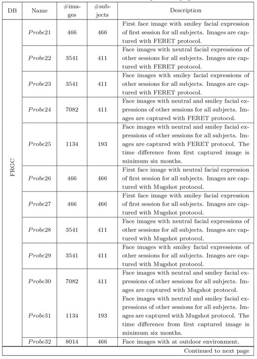
To evaluate the proposed indexing method, each face database is partitioned into two sets: Gallery and Probe. The Gallery set contains the face images which are enrolled into the index database and Probe set contains the face images which are used as queries to search the index database. In this experiment, different Gallery and Probe sets are created for each database. The descriptions of different Gallery and Probe sets for FERET, FRGC and CalTech256 databases are given in Table 6.1.
All methods described in this approach are implemented using C programming language and OpenCV [6] image processing library in the Linux operating system. All methods are evaluated with Intel Core-2 Duo processor of speed 2.00GHz and 2GB RAM.
Table 6.1: Description of Gallery and Probe sets of FERET, FRGC and CalTech256 face databases.


6.6.3 Validation of the Parameter Value
The experimental results reported in this chapter are subjected to the validity of the value of the parameter used. The value of dimension quantization of the second level index space (δ) is considered as an important parameter in this experiment. The validity is assessed on the basis of experimental evaluation of the variable. The value of δ is validated in the following.
To determine the value of the number of quantization (δ) of each dimension of the second level index space, the following experiment has been done. Kd-tree based search is performed for a set of query images with different values of δ. The value of δ is varied from 2 to 50 with increment of 2. This experiment is conducted with FERET, FRGC and CalTech databases. Gallery11 and Probe11 for FERET database, Gallery21 and ProbeP21 for FRGC database, and Gallery41 and Probe41 for CalTech database are used for this experiment. The rank one HR and PR for different values of δ as observed are shown in Fig. 6.12. From Fig. 6.12(a), it is observed that for FERET database rank one H R decreases nearly 2% when the value of δ is changed 2 to 14 whereas rank one H R decreases more than 4% when the value of δ is changed 16 to 20. On the other hand, the P R decreases more than 85% when the value of δ is changed 2 to 14 but P R decreases only 5% for the change of δ value 14 to 20 for FERET database. The similar trend is observed for FRGC database also (see Fig. 6.12(b)). On the other hand, the value of δ equal to 12 gives better performance than the other values of δ for Caltech database (see Fig. 6.12(c)). Hence, in other experiments, the value of δ equal to 15 is chosen for FERET and FRGC databases, and 12 for Caltech database, respectively. However, user may choose the other values of δ according to their requirements.

Figure 6.12: HR and PR with FERET, FRGC and CalTech256 databases for different values of δ.
6.6.4 Evaluation
A number of experiments have been conducted to evaluate the accuracy, searching time and memory requirement of the proposed face indexing method. The descriptions of these experiments and the result of each experiment are given in the following.
6.6.4.1 Accuracy
The accuracy is measured with respect to H R, P R and C M S metrics. In the first experiment, the performance of the proposed method with and without applying indexing is shown. Next, the performances of the proposed indexing method with different Probe sets is presented. The effect of multiple number of samples enrollment into the database is shown in the next experiment. Finally, the FPIR and FNIR are measured for the face-based identification system with the proposed indexing technique.
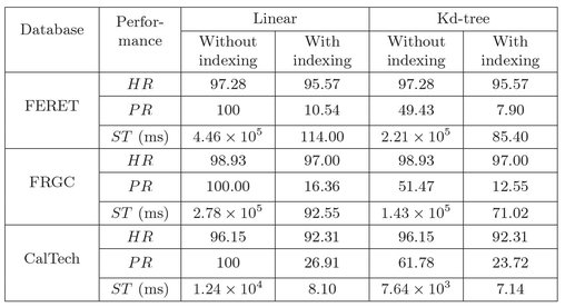
Performances with and without indexing: In this experiment, the performance of the system with and without applying the proposed indexing technique is compared. Gallery11 and Probe11 for FERET, Gallery21 and Probe21 for FRGC databases, and Gallery41 and Probe41 for CalTech databases are used in this experiment. The CMC curves with and without indexing for different databases are shown in Fig. 6.13. Figure 6.13(a) shows that the approach without indexing gives better cumulative match score for FERET database. Whereas, from Fig. 6.13(b) and (c), it can be seen that the approach with and without indexing gives almost the same CMS after the 15 th rank for FRGC database and after the 7th rank for CalTech database. The rank one H R, P R and average searching time (ST) are reported for linear and kd-tree search using indexing and without indexing in Table 6.2. From Table 6.2, it can be seen that kd-tree search with indexing achieves 95.57%, 97% and 92.31% H R with 9.70%, 12.55% and 7.14% P R for FERET, FRGC and CalTech databases, respectively. It is also observed that kd-tree search requires less average searching time for all three databases.

Figure 6.13: CMC curve with and without indexing for FERET, FRGC and CalTech256 databases.
Performance with different probe sets: In this experiment, the performances of linear and kd-tree search have been checked with the proposed indexing method for different Probe sets. The Probe sets are created with different conditions as discussed in Table 6.1. The all images of Gallery11 (with neutral expression), Gallery21 (with neutral expression) and Gallery41 are enrolled into the database for FERET, FRGC and CalTech databases, respectively and all probe sets are used to test the indexing performances of linear and kd-tree search. Figure 6.14(a), (b) and (c) show the CMC curves of all probe sets of FERET, FRGC, CalTech256 databases, respectively. From Fig. 6.14(a) and (b), it can be noted that the CMSs are reduced for the Probe sets which contain the face images captured in more than six month difference. On the other hand, face images captured with different expressions but in the same session give the better results than the others. It is observed that face images with complex background (Probe32 of FRGC database) give less CMS than the others. However, face images with complex background for CalTech database give above 90% CMS. The rank one HR, P R and ST for linear and kd-tree search for different Probe sets are given in Table 6.3. It is observed that the P R and ST for kd-tree based search are less for all Probe sets.
Table 6.2: Performance of the proposed approach with and without indexing using linear and kd-tree search
Performance of multiple enrollments of a subject into the index space: The experiment has been done to check the effect of multiple enrollments on the performance. In this experiment, all samples of Gallery12 for FERET, Gallery22 for FRGC and Gallery42 for CalTech databases are enrolled, and all Probe sets of FERET, FRGC and CalTech databases are used for testing. The CMC curves of all Probe sets are shown in Fig. 6.15. From Fig. 6.15, it can be seen that 100% CMS is achieved for Probe11 and Probe21 because the images in the Probe11 and Probe21 sets are also in the Gallery12 and Gallery22, respectively. It is observed that in multiple enrollments of a subject, CMSs for other probe sets are increased than that of the single enrollments. The P R, rank one H R and searching time for linearand kd-tree based search is computed with multiple enrollments. The results are summarized in Table 6.4. From this experiment, it is observed that better rank one HR is achieved without affecting the PR. Nevertheless, a higher searching time is required to search the database with multiple enrollments.

Figure 6.14: CMC curves for different Probe sets with single enrolment of a subject with FERET, FRGC and CalTech256 databases.
Table 6.3: Performance of different Probe sets with single enrolment of a subject in linear and kd-tree search


Figure 6.15: CMC curves for different Probe sets with multiple enrolment of a subject with FERET, FRGC and CalTech256 databases.
FPIR and FNIR: The performance of the proposed system is analyzed with respect to FPIR and FNIR. Gallery11, Gallery21 and Gallery42 sets are used as Gallery sets, and Probe11, Probe21 and Probe43 are used as Probe sets for FERET, FRGC and CalTech databases, respectively. There are 992, 466 and 1297 genuine scores and 985056, 216690 and 27403 imposter scores are computed for FERET, FRGC and CalTech databases, respectively. The trade-off between FPIR and FNIR for the identification system without indexing and with indexing is shown in Fig. 6.16. The equal error rates (EER) of the system without indexing are 6.38%, 5.12% and 15.78% for FERET, FRGC and CalTech databases, respectively. Whereas, the EERs with indexing are 6.06%, 4.87% and 14.36% for FERET, FRGC and CalTech databases, respectively.
Table 6.4: Performance of different Probe sets for multiple enrolments of a subject in linear and kd-tree search

6.6.4.2 Searching Time
The time complexities of linear and kd-tree based search techniques are analyzed in the proposed index space. Let N be the total number of face images enrolled in the database and Tp be the average number of index keys in each enrolled face image. Thus, the total number of index keys in the index space is Tn = Tp × N . If there are K number of cells in all index cubes, then the average number of index keys in each cell is Tk = Tn/K . Let Tq be the average number of index keys in each query face image. To perform linear search or kd-tree based search in the index space, first, the index cell position is found for an index key of a query using hash functions defined in Eq. (6.15). This operation requires O(1) computation time for both type of searching. The time complexity analysis of linear and kd-tree based searching within the located cell are given in the following.

Figure 6.16: FPIR vs. FNIR curve with and without indexing for FERET, FRGC and CalTech256 databases.
Linear search: In linear search, Tk × Tq number of comparisons are required to retrieve a set of similar index keys and their identities, and Tq log Tq comparisons are required to sort the retrieved identities based on their ranks. Thus, the average time complexity of linear search (denoted as TLS ) can be calculated as follows.

Kd-tree search: The number of comparisons required in kd-tree based search to find a set of nearest index keys and their identities are log Tk × Tq , and to sort the retrieved identities based on their ranks are Tq log Tq . Thus, the average time complexity of kd-tree based search (denoted as TKS ) can be calculated as follows.

(6.19)
The searching time and the average number of comparisons required for linear and kd-tree based search techniques is calculated with the proposed index space. To compute these, different number of samples are enrolled into the index space for FERET, FRGC and CalTech databases. The execution time (in Intel Core-2 Duo 2.00 GHz processor and 2GB RAM implementation environment) of linear and kd-tree search with FERET, FRGC and CalTech databases are shown in Fig. 6.17(a), (b) and (c), respectively. It is observed that the execution time for kd-tree search is less than the linear search method. It is also observed that the rate of increment in execution time for kd-tree based search is less when the number of enrolled sample increases. The average number of comparisons for linear and kd-tree based search is given in Fig. 6.18. From Fig. 6.18, it can be seen that the rate of increment in number comparisons is also less for kd-tree based search. Hence, it may be concluded that to retrieve the similar identities for a given query, kd-tree based search within index cell is better than the linear search.

Figure 6.17: Average searching time with different sizes of databases for FERET, FRGC and CalTech256 databases.
6.6.4.3 Memory Requirement
Here, the memory requirement is analyzed for two proposed storing structures. Let b1 and b2 bytes memory are required to store the reference of the index cubes into the first level index space and the reference of linear or kd-tree index spaces into the index cube, respectively. Let m bytes are required to store a feature value of an index key and 2 bytes are required to store an identity of a subject. If there are P subjects and each subject has Q samples then the memory requirement for linear and kd-tree index spaces can be computed using Eq. (6.20) and (6.21), respectively. In Eq. (6.20) and (6.21), Tp,q represents the number of index keys of the qth sample of the pth subject and δ denotes the number of quantization levels of the second level index space.

Figure 6.18: Average number of comparisons with different sizes of databases for FERET, FRGC and CalTech256 databases.

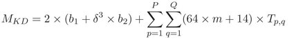
(6.21)
In this approach, 2 bytes are required to store the reference of index cube into a cell of first level index space and 4 bytes are required to store the reference of linear or kd-tree index space into a cell of index cube. There are 64 feature values in an index key and 4 bytes are required to store a feature value. The identity of a subject is also stored with each index key. The identity field requires 2 bytes extra memory for each index key. 216 identities can be stored with 2 bytes identity field. Hence, a total of 258 bytes are required to store an index key along with the identity in linear index space. In kd-tree based index space, a single node of kd-tree requires 270 bytes memory. Figure 6.19(a), (b) and (c) show the memory requirements for linear and kd-tree index spaces to store different number of samples for FERET, FRGC and CalTech databases, respectively. From Fig. 6.19, it is observed that the memory requirements are almost same for the linear and kd-tree based index spaces.

Figure 6.19: Memory requirements with different sizes of databases for FERET, FRGC and CalTech256 databases.
6.7 Comparison with Existing Work
The proposed approach is compared with three existing face indexing approaches [22, 24, 21]. To compare the proposed work, Gallery11, Gallery21 and Gallery41 are used as Gallery sets, and Probe11, Probe21 and Probe41 are used as Probe sets for FERET, FRGC and CalTech databases, respectively. The comparison result is reported in Table 6.5. The comparison is done with respect to rank one HR, P R and average searching time (ST). From Table 6.5, it can be seen that the approach gives better performance than the existing approaches.
Table 6.5: Comparison of the proposed approach with existing approaches

6.8 Summary
In this chapter, an approach of creating a two-level indexing mechanism is discussed for a face biometric-based identification system. The work has been published in [17]. The proposed indexing mechanism reduces search space for face-based identification system. In this technique, a set of sixty nine dimensional index keys is created using SURF feature extraction method from a face image. Among sixty nine dimensions, only four dimensions are considered to create the two-level index space. In the first level of indexing, the index keys are grouped based on the sign of Laplacian value and in the second level, the index keys are grouped based on the position and the orientation. A set of similar identities for a query are found from the two-level index space using a hashing technique. The hashing technique requires O(1) time complexity to retrieve the identities. Linear and kd-tree based searching mechanism have been explored to search the identities within the two-level index space. The approach is tested with FERET, FRGC and CalTech face databases. The experimental result shows that kd-tree based search performs better than the linear search. On an average 95.57%, 97% and 92.31% rank one HR with 7.90%, 12.55% and 23.72% PR can be achieved for FERET, FRGC and CalTech databases, respectively. Further, this approach gives better HR when multiple samples of a subject are enrolled into the database. On the average 8.21%, 11.87% and 24.17% search space reduction are possible for different probe sets of FERET, FRGC and CalTech, respectively. With the proposed indexing approach, the computation time advantage can be achieved without compromising the accuracy compared to traditional face-based person identification systems. The limitations of the proposed approach is that it does not give good results under different poses (e.g. left or right profile) of face images.
Bibliography
- [1] CalTech 256. CalTech 256 Face Database. URL http://www.vision.caltech.edu/Image_Datasets/Caltech256/ . (Accessed on October, 2012).
- [2] FERET. The Facial Recognition Technology (FERET) Database. URL http://www.itl.nist.gov/iad/humanid/feret/feret_master.html . (Accessed on December, 2011).
- [3] FLANN - Fast Library for Approximate Nearest Neighbors. URL http://www.cs.ubc.ca/~mariusm/index.php/FLANN/FLANN . (Accessed on May, 2012).
- [4] NIST FRGC. Face Recognition Grand Challenge (FRGC). URL http://www.nist.gov/itl/iad/ig/frgc.cfm. (Accessed on May, 2012).
- [5] NIST FERET. The Color FERET Database: Version 2. URL http://www.nist.gov/itl/iad/ig/colorferet.cfm. (Accessed on February, 2012).
- [6] OpenCV. The Open Source Computer Vision (OpenCV) Library. URL http://opencv.willowgarage.com/wiki/Welcome. (Accessed on December, 2011).
- [7] S. Arya and D. M. Mount. Algorithms for Fast Vector Quantization. In Proceedings of DCC ’93: Data Compression Conference, pages 381–390, Snowbird, UT, 1993.
- [8] S. Arya, D. M. Mount, N. S. Netanyahu, R. Silverman, and A. Y. Wu. An Optimal Algorithm for Approximate Nearest Neighbor Searching in Fixed Dimensions. Journal of the ACM, 45(6):891–923, 1998.
- [9] H. Bay, T. Tuytelaars, and L. V. Gool. SURF: Speeded Up Robust Features. In Proceedings of the 9th European Conference on Computer Vision, volume LNCS-3951, pages 404–417, Graz, Austria, May 2006. doi: http://dx.doi.org/10.1007/11744023_32.
- [10] H. Bay, A. Ess, T. Tuytelaars, and L. V. Gool. SURF: Speeded Up Robust Features. Computer Vision and Image Understanding , 110(3):346–359, 2008. doi: http://dx.doi.org/10.1016/j.cviu. 2007.09.014.
- [11] J. L. Bentley. Multidimensional Binary Search Trees Used for Associative Searching. Communications of the ACM, 18(9):509–517, 1975. ISSN 0001-0782. doi: http://dx.doi.org/10.1145/361002. 361007.
- [12] J. R. Beveridge, D. Bolme, B. A. Draper, and M. Teixeira. The CSU Face Identification Evaluation System. Machine Vision and Applications, 16(2):128–138, 2005. doi: http://dx.doi.org/10.1007/s00138-004-0144-7 .
- [13] D. S. Bolme, J. R. Beveridge, M. L. Teixeira, and B.A. Draper. The CSU Face Identification Evaluation System: Its Purpose, Features and Structure. In Proceedings of the 3rd International Conference on Computer Vision Systems, pages 304–313, Graz, Austria, April 2003.
- [14] D. S. Bolme, J. R. Beveridge, and B. A. Draper. FaceL: Facile Face Labeling. In Proceedings of the 7th International Conference on Computer Vision Systems, volume LNCS-5815, pages 21–32, Liège, Belgium, October 2009. doi: http://dx.doi.org/10.1007/978-3-642-04667-4_3 .
- [15] D. S. Bolme, B. A. Draper, and J. R. Beveridge. Average of Synthetic Exact Filters. In Proceedings of the Computer Vision and Pattern Recoginition, pages 2105–2112, Miami, Florida, June 2009.
- [16] M. Brown and D. G. Lowe. Invariant Features from Interest Point Groups. In Proceedings of the British Machine Vision Conference, pages 656–665, Cardiff, Wales, September 2002.
- [17] J. Dewangan, S. Dey, and D. Samanta. Face images database indexing for person identification problem. International Journal of Biometrics and Bioinformatics (IJBB), 7(2):93–122, 2013.
- [18] G. Griffin, A. Holub, and P. Perona. Caltech-256 Object Category Dataset. Technical report, California Institute of Technology, Pasadena, CA, USA, 2007.
- [19] R. Jain, R. Kasturi, and B.G. Schunck. Machine Vision. McGraw-Hill Inc, New York, 1st edition, 1995.
- [20] A. Jensen and A. L. Cour-Harbo. Ripples in Mathematics: The Discrete Wavelet Transform. Berlin, Heidelberg. Springer-Verlag, 1st, 2001.
- [21] V. D. Kaushik, A. K. Gupta, U. Jayaraman, and P. Gupta. Modified Geometric Hashing for Face Database Indexing. In Proceedings of the 7th international conference on Advanced Intelligent Computing Theories and Applications: with Aspects of Artificial Intelligence, pages 608–613, Zhengzhou, China, August 2011.
- [22] K. H. Lin, K. M. Lam, X. Xie, and W. C. Siu. An Efficient Human Face Indexing Scheme using Eigenfaces. In Proceedings of the IEEE International Conference on Neural Networks and Signal Processing, pages 920–923, Nanjing, China, December 2003.
- [23] T. Lindeberg. Feature Detection with Automatic Scale Selection. International Journal of Computer Vision, 30(2):79–116, 1998. doi: http://dx.doi.org/10.1023/A:1008045108935.
- [24] P. Mohanty, S. Sarkar, R. Kasturi, and P. J. Phillips. Subspace Approximation of Face Recognition Algorithms: An Empirical Study. IEEE Transactions on Information Forensics and Security , 3(4):734–748, 2008.
- [25] Andrew Moore. A Tutorial on Kd-trees. Technical report, University of Cambridge, 1991. URL http://www.cs.cmu.edu/~awm/papers.html .
- [26] M. Muja and D. G. Lowe. Fast Approximate Nearest Neighbors with Automatic Algorithm Configuration. In Proceedings of the International Conference on Computer Vision Theory and Applications (VISAPP’09), pages 331–340, 2009.
- [27] J. Phillips and P. J. Flynn. Overview of the Face Recognition Grand Challenge. In Proceedings of the IEEE Conference on Computer Vision and Pattern Recognition, pages 947–954, San Diego, USA, June 2005.
- [28] P. J. Phillips, H. Moon, S. A. Rizvi, and P. J. Rauss. The FERET Evaluation Methodology for Face-Recognition Algorithms. IEEE Transactions on Pattern Analysis and Machine Intelligence, 22 (10):1090–1104, 2000. doi: http://dx.doi.org/10.1109/34.879790.
- [29] P. J. Phillips, P. J. Flynn, T. Scruggs, K. W. Bowyer, and W. Worek. Preliminary Face Recognition Grand Challenge Results. In Proceedings of the 7th International Conference on Automatic Face and Gesture Recognition, pages 15–24, Southampton, UK, April 2006.
- [30] P. Viola and M. J. Jones. Robust Real-time Face Detection. International Journal of Computer Vision, 57(2):137–154, 2004.