Chapter 8. Using spatial reference systems

This chapter covers

• Understanding spatial reference systems
• Transforming data using OSR
• Transforming data using pyproj
• Great-circle calculations using pyproj

Most people are familiar with the concept of using latitude and longitude to specify a location on the earth’s surface. Would you be surprised to learn that many other coordinate systems are also used, and that these different spatial reference systems are used for different purposes? To make things even more complicated, the earth isn’t a perfect sphere, and multiple models, called datums, are used to represent the planet’s shape. Given this, coordinates from any system, including latitude and longitude, aren’t absolute—a set of coordinates can specify a slightly different location depending on the datum used.

Because so many coordinate systems exist, it’s unlikely that all of your data will use the one you need, so the ability to convert data between them is critical. Not only that, but it’s impossible to transform data from one spatial reference system to another if you don’t know which system they currently use, so you must ensure that this information is documented or risk rendering your data unusable. To effectively work with coordinate systems, you need to understand why so many of them exist in the first place and how to select an appropriate one for your purposes, so we’ll start with background information and then move on to transforming data.

8.1. Introduction to spatial reference systems

A spatial reference system is made of three components—a coordinate system, a datum, and a projection—all of which affect where on the earth a set of coordinates refers to. Briefly, datums are used to represent the curvature of the earth, and projections transform coordinates from a three-dimensional globe to a two-dimensional map. Different projections are appropriate for different purposes, such as web mapping, accurately measuring distances, or calculating areas. There’s more to it than that, however, and it’s important to understand the role that both datums and projections play. Let’s back up and review how coordinates are represented on a globe. Latitude and longitude are the distance, in degrees, from the equator and the prime meridian, respectively. Latitude values range from -90 to 90, with positive values north of the equator. Longitudes range from -180 to 180, with positive values east of the Greenwich prime meridian (shown in figure 8.1). Using degrees makes perfect sense on a spherical surface, and although the earth isn’t a perfect sphere, it’s close enough for this to be a convenient way to specify a precise location on the planet.

Figure 8.1. Latitude and longitude lines at 30° intervals. Positive latitude values are north of the equator, and positive longitudes are east of the prime meridian.

Definition

The prime meridian is the line of longitude that passes through the Royal Observatory, Greenwich, in London. This has been recognized by much of the world as the reference meridian since 1884. The equator is the line of latitude that is equal distances from both the north and south poles.

However, a complication arises from the fact that the earth isn’t a perfect sphere or even a perfect ellipsoid. As you probably learned in geometry class, but then promptly forgot, simple equations can model the shape of ellipsoids, including spheres. But these equations assume a perfect geometry with a nice smooth surface and no protrusions and dips. It would be quite something if a planet were to form that perfectly, and ours certainly didn’t. Have you ever seen a worn-out ball, like a volleyball, that has developed a weak spot and has a bulge that wasn’t there when the ball was new? Not only does the earth have mountains and valleys, but it’s a little lopsided like that volleyball, which definitely makes describing its surface with a simple set of equations more complicated.

Because of these anomalies in the planet’s surface, and also because measurement accuracies vary, the earth’s ellipsoid has multiple models. These models are called datums, and every spatial reference system is based on one of them. One widely used global datum, the World Geodetic System, was last revised in 1984. This datum, called WGS84 for short, is the one used for data with a global coverage, including the Global Positioning System (GPS). Most datums are designed to model the curvature of the earth in a more localized area, such as a continent or even a smaller area. A datum designed for one area will not work well elsewhere. For example, the North American Datum of 1983 (NAD83) shouldn’t be used in Europe.

Depending on which datum is being used, the same set of latitude and longitude coordinates can refer to slightly different locations, because the underlying ellipsoids are different shapes. Sometimes the difference between coordinates using two different datums is negligible, but other times it can be hundreds of meters. Because of this, you always need to know which datum your geographic data is based on.

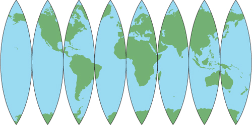
Until now we’ve only talked about three-dimensional ellipsoids, but what you really want in most cases is a two-dimensional map because they tend to be more convenient for most purposes. After all, it’s hard to fold up a globe and put it in your pocket or embed one inside of a book! How do mapmakers go from three to two dimensions? One way to solve the problem is with what’s called an interrupted map, like that shown in figure 8.2. You’ve probably seen these before, and perhaps you’ve even cut one out and bent the paper to make a globe. That’s kind of cool, but in its two-dimensional form, the map would be much easier to use if land masses weren’t split up into chunks and separated by wasted space. This is where projections come in. As their name implies, they’re used to project, or transform, locational data into a different coordinate system. These map projections use Cartesian coordinate systems, so locations are specified with x,y coordinate pairs based on two perpendicular axes, like scatterplots or line graphs. The tricky part is converting coordinates on a sphere to a two-dimensional plane.

Figure 8.2. An interrupted map

In fact, many ways to accomplish this exist, and they all have their own strengths and weaknesses. Think about stretching the different parts of the interrupted map shown in figure 8.2 so that the map was a single rectangle with no cutouts. Geographic features would obviously get warped, especially near the poles where you had to stretch farther. No matter how you project geographic data to two dimensions, you’ll get distortion, but the type of distortion depends on how you do the conversion. Depending on what you plan to use the data for, some types of distortion may be acceptable while others won’t. Figure 8.3 shows a couple of ways a piece of paper could be wrapped around a globe and used to convert the geographic data to 2D. Even with those methods shown here, the angle of the paper could be changed to get a different effect.

Figure 8.3. Two different ways that a piece of paper could be wrapped around a globe and used to project geographic data onto a two-dimensional surface. The example on the left is cylindrical, and the one on the right is conical.

Certain projections, called conformal, preserve local shapes. For example, the shape of Lake Titicaca on the border of Bolivia and Peru wouldn’t change between the globe and the 2D map. No mathematical trickery can preserve the shape of a large area, such as all of Eurasia, however. Mercator projections, including the Universal Transverse Mercator (UTM), are examples of conformal projections. Others, called equal-area projections, keep the amount of area the same, so the measured area of Greenland wouldn’t change, although the shape might. The Lambert equal-area and Gall-Peters projections are two examples of this. Equidistant projections, such as the Azimuthal equidistant, keep distances and scales the same, but only for a certain part of the map, such as the equator. The farther you get from this true line, the greater the distortion. Figure 8.4 shows examples of different projections.

Figure 8.4. Examples of different types of projections

Tip

Several terms exist for data that use latitude and longitude coordinate values. You might see them referred to as having a geographic projection or see them called unprojected or geographic.

Why should you care about all of these differences? Depending on your purposes, maybe you don’t. I doubt I’d be worried about it if I was making a map of the small town I live in. But if I was making a map of the state I live in, I might care if it looked short and fat or a little taller and skinnier, as shown in figure 8.5. What if you cared more about measurements and less about appearances? Let’s consider a dramatic example and think about what would happen if you needed to compare the amount of forested area in Columbia and Chile. Sticking with latitude and longitude wouldn’t work, because the lines of longitude converge at the poles, so one degree of longitude doesn’t represent a constant distance. In fact, one degree of longitude is equal to approximately 111 kilometers at the equator, but only about 79 km at a latitude of 45 degrees. Although latitude distance can vary slightly because the earth isn’t a perfect sphere, it’s generally around 111 kilometers per degree. Therefore, a square 100 km long on each side would measure about 0.8 square degrees in Columbia, but closer to 0.5 square degrees at the southern tip of Chile. Using latitude and longitude to compare the amount of forested area in the two countries would obviously give inaccurate results. Instead, you’d want to choose an appropriate equal-area projection for this purpose.

Figure 8.5. The state of Utah shown using geographic (lat/lon) coordinates on the left and UTM Zone 12N on the right. Both examples use the NAD83 datum.

Projections aren’t tied to specific datums, so knowing the projection of your data isn’t enough. You also need to know the datum, and it’s the combination of the two that defines the spatial reference system. For example, most of the data I get for Utah uses a UTM projection and the NAD83 datum, but I can’t safely assume that all UTM data I receive uses NAD83. It could easily be NAD27 or WGS84 instead, so I don’t have a complete spatial reference system unless I know both the projection and the datum. If you don’t know both components, you might map your data in the wrong location. I’ve known people who unknowingly set their GPS to display coordinates in an unusual spatial reference system and then collected data by writing down the coordinates shown on their screen. Unfortunately, their data were then unusable because they didn’t know what spatial reference system the GPS had been set to display at the time. On the other hand, I also know people who lacked spatial reference information for their data, but fortunately the data were in a common system and they figured it out. If you’re collecting data, please simplify your life by paying attention to this crucial information at the beginning of the process, no matter how boring it might seem.

Tip

If you collect geographic data, it’s crucial to know from the beginning what projection and datum your coordinates use. If you don’t pay attention to this, then your data may end up useless, and nobody wants that.

8.2. Using spatial references with OSR

Because spatial reference systems (SRSs) are so important, most vector data formats provide a way to store this information with the data, and you need to know how to work with it. When using spatial data, one common task is to convert the dataset from one spatial reference system to another so that it can be used with other datasets or for a particular analysis. The analysis techniques discussed in the last chapter, for example, only work if the geometries all use the same SRS. Another reason you might need to convert between SRSs is if you’re using an online mapping solution that requires a Web Mercator projection to display data.

Warning

Many GIS software packages will project on-the-fly, which means that they’ll automatically convert data to a different SRS when displaying it. For example, if you load in a dataset that uses an Albers equal-area projection, the map will be drawn using that projection. But if you then load a second file that uses UTM, it will be converted to Albers so it can be displayed correctly with the first. Of course, this only happens if both of the datasets have SRS information stored with them, because without that the software doesn’t know what to do. Also, this process only changes what’s in memory and doesn’t alter what’s stored on disk in any way. Although this behavior can be helpful when you’re using a GIS, sometimes it leads people to assume that datasets use the same SRS when in reality they don’t.

The osgeo package contains a module called OSR (short for OGR Spatial Reference) that’s used to work with SRSs. This section will show you how to use OSR to assign SRS information to your data so that GIS software, including OSR, knows how to work with it. You’ll also learn how to convert data between different SRSs so that you can transform data to whichever SRS you need for a particular project.

8.2.1. Spatial reference objects

To work with a spatial reference system, you need a SpatialReference object that represents it. If you already have a layer that uses the SRS you want, then you can get the SRS from it using the GetSpatialRef function. A similar function, GetSpatial-Reference, will get an SRS from a geometry. Both of these functions will return None if the layer or geometry doesn’t have an SRS stored with it.

Let’s look at the information contained in one of these SRS objects. Perhaps the easiest way is to print it out, which will display a nicely formatted description of the SRS in WKT format and doesn’t require the OSR module to be imported. The states_48 shapefile uses a geographic, or unprojected, coordinate system along with the North American Datum of 1983 (NAD83):

>>> ds = ogr.Open(r'D:osgeopy-dataUSstates_48.shp')
>>> print(ds.GetLayer().GetSpatialRef())
GEOGCS["GCS_North_American_1983",
    DATUM["North_American_Datum_1983",
        SPHEROID["GRS_1980",6378137.0,298.257222101]],
    PRIMEM["Greenwich",0.0],
    UNIT["Degree",0.0174532925199433]]

You can tell that this isn’t a projected SRS because it doesn’t have a PROJCS entry, only a GEOGCS one. If you were looking at a projected SRS, there would be more information describing the parameters of the coordinate system, such as the UTM example show in figure 8.6.

Figure 8.6. Well-known text for the NAD83 UTM Zone 12N spatial reference system

WKT isn’t the only string representation of an SRS. I like PROJ.4 strings because they’re especially concise. For example, this is the PROJ.4 string for the UTM SRS shown in figure 8.6:

'+proj=utm +zone=12 +ellps=GRS80 +towgs84=0,0,0,0,0,0,0 +units=m +no_defs '

The PROJ.4 Cartographic Projections Library is a popular open source library for converting data between projections, and you can read about the details of PROJ.4 definitions at http://trac.osgeo.org/proj/. See appendix D for other functions you can use to get text representations of spatial reference systems. (Appendixes C through E are available online on the Manning Publications website at https://www.manning.com/books/geoprocessing-with-python.) Several of the results are wordy; try out Export-ToXML to see what I mean.

Definition

Spatial Reference System Identifiers (SRIDs) are used to uniquely identify each spatial reference system, datum, and several other related items within a GIS. The software can use its own set of IDs, or it can use a common set such as EPSG (short for European Petroleum Survey Group) codes. These are the AUTHORITY entries in the WKT examples.

Fortunately, you don’t have to print anything out to discover if an SRS is geographic or projected, because handy functions called IsGeographic and IsProjected can provide that information. You can also get other information about the SRS, although you do need to know the structure of an SRS to do so. Go back and look at the WKT in figure 8.6. You can use the GetAttrValue function to get the text corresponding to the first occurrence of each keyword such as PROJCS or DATUM, where the keywords aren’t case-sensitive. Assuming that the utm_sr variable holds the SRS from figure 8.6, you could get the projection name like this:

>>> utm_sr.GetAttrValue('PROJCS')
'NAD83 / UTM zone 12N'

Several AUTHORITY entries are in the UTM SRS. Which one do you think will be returned by GetAttrValue? Let’s try it and see:

>>> utm_sr.GetAttrValue('AUTHORITY')
'EPSG'

That didn’t tell you much, because the first value of each one happens to be 'EPSG'. An optional parameter to GetAttrValue lets you specify which child you want returned using its index. The string 'EPSG' is the first child, but the second is a number, so try getting it:

>>> utm_sr.GetAttrValue('AUTHORITY', 1)
'26912'

Why did it get the last one shown in figure 8.6 instead of the first? This is because items are nested inside each other in the SRS, and this one is the least nested, so it’s the first one returned by the function.

If GetAttrValue only grabs the first item that appears with a given keyword, how do you get the others? To get authority codes, or SRIDs, pass the key for the SRID that you’re interested in to GetAuthorityCode:

>>> utm_sr.GetAuthorityCode('DATUM')
'6269'

You can get values with a PARAMETER key using GetProjParm, which takes one of the SRS_PP constants from appendix D as an argument:

>>> utm_sr.GetProjParm(osr.SRS_PP_FALSE_EASTING)
500000.0

Many other functions are available for getting information from an SRS, several of which only apply to certain types of SRSs. See appendix D for a full list.

8.2.2. Creating spatial reference objects

Because you can’t always get an appropriate spatial reference object from a layer or geometry, you may need to create your own. Because I like short representations, my two favorite ways to do this are to use a standard EPSG code if it exists for the SRS I want to use, or a PROJ.4 string. As you saw with the UTM example, the EPSG code for NAD83 UTM 12N is 26912, which you can pass to the ImportFromEPSG function after importing OGR and creating a blank SpatialReference object:

>>> from osgeo import osr
>>> sr = osr.SpatialReference()
>>> sr.ImportFromEPSG(26912)
0
>>> sr.GetAttrValue('PROJCS')
'NAD83 / UTM zone 12N'

The SRS you create is equivalent to the UTM example from earlier. The zero returned by ImportFromEPSG means that the SRS was imported successfully. Interestingly, watch what happens if you use the PROJ.4 string you saw earlier:

>>> sr = osr.SpatialReference()
>>> sr.ImportFromProj4('''+proj=utm +zone=12 +ellps=GRS80
...                       +towgs84=0,0,0,0,0,0,0 +units=m +no_defs ''')
0
>>>
>>> sr.GetAttrValue('PROJCS')
'UTM Zone 12, Northern Hemisphere'

The datum name is no longer part of the SRS name because the datum wasn’t specified in the PROJ.4 string. However, the GRS80 ellipsoid used by the NAD83 datum was part of the string, so the required information is still there (if you want to prove it to yourself, print the WKT and compare the SPHEROID values to the ones from figure 8.6). To include the datum, add +datum=NAD83 to the PROJ.4 representation.

Tip

You can look up EPSG codes, WKT, PROJ.4 strings, and several other representations of SRSs, at www.spatialreference.org.

Several different functions for exporting SRS information exist, and so do multiple methods for importing this information into a spatial reference object, including one to import information from a URL such as a definition on www.spatialreference.org (again, see appendix D). You can also create a spatial reference object from a WKT string without having to use one of the importer functions:

>>> wkt = '''GEOGCS["GCS_North_American_1983",
...            DATUM["North_American_Datum_1983",
...              SPHEROID["GRS_1980",6378137.0,298.257222101]],
...            PRIMEM["Greenwich",0.0],
...            UNIT["Degree",0.0174532925199433]]'''
>>>
>>> sr = osr.SpatialReference(wkt)

You can also build a spatial reference object yourself, and several projection-specific functions can help you with this. Let’s branch out from UTM and build the Albers Conic Equal Area SRS that the United States Geological Survey uses for the lower 48 states (figure 8.7). The projection-specific function for Albers looks like this:

SetACEA(stdp1, stdp2, clat, clong, fe, fn)

Figure 8.7. The lower 48 states are shown using geographic coordinates and an Albers equal-area projection.

The parameters are standard parallel 1, standard parallel 2, latitude of center, longitude of center, false easting, and false northing, in that order. You could use this to build the USGS Albers spatial reference:

>>> sr = osr.SpatialReference()
>>> sr.SetProjCS('USGS Albers')
>>> sr.SetWellKnownGeogCS('NAD83')
>>> sr.SetACEA(29.5, 45.5, 23, -96, 0, 0)
>>> sr.Fixup()
>>> sr.Validate()
0

The first thing you do after creating an empty SRS is set a name for it, then specify a datum, and last you provide the required parameters for the Albers projection. The call to Fixup adds default values for missing parameters and reorders items so that they match the standard. The last thing you need to do is call Validate to make sure that you didn’t forget anything. In this case, Validate returns a zero, which means everything is fine (in fact, many of the other functions in this example also returned zero, but I cut the returned values out of the examples in the interest of space). Try leaving out the datum and see what happens when you call Validate. In that case, it should return 5, which means that the SRS is corrupt. This is because an SRS needs either a datum or a spheroid, neither of which is specified if you leave out the call to SetWellKnownGeogCS. If you turn on exception handling with osr.UseExceptions (True) then Validate will throw an exception instead of return a number.

8.2.3. Assigning an SRS to data

It’s a good idea to attach SRS information to your dataset whenever possible, so that you always know what coordinate system it uses. You can assign an SRS to layers and individual geometries, although all geometries in a layer share the same SRS. A data source can’t be assigned an SRS because individual layers are allowed to have different spatial reference systems.

Do you remember when you created new layers in chapter 3? One of the parameters for the CreateLayer function was a spatial reference object. The default value for this parameter is None, because OGR can’t figure out what SRS the data use on its own. If you have a spatial reference object, you need to provide it when you create a new layer because you have no function to add an SRS to an existing layer.

Now the new counties shapefile and all of the geometries contained in it will know that they use a UTM SRS (EPSG 26912). Of course, you must create the geometries using UTM coordinates. Assigning an SRS to a layer doesn’t magically convert all of the data to that coordinate system. All it does is provide information, so if you assign a different SRS than you’re using, you’re basically lying and causing confusion because nothing will know how to work with the data.

If you’re working with individual geometries instead of layers, you might want to assign an SRS to a geometry. You can do this with the AssignSpatialReference method:

geom.AssignSpatialReference(sr)

Again, this doesn’t force the geometry to use the assigned spatial reference, but instead provides information about the SRS, whether right or wrong.

8.2.4. Reprojecting geometries

If you need your data to use a different SRS than the one they’re already using, you’ll need to reproject them to the new SRS. I have to do this most commonly when I get a new dataset from somewhere but it doesn’t use the SRS that I usually use. If I want to use the new data with my existing files, I need to project it so that the SRSs match. I’ve also needed to do this recently when using software that required data to use Web Mercator but my originals used UTM.

You have two different ways of projecting a geometry. One assumes that the geometry already has an SRS assigned to it, and the other doesn’t. We’ll look at them both, but first let’s get data to work with. This book’s data has a shapefile called ne_110m_land_1p.shp that contains the world’s landmasses as one multipolygon, and the ospybook module has a function called get_shp_geom that pulls the first geometry out of a shapefile. You can use these to get the global multipolygon, and for good measure, why don’t you also create a point containing the latitude and longitude of the Eiffel Tower?

Because WGS84 is so common, the OSR module has a constant that contains the WKT for that geographic coordinate system, which you use here to add an SRS to the tower geometry. The world geometry also has a WGS84 SRS associated with it because the shapefile it came from does. If you plot the multipolygon, you should see something similar to figure 8.8.

Figure 8.8. The world’s landmasses plotted with geographic coordinates

Because both geometries know their SRS, you can reproject them using their TransformTo function, where you only need to provide the target SRS. We’ll use this to transform them both to a Web Mercator projection. Certain points, such as the North and South poles, can’t always be successfully reprojected, however. This is the case when transforming the world geometry to Web Mercator, so you also need to use the built-in module to set an environment variable telling it that it’s okay to skip those points. Without that, the world geometry won’t be successfully transformed, and you’ll get an error message that says “ERROR 1: Full reprojection failed, but partial is possible if you define OGR_ENABLE_PARTIAL_REPROJECTION configuration option to TRUE.” You can fix this by importing the gdal module and using its SetConfigOption method:

As you can see, the coordinates for the Eiffel Tower no longer fall in the range for latitude and longitude values, and the world geometry should look like figure 8.9 when plotted. Notice also that the world and tower geometries themselves were changed instead of returning new geometries, which is different behavior than many other functions we’ve looked at.

Figure 8.9. The world’s landmasses plotted with Web Mercator coordinates

If you use TransformTo on a geometry that doesn’t have an SRS assigned to it, it won’t change and you’ll get an error code of 6. You can still transform it provided that you know what its SRS is, however. To do this, you need a CoordinateTransformation object, which you can create using a source and a target spatial reference. For example, let’s pretend that the world geometry doesn’t have spatial reference data and use this technique to convert it from Web Mercator to Gall-Peters. This time you’ll use the Transform function, which requires a CoordinateTransformation object:

>>> peters_sr = osr.SpatialReference()
>>> peters_sr.ImportFromProj4("""+proj=cea +lon_0=0 +x_0=0 +y_0=0
...                              +lat_ts=45 +ellps=WGS84 +datum=WGS84
...                              +units=m +no_defs""")
>>>
>>> ct = osr.CoordinateTransformation(web_mercator_sr, peters_sr)
>>> world.Transform(ct)
>>> vp.plot(world)

Now your plot should look like figure 8.10. If you wanted to reverse this and go from Gall-Peters to Web Mercator, you’d switch the order of the arguments when creating the coordinate transformation.

Figure 8.10. The world’s landmasses plotted with Gall-Peters coordinates

Changing datums

Sometimes you’ll also need to change the datum that your dataset uses. For example, sometimes I’m given data that uses the NAD27 datum, which I then need to convert to NAD83 so that it matches the rest of my data. The TransformTo and Transform functions will convert between datums if the necessary information is present.

Because mathematical equations to convert between datums don’t always exist, many times GIS uses data files called grid shift files to help with the conversion. These contain the information needed to accurately transform coordinates from one datum to another. The OSR module will use the appropriate files for datum transformations if it can find them on your system, although you must make sure that both your source and target spatial references contain datum information. Figure 8.11 shows an example of two spatial references that use the same projection and ellipsoid, but one has a datum included and the other doesn’t. Although both are valid spatial references, only the one with the datum will work for datum transformations. See appendix D for more information about making grid shift files available to OSR.

Figure 8.11. Examples of two spatial references that use the same spheroid, but only one has the datum specified

If you don’t have the appropriate grid shift files for your datum transformation, you can set the towgs84 parameters for your source and target spatial references. These parameters describe an approximate transformation from a particular datum to the WGS84 datum. If you don’t know the parameters that you need, you can look them up at www.epsg-registry.org. Make sure you set the search type to Coordinate Transformation, select a geographic area, and enter the name of the datum you’re interested in. I searched for nad27 in the United States, and then selected the NAD27 to WGS 84 (4) result because it was described as being appropriate for the lower 48 states. This gave me x, y, and z translation values equal to -8, 160, and 176, respectively. Once you have the appropriate parameters, you can use SetTOWGS84 to add them to your SRS:

sr = osr.SpatialReference()
sr.SetWellKnownGeogCS('NAD27')
sr.SetTOWGS84(-8, 160, 176)

It’s easier to rely on grid shift files if you can get them, however.

8.2.5. Reprojecting an entire layer

No function exists for projecting an entire layer at once, but it’s not hard to do. After creating the new layer, you need to loop through each of the features in the original layer, get the geometry and transform it, and then insert a feature containing the transformed geometry into the new layer. Chances are, you’ll also want to keep all of the attribute fields, so you’ll need to copy the field definitions from the original layer when creating the new one. The following listing shows a simple example of this that assumes the new layer doesn’t already exist and that the layer being reprojected contains point geometries.

Listing 8.1. Projecting a point layer

The first thing the code in this listing does is create an output spatial reference. Then it opens a data source for writing and gets the existing layer to reproject. Next, a new layer is created and the field definitions are copied from the input layer to the output layer. If you don’t do this, then you can’t copy attribute values into the new layer. After the new layer is ready to go, then you loop through each of the features in the original layer, and for each one you get its geometry and transform it using the spatial reference created at the beginning of the listing. Notice that you don’t provide an input spatial reference and instead are assume that the input layer has an SRS associated with it. After transforming the geometry, you add it to a new feature, copy all of the attribute values to this feature, and then use it to insert the data into the new layer.

8.3. Using spatial references with pyproj

As briefly mentioned earlier, the PROJ.4 Cartographic Projections Library is a C library for converting data between SRSs. It’s used by a variety of open source projects, including OSR. You don’t need to install all of GDAL and OGR in order to take advantage of PROJ.4 with Python, however, because the pyproj module provides a Python wrapper for PROJ.4. Instead of working with geometries, like OSR does, this module works with lists of coordinate values, which can be provided as Python lists, tuples, arrays, NumPy arrays, or scalars (NumPy is a Python module designed to work with large arrays, and you’ll learn more about it in chapter 11). If you had a collection of coordinates in a text file, the functions contained in the pyproj module would be an ideal way to convert them to other coordinate systems.

Tip

You can find online documentation and downloads for the pyproj module at https://code.google.com/p/pyproj/.

8.3.1. Transforming coordinates between spatial reference systems

There are a couple of different ways to convert coordinates between spatial reference systems using pyproj. You can use the Proj class to convert between geographic and projected coordinates or the module-level transform function to convert between two spatial reference systems. Let’s start with converting the Eiffel Tower coordinates from latitude and longitude to UTM Zone 31N. The first thing to do is initialize a Proj object with the UTM spatial reference system using a PROJ.4 string, and then use that to transform the coordinates. The syntax might look a bit odd to you, because you don’t need to call a specific function on the Proj object to do the conversion:

Here you pass a single x and single y coordinate to utm_proj, and in return it gives you one x and one y. You could also pass in a list of x values and a list of y values (where x[i] and y[i] are a coordinate pair), and then you’d get two lists in return.

To go the other direction, from projected to geographic coordinates, set the optional inverse parameter to True and pass in the UTM coordinates. If you use the UTM coordinates just calculated, you’ll get the original latitude and longitude values, except with a slight bit of rounding error:

>>> x1, y1 = utm_proj(x, y, inverse=True)
>>> print(x1, y1)
2.294693999999985 48.85809299999999

p = pyproj.Proj('+proj=utm +zone=31 +ellps=WGS84')
p = pyproj.Proj(proj='utm', zone=31, ellps='WGS84')
p = pyproj.Proj(init='epsg:32631')

If you need to convert between two projected coordinate systems, then it’s easiest to use the pyproj transform function instead. In addition, you’re required to use transform if you want to convert between datums. Let’s use UTM coordinates for the Statue of Liberty in New York City to compare the difference between the WGS84 and NAD27 datums. The transform function takes four required parameters: source SRS, target SRS, x, and y, where the spatial reference information is contained in Proj objects. This example converts coordinates from the WGS84 datum to NAD27. Both sets of coordinates use the UTM Zone 18N projection.

Comparing the input and output numbers, it looks like the two datums differ by 30 meters or so in the east/west direction, but the north/south difference is over 200 meters, at least in New York City. As shown in figure 8.12, using the NAD27 coordinates as if they were WGS84 puts the Statue of Liberty in the water rather than on Liberty Island.

Figure 8.12. The black dot shows where NAD27 coordinates would place the Statue of Liberty if they were treated as if they were WGS84.

This example is a good illustration of why you should always know your datum.

8.3.2. Great-circle calculations

The shortest distance between two points on the globe is called the great-circle distance. Because travelers don’t like to travel farther than necessary, these have been important for navigation for centuries. You can use pyproj to get this distance between two sets of latitude and longitude coordinates, along with the starting and ending bearings of the great-circle line between them. To illustrate how this is done, let’s look at the distance between Los Angeles and Berlin (figure 8.13). The first thing you need to do is instantiate an object of the Geod class with the ellipsoid you want to use. A list of options is available on the pyproj website mentioned earlier. Once you have the Geod, pass the starting and ending coordinates in decimal degrees to its inv function in order to get the forward bearing, backward bearing, and distance:

>>> la_lat, la_lon = 34.0500, -118.2500
>>> berlin_lat, berlin_lon = 52.5167, 13.3833
>>> geod = pyproj.Geod(ellps='WGS84')
>>> forward, back, dist = geod.inv(la_lon, la_lat, berlin_lon, berlin_lat)
>>> print('forward: {}
back: {}
dist: {}'.format(forward, back, dist))
forward: 27.23284045673668
back: -38.49148498662066
dist: 9331934.878166698

Figure 8.13. The great-circle path between Los Angeles and Berlin

What exactly do these results mean? If you were to head out from Los Angeles (the first set of coordinates passed to inv) at a bearing of 27.2328 degrees and travel 9,331,935 meters, you’d find yourself in Berlin. Or if you wanted to travel the other way, leave Berlin at a bearing of -38.4915° and travel the same distance to arrive in Los Angeles.

You can also find out where you’d end up if you followed a bearing for a certain distance. To do this, pass the starting coordinates, bearing, and distance in meters to the fwd function. This will return the ending longitude, latitude, and bearing back to where you came from. For example, if you plug in the Berlin coordinates, backward bearing, and distance you got a minute ago, it should spit out the coordinates for Los Angeles along with the bearing from LA to Berlin:

>>> x, y, bearing = geod.fwd(berlin_lon, berlin_lat, back, dist)
>>> print('{}, {}
{}'.format(x, y, bearing))
-118.25000000000001, 34.05000000000002
27.23284045673668

You can also get a list of equally spaced coordinates along the great-circle line by passing starting and ending coordinates and the number of desired points to the npts function:

>>> coords = geod.npts(la_lon, la_lat, berlin_lon, berlin_lat, 100)
>>> for i in range(3):
...     print(coords[i])

...
(-117.78803196383676, 34.78972514500416)
(-117.31774994946879, 35.52757560403803)
(-116.83878951054419, 36.2634683783333)

I used the npts function to generate the points used to draw the great circle path between Los Angeles and Berlin in figure 8.13.

8.4. Summary

• Several main types of map projections exist, and each is used to preserve a specific property of the data. Make sure you choose a projection appropriate for your use.
• Always make sure you know both the projection and datum of your datasets.
• You can’t transform data to another spatial reference system if you don’t know the one it currently uses.
• You can use either OSR or pyproj to transform data between spatial reference systems.
• Use pyproj for great-circle calculations.