
Chapter 12. Map classification
- Using the spectral module for unsupervised map classification
- Using the scikit-learn module for supervised map classification
One common use for raster data is map classification, which involves categorizing the pixels into groups. For example, say you wanted to create a vegetation landcover dataset. You might use satellite imagery, elevation, slope, geology, precipitation, or other input data in order to create your classifications. The techniques we’ve looked at so far will help you prepare your datasets, but you need something else in order to classify pixels. Many different classification techniques exist, and which one you use will probably depend on your use case and available resources. This section is by no means a comprehensive introduction to map classification, and you should consult a remote sensing book if you want to learn more, but at least you’ll get an idea of what’s possible.
You’ll use four bands from a Landsat 8 image to see how well you can replicate the landcover classification from the SWReGAP project that you saw earlier. These classifications include groupings such as “Great Basin Pinyon-Juniper Woodland” and “Inter-Mountain Basins Playa.” Although this project covered five states in the southwestern United States, you’ll only look at the area covered by one Landsat scene (figure 12.1). Landsat scenes contain more than four bands, but you’ll only use the three visible bands (red, green, and blue, which make up the natural color image) and a thermal band. You’ll also use versions of these bands that have been resampled from 30-meter to 60-meter pixels so that the examples run faster and your computer is less likely to run into memory issues.
Figure 12.1. The SWReGAP landcover dataset for Utah with the Landsat scene footprint drawn on top. The red, green, and blue bands of the Landsat dataset make up the natural color image, and the thermal band is shown alone.

You’ll use the SWReGAP field data when necessary. Don’t expect your results to rival theirs, though, because that project involved many years of work, with thousands of locations visited in person to collect data, a much more comprehensive set of predictor variables at 30-meter resolution, and more-sophisticated modeling methods. In addition, the SWReGAP dataset consists of more than 100 distinct landcover classifications, but these examples won’t produce nearly so many classes. You’ll see that your simpler models can replicate several of the same general patterns, however.
The examples in this section use a few new Python modules: Spectral Python, SciKit-Learn, and SciKit-Learn Laboratory. Please see appendix A for installation instructions.
12.1. Unsupervised classification
Unsupervised classification methods group pixels together based on their similarities, with no information from the user about which ones belong together. The user selects the independent, or predictor, variables of interest, and the chosen algorithm does the rest. This doesn’t mean that you don’t need to know what you’re classifying, however. Once a classification is produced, it’s up to the user to interpret it and decide which types of features correspond to which generated classes, or if they even do correspond nicely.
The Spectral Python module is designed for working with hyperspectral image data, of which Landsat data is an example. You’ll use a k-means clustering algorithm to group the pixels into clusters and then visually compare your results to the SWReGAP classification. But first, let’s write a function that takes a list of filenames as a parameter, reads in all bands from all files, and returns the data as a three-dimensional NumPy array. We’ll use this function in the next few listings, and to make things easier, it’s in the ospybook module.
Listing 12.1. Function to stack raster bands
def stack_bands(filenames):
    """Returns a 3D array containing all band data from all files."""
    bands = []
    for fn in filenames:
        ds = gdal.Open(fn)
        for i in range(1, ds.RasterCount + 1):
            bands.append(ds.GetRasterBand(i).ReadAsArray())
    return np.dstack(bands)
Now back to the classification problem. A k-means algorithm begins with an initial set of cluster centers and then assigns each pixel to a cluster based on distance. This distance is computed as if the pixel values were coordinates. For example, if two pixel values were 25 and 42, the distance would be 17, no matter where the pixels were in relation to each other spatially.
After this process has completed, the centroids of the clusters are then used as starting points, and the process repeats until the maximum number of iterations or a user-defined stopping condition is reached.
Running the default classification is quite easy, as you’ll see in the following listing. In fact, it’s only one line of code, and the bulk of the example consists of setting things up and saving the output. That code has been shortened, also, by using custom functions in the ospybook module.
Listing 12.2. K-means clustering with Spectral Python
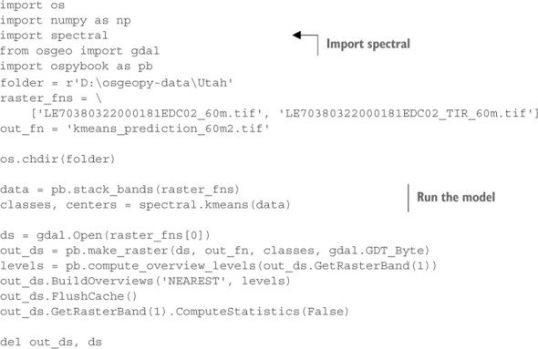
The only required parameter to the kmeans function is an array containing the predictor variables, which is in the three-dimensional array returned by stack_bands. You could also specify the number of output clusters desired, maximum number of iterations, several initial clusters, or a few other things. The default 10 clusters and 20 iterations are sufficient for the example, however. Feel free to consult the Spectral Python online documentation for more information.
Assuming you got the same results I did, the algorithm only created nine classes instead of ten, but it would have created ten if it could resolve them with the given data. I went to the trouble to try to match the resulting classes with SWReGAP classes so that you can see a visual comparison, although admittedly, this works best if you’re looking at a color version of figure 12.2. The classification is definitely different, but at least the mountains in the east are clearly separated from the flats and playas to the west. It’s possible that the match would be better if more clusters had been requested, because the SWReGAP data contains a much larger number of classes. If you were to run a classification like this, you’d have to determine what each cluster represented, as I tried to match up clusters with existing classifications.
Figure 12.2. The SWReGAP landcover dataset and one created using unsupervised classification

12.2. Supervised classification
Supervised classification, unlike unsupervised techniques, requires input from the user in the form of training data. A training dataset contains all of the independent variables that correspond to a known value for the dependent variable. For example, if you knew for a fact that a particular pixel was an agricultural field, then you could sample your input datasets, such as satellite imagery, at that location and include those pixel values as the independent variables. The model is fitted using these input data and then it can be applied to your full datasets to get a spatial representation of the model results.
It used to be that training data had to be collected by visiting locations in person and documenting first-hand what the actual classification should be. In this age of high-resolution online imagery, however, in certain cases researchers can determine these values from imagery without leaving their desks. This is definitely a more cost-effective solution, although it certainly isn’t appropriate or possible for every situation. Because accurate training datasets are essential for supervised classification, consider collecting data in the field if possible. Even if the truth can be determined by looking at imagery, the modeling process is still necessary, unless you want to manually classify every pixel.
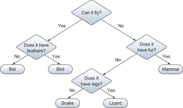
We’ll take a look at one example of supervised classification using a decision tree. This type of model consists of a hierarchical set of conditions based on the model’s independent variables, and has at least one pathway that leads to each possible outcome. Figure 12.3 shows a simple, if not accurate, example of a decision tree.
Figure 12.3. A simple example of a decision tree
Listing 12.3 uses the scikit-learn module to create a decision tree that predicts landcover type based on four bands from a Landsat 8 image and actual field data from the SWReGAP project. The locations of these ground-truthed points are shown in figure 12.4.
Figure 12.4. The locations of the ground-truthed data points used in listing 12.3

You have a text file that contains coordinates for the points in figure 12.4 and an integer value signifying the landcover class, which looks something like this:
x               y               class
377455.171684   4447157.33631   82
372685.109412   4443741.27817   119
372823.111316   4443875.28023   48
That’s a good start, but you still need the independent variables. You’ll sample the Landsat bands at the coordinates in the text file to get a dataset that looks more like this:
band1 band2 band3 band4 class
136   116   92    233   82
156   129   112   253   119
150   127   109   239   48
These data will be used to build a model that you’ll then apply to the entire extent of the Landsat bands to get a spatial dataset containing predictions. This process is shown in the following listing.
Listing 12.3. Map classification using CART


This is a little more complicated than the unsupervised example, but it’s still not that bad. The first task is to read in the coordinates and landcover class from the text file. You skip the header line, and then convert the first two values to floating-point (because they’re read in as strings) and put them in a list. When finished, this list contains a list of lists, with each inner list containing the x and y coordinates. You need the coordinates in this format later. You also put the landcover class integer in another list for later use.
Then you open one of the raster datasets so you can create a transformer object to convert between map coordinates and pixel offsets. You use this with your list of coordinates to get pixel offsets in two lists called cols and rows.
After reading the four satellite bands into a three-dimensional array, you take advantage of the fact that you can pass lists of coordinates as indices to pull data out of an array, and sample all of the points in one line of code:
sample = data[rows, cols, :]
This samples the 3D array at each of the provided row and column offsets, and returns every value in the third dimension, which is the four different satellite bands. The result is a two-dimensional array, where each row contains the four pixel values from the four bands.
Now you have all of the data required in order to fit the model, so you create a new decision tree classifier using default parameters (see the scikit-learn documentation to read the nitty-gritty details of the optional parameters) and then pass the fit method your independent variables and known landcover classifications at those same points. Make sure you don’t change the order of any of the lists; otherwise, the satellite pixel values won’t match up with the appropriate landcover value and your model won’t be fitted correctly.
clf = tree.DecisionTreeClassifier(max_depth=5)
clf = clf.fit(sample, classes)
All that’s left is to apply your fitted model to the full set of pixel values. Unfortunately, the predictor variables need to be in a two-dimensional array for this to work, so you reshape the array so that it has a large number of rows (rows * cols) and four columns, one for each band. You pass this to the predict function, and then reshape the resulting one-dimensional array back into two dimensions:
rows, cols, bands = data.shape
data2d = np.reshape(data, (rows * cols, bands))
prediction = clf.predict(data2d)
prediction = np.reshape(prediction, (rows, cols))
Another way to handle the prediction is to loop through the rows and process one at a time. An added advantage to this method is that it uses less memory. For example, my laptop crashed when I tried to run the prediction on the entire 30-meter dataset at once, but it did it row by row without a problem. You’d do it something like this:
prediction = np.empty(data.shape[0:2])
for i in range(data.shape[0]):
    prediction[i,:] = clf.predict(data[i,:,:])
Landsat bands have 0 values around the edges of the image, but those pixels are still assigned a value with the model. If all four Landsat bands contain 0 at a location, then you know that there’s no data for that cell, so you change those to 0 in the prediction data as well. You could have used any number that wasn’t a valid landcover classification, as long as you set it as the NoData value. After saving the prediction as a GeoTIFF, you copy the color table from the real SWReGAP landcover classification so you can visually compare the results. Again, you can see in figure 12.5 that this model predicts some of the same general patterns, but the results are still different. If you’re viewing this in color, you’ll see that it even failed to predict water correctly! This is a strong indication that the model needs more work. A better set of training data or independent variables would probably help.
Figure 12.5. The SWReGAP landcover dataset and one created using a decision tree

12.2.1. Accuracy assessments
Accuracy assessments are usually performed on models such as this to get an idea of how good they are. Because the model should do a good job of predicting the values that were used to build it, accuracy assessments are usually performed using a separate set of data to test the model on different values. I’ve provided a separate dataset for this, but if you need to split your data into training and assessment groups, you may want to look into the cross-validation tools in scikit-learn. One easy accuracy assessment method is to use a confusion matrix, which breaks out the results by predicted and observed values so you can see how well each classification was predicted. Although you can figure out the total percentage of correct classifications from the confusion matrix, better measures of accuracy exist. One of these is Cohen’s kappa coefficient, which ranges from -1 to 1, where the higher the number, the better the predictions. The following listing shows you how to use the scikit-learn module to construct a confusion matrix and SciKit-Learn Laboratory to compute the kappa statistic.
Listing 12.4. Confusion matrix and kappa statistic


Most of this code should look familiar because obtaining the data points needed for the accuracy assessment is similar to collecting the model training data. The difference is that instead of sampling the satellite imagery, you sample the prediction output and compare those results to the known classifications.
Once you have the known and predicted values for each location, computing kappa is easy. All you need to do is pass an array containing the true values and one containing the predicted values to the kappa function. Again, the order of the values is important, because your results will be extremely inaccurate if the known values are compared to predicted values from other locations. The kappa statistic for this model is 0.24, so the classification is slightly better than random, but it’s certainly nothing to brag about, either. In fact, a number that low indicates a poor classification.
Technically, you only need the same inputs that you use for the kappa statistic to create the confusion matrix, but you also create a list of unique classification values to use as labels. The classes will be listed in this order in the resulting matrix. After creating the matrix, you add the labels in much the same way as you added labels to your two-way histogram earlier. The matrix looks something like figure 12.6, where the rows correspond to predicted values and columns to known values. For example, 16 pixels that were predicted as class 22 were predicted correctly, but two were really class 5 and one was actually class 28.
Figure 12.6. The first few rows and columns of the confusion matrix for the classification tree model. Rows are predictions, and columns are actual values, so two pixels were predicted as class 22 but were class 5.

12.3. Summary
- Unsupervised classification algorithms group pixels based on how alike they are.
- Supervised classification algorithms use ground-truthed data to predict which set of conditions results in each class.