
Get Your Data into JMP
• To copy and paste data from another application, see “Copy and Paste Data”.
• To import data from another application, see “Import Data”.
• To enter data directly into a data table, see “Enter Data”
• To open a data table, double-click on the file, or use the File > Open command.
You can also import data into JMP from a database. For more information, see the Import Your Data chapter in the Using JMP book.
This chapter uses sample data tables and sample import data that is installed with JMP. To find these files, see “Using Sample Data” in the “Introducing JMP” chapter.
Copy and Paste Data
You can move data into JMP by copying and pasting from another application, such as Excel or a text file.
1. Open the VA Lung Cancer.xls file in Excel. This file is located in the Sample Import Data folder.
2. Select all of the rows and columns, including the column names. There are 12 columns and 138 rows.
3. Copy the selected data.
4. In JMP, select File > New > Data Table to create an empty table.
5. Select Edit > Paste with Column Names to paste the data and column headings.
If the data that you are pasting into JMP does not have column names, then you can use Edit > Paste.
Import Data
You can move data into JMP by importing data from another application, such as Excel, SAS, or text files. The basic steps to import data are as follows:
1. Select File > Open.
2. Navigate to your file’s location.
3. If your file is not listed in the Open Data File window, select the correct file type from the Files of type menu.
4. Click Open.
Example of Importing a Microsoft Excel File
1. Select File > Open.
2. Navigate to the Samples/Import Data folder.
3. Select Team Results.xls.
Note the rows and columns on which the data begin. The spreadsheet also contains two worksheets. In this example, you import the Ungrouped Team Results worksheet.
4. Click Open.
The spreadsheet opens in the Excel Import Wizard, where a preview of the data appears along with import options.
Text from the first row of the spreadsheet are column headings. However, you want text in row 3 of the spreadsheet to be converted to column headings.
5. Next to Column headers start on row, type 3, and press Enter. The column headings are updated in the data preview. The value for the first row of data is updated to 4.
6. Save the settings only for this worksheet:
‒ Deselect Use for all worksheets in the lower left corner of the window.
‒ Select Ungrouped Team Results in the upper right corner of the window.
7. Click Import to convert the spreadsheet as you specified.
When you import Excel files, JMP predicts whether columns headings exist, and if the column names are on row one. The copy and paste method is recommended for the following situations:
• If the column names are located in a row other than row one
• If the file does not include column names and the data does not start in row one
• If the file contains column names and the data does not start in row two
See “Copy and Paste Data” and the Import Your Data chapter in the Using JMP book for more information about importing Excel files.
Example of Importing a Text File
One way to import a text file is to let JMP assume the data’s format and place the data in a data table. This method uses settings that you can specify in Preferences. See the JMP Preferences chapter in the Using JMP book for information about setting text import preferences.
Another way to import a text file is to use a Text Preview window to see what your data table will look like after importing, and make adjustments. The following example shows you how to use Text Import Preview window.
1. Select File > Open.
2. Navigate to the Samples/Import Data folder.
3. Select Animals_line3.txt.
4. At the bottom of the Open window, select Data with Preview.
5. Click Open.
Figure 3.2 Initial Preview Window

This text file has a title on the first line, column names on the third line, and the data starts on line four. If you opened this directly in JMP, the Animals Data line would be the first column name, and all the column names and data afterward would be out of sync. The Preview window lets you adjust the settings before you open the file, and see how your adjustments affect the final data table.
6. Enter 3 in the File contains column names on line field.
7. Enter 4 in the Data starts on line field.
8. Click Next.
In the second window, you can exclude columns from the import and change the data modeling of the columns. For this example, use the default settings.
9. Click Import.
The new data table has columns named species, subject, miles, and season. The species and season columns are character data. The subject and miles columns are continuous numeric data.
Enter Data
You can enter data directly in a data table. The following example shows you how to enter data that was collected over several months into a data table.
Scenario
Table 3.1 shows the data from a study that investigated a new blood pressure medication. Each individual’s blood pressure was measured over a six-month period. Two doses (300mg and 450mg) of the medication were used, along with a control and placebo group. The data shows the average blood pressure for each group.
|
Month
|
Control
|
Placebo
|
300mg
|
450mg
|
|
March
|
165
|
163
|
166
|
168
|
|
April
|
162
|
159
|
165
|
163
|
|
May
|
164
|
158
|
161
|
153
|
|
June
|
162
|
161
|
158
|
151
|
|
July
|
166
|
158
|
160
|
148
|
|
August
|
163
|
158
|
157
|
150
|
Enter Data in a New Data Table
1. Select File > New > Data Table to create an empty data table.
A new data table has one column and no rows.
2. Select the column name and change the name to Month. See Figure 3.3
Note: To rename a column, you can also double-click the column name or select the column and press Enter.
Figure 3.3 Entering a Column Name

3. Select Rows > Add Rows.
The Add Rows window appears.
4. Since you want to add six rows, type 6.
5. Click OK. Six empty rows are added to the data table.
6. Enter the Month information by clicking in a cell and typing.
Figure 3.4 Month Column Completed

In the columns panel, look at the modeling type icon to the left of the column name. It has changed to reflect that Month is now nominal (previously it was continuous). Compare the modeling type shown for Column 1 in Figure 3.3 and for Month in Figure 3.4. This difference is important and is discussed in “View or Change Column Information”.
7. Double-click in the space on the right side of the Month column to add the Control column.
8. Change the name to Control.
9. Enter the Control data as shown in Table 3.1. Your data table now consists of six rows and two columns.
10. Continue adding columns and entering data as shown in Table 3.1 to create the final data table with six rows and five columns.
Change the Data Table Name
1. Double-click on the data table name (Untitled) in the Table Panel.
2. Type the new name (Blood Pressure).
Figure 3.5 Changing the Data Table Name

Transfer Data from Excel
You can use the JMP Add In for Excel to transfer a spreadsheet from Excel to JMP:
• a data table
• Graph Builder
• Distribution platform
• Fit Y by X platform
• Fit Model platform
• Time Series platform
• Control Chart platform
Set JMP Add In Preferences in Excel
To configure JMP Add In Preferences:
1. In Excel, select JMP > Preferences.
The JMP Preferences window appears.
Figure 3.6 JMP Add In Preferences

2. Accept the default Data Table Name (File name_Worksheet name) or type a name.
3. Select to Use the first rows as column names if the first row in the worksheet contains column headers.
4. If you selected to use the first rows a column headers, type the number of rows used.
5. Select to Transfer Hidden Rows if the worksheet contains hidden rows to be included in the JMP data table.
6. Select to Transfer Hidden Column if the worksheet contains hidden columns to be included in the JMP data table.
7. Click OK to save your preferences.
Transfer to JMP
To transfer an Excel worksheet to JMP:
1. Open the Excel file.
2. Select the worksheet to transfer.
3. Select JMP and then select the JMP destination:
‒ Data Table
‒ Graph Builder
‒ Distribution platform
‒ Fit Y by X platform
‒ Fit Model platform
‒ Time Series platform
‒ Control Chart platform
The Excel worksheet is opened as a data table in JMP and the selected platform’s launch window appears.
Work with Data Tables
This section contains the following information:
Tip: Consider setting the Autosave Time Out value in the General preferences to automatically save open data tables at the specified number of minutes. This autosave value also applies to journals, scripts, projects, and reports.
Edit Data
You can enter or change data, either a few cells at a time or for an entire column. This section contains the following information:
Change Values
To change a value, select a cell and type the change. You can also double-click a cell to edit it.
Note: Double-clicking in a cell is not the same as selecting a cell. A single click selects a cell. You can select more than one cell at the same time, and you can perform certain actions on selected cells. Double-clicking only lets you edit a cell. For more information about selecting rows, columns, and cells, see “Select, Deselect, and Find Values”.
Recode Values
Use the recoding tool to change all of the values in a column at once. For example, suppose that you are interested in comparing the sales of computer and pharmaceutical companies. Your current company labels are Computer and Pharmaceutical. You want to change them to Technical and Drug. Going through all 32 rows of data and changing all the values would be tedious, inefficient, and error-prone, especially if you had many more rows of data. Recode is a better option.
1. Select Help > Sample Data Library and open Companies.jmp.
2. Select the Type column by clicking once on the column heading.
3. Select Cols > Utilities > Recode.
4. In the New Value column of the Recode window, type Technical in the Computer row and Drug in the Pharmaceutical row.
5. Click Done and select the In Place option from the list.
Figure 3.7 Recode Window

All cells are updated automatically to the new values.
Create Patterned Data
Use the Fill options to populate a column with patterned data. The Fill options are especially useful if your data table is large, and typing in the values for each row would be cumbersome.
Example of Filling a Column with the Pattern
1. Add a new column.
2. Enter 1 in the first cell, 2 in the second cell, and 3 in the third cell.
3. Select the three cells, and right-click anywhere in the selected cells to see a menu.
4. Select Fill > Repeat sequence to end of table.
The rest of the column is filled with the sequence (1, 2, 3, 1, 2, 3, ...).
To continue a pattern instead of repeating it (1, 2, 3, 4, 5, 6, ...), select Continue sequence to end of table. This command can also be used to generate patterns like (1, 1, 1, 2, 2, 2, 3, 3, 3, ...).
The Fill options can recognize simple arithmetic and geometric sequences. For character data, the Fill options only repeat the values.
Select, Deselect, and Find Values
You can select rows, columns, or cells within a data table. For example, to create a subset of an existing data table, you must first select the parts of the table that you want to subset. Also, selecting rows can make data points stand out on a graph. Select rows and columns manually by clicking, or select rows that meet certain search criteria. This section contains the following information:
Select and Deselect Rows
|
Task
|
Action
|
|
Select rows one at a time
|
Click on the row number.
|
|
Select multiple adjacent rows
|
Click and drag on the row numbers.
or
Select the beginning row, and then hold down the Shift key and click the last row number.
|
|
Select multiple non-adjacent rows
|
Select the first row, and then hold down the Ctrl key and click the other row numbers.
|
|
Deselect rows one at a time
|
Hold down the Ctrl key and click the row numbers.
|
|
Deselect all rows
|
Click in the lower-triangular space in the top left corner of the table. See Figure 3.8.
|
Figure 3.8 Deselecting Rows

Select and Deselect Columns
|
Task
|
Action
|
|
Select columns one at a time
|
Click the column heading.
|
|
Select multiple adjacent columns
|
Click and drag across the column headings.
or
Select the beginning column, and then hold down the Shift key and click the last header.
|
|
Select multiple non-adjacent columns
|
Select the first column, and then hold down the Ctrl key and click the other column headings.
|
|
Deselect columns one at a time
|
Hold down the Ctrl key and click the column heading.
|
|
Deselect all columns
|
Click in the upper-triangular space in the top left corner of the table. See Figure 3.9.
|
Figure 3.9 Deselecting Columns

Select and Deselect Cells
|
Task
|
Action
|
|
Select cells one at a time
|
Click each cell individually.
|
|
Select multiple adjacent cells
|
Click and drag across the cells.
or
Select the beginning cell, and then hold down the Shift key and click the last cell.
|
|
Select multiple non-adjacent cells
|
Select the first cell, and then hold down the Ctrl key and click the other cells.
|
|
Deselect all cells
|
Click in the upper and lower triangular spaces in the top left corner of the table.
|
Search for Values
In a data table that has thousands or tens of thousands of rows, it can be difficult to locate a particular cell by scrolling through the table. If you are looking for specific information, use the Search feature to find it. If data is matches the search criteria, the cell is selected and the data grid scrolls to show it in the window. For example, the Companies.jmp data table contains information about a company that has total sales of $11,899. Use the Search feature to find that cell.
Example of Searching for a Value
1. Select Edit > Search > Find to launch the Search window.
2. In the Find what box, enter 11899.
3. Click Find. JMP finds the first cell that has 11,899 in it, and selects it.
If multiple cells meet the search criteria, click Find again to find the next cell that matches the search term.
You can also search for multiple rows at once, with each row matching some criteria.
Example of Select All Rows That Correspond to Medium-Sized Companies
1. Select Rows > Row Selection > Select Where to open the Select rows window.
2. In the column list box on the left, select Size Co.
3. In the text box on the right, enter medium.
4. Click OK.
Figure 3.10 Select Rows Window

JMP selects all of the rows that have Size Co equal to medium. There are seven.
View or Change Column Information
Information about a column is not limited to the data in the column. Data type, modeling type, format, and formulas can also be set.
To view or change column characteristics, double-click the column heading. Or, right-click the column heading and select Column Info. The Column Info window appears.
Figure 3.11 Column Info Window

Column Name
Enter or change the column name. No two columns can have the same column name.
Data Type
Select one of the following data types:
‒ Numeric specifies the column values as numbers.
‒ Character specifies the column values as non-numeric, such as letters or symbols.
‒ Row State specifies the column values as row states. This is an advanced topic. See The Column Info Window chapter in the Using JMP book.
Modeling Type
Modeling types define how values are used in analyses. Select one of the following modeling types:
‒ Continuous values are numeric only.
‒ Ordinal values are either numeric or character, and are ordered categories.
‒ Nominal values are either numeric or character, but not ordered.
Format
Select a format for numeric values. This option is not available for character data. Here are a few of the most common formats:
‒ Best lets JMP choose the best display format.
‒ Fixed Dec specifies the number of decimal places that appear.
‒ Date specifies the syntax for date values.
‒ Time specifies the syntax for time values.
‒ Currency specifies the type of currency and decimal points that are used for currency values.
Column Properties
Set special column properties such as formulas, notes, and value orders. See The Column Info Window chapter in the Using JMP book.
Lock
Lock a column, so that the values in the column cannot be changed.v
Calculate Values with Formulas
Use the Formula Editor to create columns that contain calculated values.
Scenario
The sample data table On-Time Arrivals.jmp reflects the percent of on-time arrivals for several airlines. The data was collected for March, June, and August of 1999.
Create the Formula
Suppose that you want to create a new column containing the average on-time percentage for each airline.
1. Add a new column.
2. Right-click the column heading of the new column and select Formula. The Formula Editor window appears.
Figure 3.12 Formula Editor
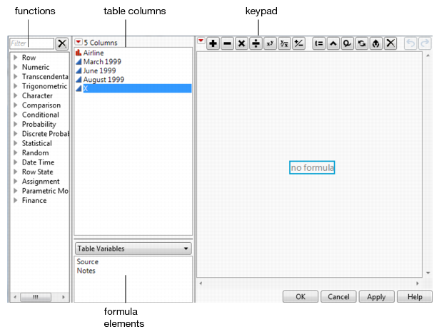
Create the formula for the average on-time percentage of each airline:
3. From the Columns list, select March 1999.
4. Click the  button on the keypad.
5. Select June 1999, followed by another sign.
6. Select August 1999.
Figure 3.13 Sum of the Months
Notice that only August 1999 is selected (has the red box around it).
7. Click on the box surrounding the entire formula.
Figure 3.14 Entire Formula Selected
8. Click the  button.
9. Type a 3 in the denominator box, and then click outside of the formula in any of the white space.
Figure 3.15 Completed Formula

10. Click OK
The new column contains the averages.
The Formula Editor has many built-in arithmetic and statistical functions. For example, another way to calculate the average on-time arrival percentage is to use the Mean function in the Statistical functions list. For details about all of the Formula Editor functions, see the Formula Editor chapter in the Using JMP book.
Filter Data
Use the Data Filter to interactively select complex subsets of data, hide these subsets in plots, or exclude them from analyses. For example, look at profit per employee for computer and pharmaceutical companies.
1. Select Help > Sample Data Library and open Companies.jmp.
2. Select Analyze > Distribution.
3. Select profit/emp and click Y, Columns.
4. Click OK.
5. From the red triangle menu for profit/emp, select Display Options > Horizontal Layout.
Figure 3.16 Distribution of profit/emp

6. Turn on Automatic Recalc by selecting Redo > Automatic Recalc from the red triangle menu for Distributions.
When this option is on, every change that you make (for example, hiding or excluding points) causes your report window to automatically update itself.
7. In the data table, select Rows > Data Filter.
8. Select Type and click Add.
9. Make sure that Select and Include are selected.
10. To filter out the Pharmaceutical companies from the Distribution results, and include only the Computer companies, click the Computer box in the Data Filter window.
The distribution results update to only include Computer companies.
Figure 3.17 Filter for Computer Companies

Conversely, to change the Distribution results to include only the Pharmaceutical companies, click the Pharmaceutical button on the Data Filter window.
Manage Data
The commands on the Tables menu (and Tabulate on the Analyze menu) summarize and manipulate data tables into the format that you need for graphing and analyzing. This section describes five of these commands:
Summary
Creates a table that contains summary statistics that describe your data.
Tabulate
Provides a drag and drop workspace to create summary statistics.
Subset
Creates a table that contains a subset of your data.
Join
Joins the data from two data tables into one new data table.
Sort
Sorts your data by one or more columns.
For complete details about these and the other Tables menu commands, see the Reshape Data chapter in the Using JMP book.
View Summary Statistics
Summary statistics, such as sums and means, can instantly provide useful information about your data. For example, if you look at the annual profit of each company out of thirty-two companies, it’s difficult to compare the profits of small, medium, and large companies. A summary shows that information immediately.
Create summary tables by using either the Summary or Tabulate commands. The Summary command creates a new data table. As with any data table, you can perform analyses and create graphs from the summary table. The Tabulate command creates a report window with a table of summary data. You can also create a table from the Tabulate report.
Summary
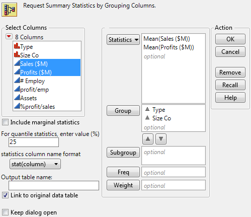
A summary table contains statistics for each level of a grouping variable. For example, look at the financial data for computer and pharmaceutical companies. Suppose that you want to calculate the mean of sales and the mean of profits, for each combination of company type and size.
1. Select Help > Sample Data Library and open Companies.jmp.
2. Select Tables > Summary.
3. Select Type and Size Co and click Group.
4. Select Sales ($M) and Profits ($M) and click Statistics > Mean.
Figure 3.18 Completed Summary Window
5. Click OK.
JMP calculates the mean of Sales ($M) and the mean of Profit ($M) for each combination of Type and Size Co.
Figure 3.19 Summary Table

The summary table contains the following:
• There are columns for each grouping variable (in this example, Type, and Size Co).
• The N Rows column shows the number of rows from the original table that correspond to each combination of grouping variables. For example, the original data table contains 14 rows corresponding to small computer companies.
• There is a column for each summary statistic requested. In this example, there is a column for the mean of Sales ($M) and a column for the mean of Profits ($M).
The summary table is linked to the source table. Selecting a row in the summary table also selects the corresponding rows in the source table.
Tabulate
Use the Tabulate command to drag columns into a workspace, creating summary statistics for each combination of grouping variables. This example shows you how to use Tabulate to create the same summary information that you just created using Summary.
1. Select Help > Sample Data Library and open Companies.jmp.
2. Select Analyze > Tabulate.
Figure 3.20 Tabulate Workspace

3. Select both Type and Size Co.
4. Drag and drop them into the Drop zone for rows.
Figure 3.21 Dragging Columns to the Row Zone

5. Right-click a heading and select Nest Grouping Columns.
The initial tabulation shows the number of rows per group.
Figure 3.22 Initial Tabulation

6. Select both Sales ($M) and Profits ($M), and drag and drop them over the N in the table.
Figure 3.23 Adding Sales and Profit

The tabulation now shows the sum of Sales ($M) and the sum of Profits ($M) per group.
Figure 3.24 Tabulation of Sums

7. The final step is to change the sums to means. Right-click Sum (either of them) and select Statistics > Mean.
Figure 3.25 Final Tabulation

The means are the same as those obtained using the Summary command. Compare Figure 3.25 to Figure 3.19.
Create Subsets
If you want to look closely at only part of your data table, you can create a subset. For example, suppose that you have already compared the sales and profits of big, medium, and small computer and pharmaceutical companies. Now you want to look at the sales and profits of only the medium-sized companies.
Creating a subset is a two-step process. First select the target data, and then extract the data into a new table.
Subset with the Subset Command
1. Select Help > Sample Data Library and open Companies.jmp.
Selecting the Rows and Columns That You Want to Subset
2. Select Rows > Row Selection > Select Where.
3. Select Size Co in the column list box on the left.
4. Enter medium in the text enter box.
5. Click OK.
6. Hold down the Ctrl key and select the Type, Sales ($M), and Profits ($M) columns.
Creating the Subset Table
7. Select Tables > Subset to launch the Subset window.
Figure 3.26 Subset Window

8. Select Selected columns to subset only the columns that you selected. You can also customize your subset table further by selecting additional options.
9. Click OK.
The resulting subset data table has seven rows and three columns. For complete details about the Subset command, see the Reshape Data chapter in the Using JMP book.
Subset with the Distribution Platform
Another way to create subsets uses the connection between platform results and data tables.
Example of Creating a Subset Using the Distribution Command
1. Select Help > Sample Data Library and open Companies.jmp.
2. Select Analyze > Distribution.
3. Select Type and click Y, Columns.
4. Click OK.
5. Double-click on the histogram bar that represents Computer to create a subset table of the Computer companies.
Caution: This method creates a linked subset table. This means if you make any changes to the data in the subset table, the corresponding value changes in the source table.
Join Data Tables
Use the Join option to combine information from multiple data tables into a single data table. For example, suppose that you have a data table containing results from an experiment on popcorn yields. In another data table, you have the results of a second experiment on popcorn yields. To compare the two experiments or to analyze the trials using both sets of results, you need to have the data in the same table. Also, the experimental data was not entered into the data tables in the same order. One of the columns has a different name, and the second experiment is incomplete. This means that you cannot copy and paste from one table into another.
Example of Joining Two Data Tables
1. Select Help > Sample Data Library and open Trial1.jmp and Little.jmp.
2. Click on Trial1.jmp to make it the active data table.
3. Select Tables > Join.
4. In the Join ‘Trial1’ With box, select Little.
5. From the Matching Specification menu, select By Matching Columns.
6. In the Source Columns boxes, select popcorn in both boxes, and then click Match.
7. In the same way, match batch and oil amt to oil in both boxes.
Your matching columns do not have to have the same name.
8. Select Include non-matches for both tables.
Since one experiment is partial, you want to include all rows, including any with missing data.
9. To avoid duplicate columns, select the Select columns for joined table option.
10. From Trial1, select all four columns and click Select.
11. From Little, select only yield and click Select.
Figure 3.27 Completed Join Window

12. Click OK.
Figure 3.28 Joined Table

Sort Tables
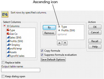
Use the Sort command to sort a data table by one or more columns in the data table. For example, look at financial data for computer and pharmaceutical companies. Suppose that you want to sort the data table by Type, then by Profits ($M). Also, you want Profits ($M) to be in descending order within each Type.
1. Select Help > Sample Data Library and open Companies.jmp.
2. Select Tables > Sort.
3. Select Type and click By to assign Type as a sorting variable.
4. Select Profits ($M) and click By.
At this point, both variables are set to be sorted in ascending order. See the ascending icon next to the variables in Figure 3.29.
Figure 3.29 Sort Ascending Icon
5. To change Profits ($M) to sort in descending order, select Profits ($M) and click the descending button.
Figure 3.30 Change Profits to Descending
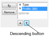
The icon next to Profits ($M) changes to descending.
6. Select the Replace Table check box.
When selected, the Replace Table option tells JMP to sort the original data table instead of creating a new table with the sorted values. This option is not available if there are any open report windows created from the original data table. Sorting a data table with open report windows might change how some of the data is displayed in the report window, especially in graphs.
7. Click OK.
The data table is now sorted by type alphabetically, and by descending profit totals within type.
..................Content has been hidden....................
You can't read the all page of ebook, please click here login for view all page.