13 Best practices for the real world

You’ve come far since the beginning of this book. You can now train image classification models, image segmentation models, models for classification or regression on vector data, time-series forecasting models, text classification models, sequence-to-sequence models, and even generative models for text and images. You’ve got all the bases covered.

However, your models so far have all been trained at a small scale—on small datasets, with a single GPU—and they generally haven’t reached the best achievable performance on each dataset we looked at. This book is, after all, an introductory book. If you are to go out in the real world and achieve state-of-the-art results on brand-new problems, there’s still a bit of a chasm that you’ll need to cross.

This penultimate chapter is about bridging that gap and giving you the best practices you’ll need as you go from machine learning student to fully fledged machine learning engineer. We’ll review essential techniques for systematically improving model performance: hyperparameter tuning and model ensembling. Then we’ll look at how you can speed up and scale up model training, with multi-GPU and TPU training, mixed precision, and leveraging remote computing resources in the cloud.

We’ll also use this chapter to show how you can access Python packages directly, even when there is no R wrapper conveniently available. This will be an essential skill as you continue in your deep learning journey. You don’t need to know Python to use Python packages from R, but if you find yourself ever reading Python documentation and asking questions like, “What are all the underscores?” head over to the appendix, Python primer for R users, which will get you up to speed as quickly as possible.

13.1 Getting the most out of your models

Blindly trying out different architecture configurations works well enough if you just need something that works okay. In this section, we’ll go beyond “works okay” to “works great and wins machine learning competitions” via a set of must-know techniques for building state-of-the-art deep learning models.

13.1.1 Hyperparameter optimization

When building a deep learning model, you have to make many seemingly arbitrary decisions: How many layers should you stack? How many units or filters should go in each layer? Should you use relu as activation, or a different function? Should you use layer_batch_normalization() after a given layer? How much dropout should you use? and so on. These architecture-level parameters are called hyperparameters to distinguish them from the parameters of a model, which are trained via backpropagation.

In practice, experienced machine learning engineers and researchers build intuition over time as to what works and what doesn’t when it comes to these choices— they develop hyperparameter-tuning skills. But no formal rules exist. If you want to get to the very limit of what can be achieved on a given task, you can’t be content with such arbitrary choices. Your initial decisions are almost always suboptimal, even if you have very good intuition. You can refine your choices by tweaking them by hand and retraining the model repeatedly—that’s what machine learning engineers and researchers spend most of their time doing. But it shouldn’t be your job as a human to fiddle with hyperparameters all day—that is better left to a machine.

Thus, you need to explore the space of possible decisions automatically, systematically, in a principled way. You need to search the architecture space and find the best-performing architectures empirically. That’s what the field of automatic hyper-parameter optimization is about: it’s an entire field of research—and an important one. The process of optimizing hyperparameters typically looks like this:

1. 1 Choose a set of hyperparameters (automatically).
2. 2 Build the corresponding model.
3. 3 Fit it to your training data, and measure performance on the validation data.
4. 4 Choose the next set of hyperparameters to try (automatically).
5. 5 Repeat.
6. 6 Eventually, measure performance on your test data.

The key to this process is the algorithm that analyzes the relationship between validation performance and various hyperparameter values to choose the next set of hyper-parameters to evaluate. Many different techniques are possible: Bayesian optimization, genetic algorithms, simple random search, and so on.

Training the weights of a model is relatively easy: you compute a loss function on a mini-batch of data and then use backpropagation to move the weights in the right direction. Updating hyperparameters, on the other hand, presents unique challenges. Consider these points:

• The hyperparameter space is typically made up of discrete decisions and, thus, isn’t continuous or differentiable. Hence, you typically can’t do gradient descent in hyperparameter space. Instead, you must rely on gradient-free optimization techniques, which naturally are far less efficient than gradient descent.
• Computing the feedback signal of this optimization process (does this set of hyperparameters lead to a high-performing model on this task?) can be extremely expensive: it requires creating and training a new model from scratch on your dataset.
• The feedback signal may be noisy: if a training run performs 0.2% better, is that because of a better model configuration, or because you got lucky with the initial weight values

Thankfully, there’s a tool that makes hyperparameter tuning simpler: KerasTuner. Let’s check it out.

USING KERASTUNER

Let’s start by installing the KerasTuner Python package:

KerasTuner lets you replace hardcoded hyperparameter values, such as units = 32, with a range of possible choices, such as Int(name = “units”, min_value = 16, max_ value = 64, step = 16). This set of choices in a given model is called the search space of the hyperparameter tuning process. To specify a search space, define a model-building function (see the next listing). It takes an hp argument, from which you can sample hyperparameter ranges, and it returns a compiled Keras model.

Listing 13.1 A KerasTuner model-building function

➊ Sample hyperparameter values from the hp object. After sampling, these values (such as the units and optimizer variables here) are just regular R constants.

➋ Different kinds of hyperparameters are available: Int, Float, Boolean, Choice.

➌ The function returns a compiled model.

If you want to adopt a more modular and configurable approach to model-building, you can also subclass the HyperModel class and define a build method, as follows.

Listing 13.2 A KerasTuner HyperModel

➊ With the object-oriented approach, we can configure model constants like num_classes to be constructor arguments.

➋ The build() method is identical to our prior build_model() standalone function, except now it is invoked by a method of a subclassed kt$HyperModel.

The next step is to define a “tuner.” Schematically, you can think of a tuner as a for loop that will repeatedly

• Pick a set of hyperparameter values
• Call the model-building function with these values to create a model
• Train the model and record its metric

KerasTuner has several built-in tuners available—RandomSearch, BayesianOptimization, and Hyperband. Let’s try BayesianOptimization, a tuner that attempts to make smart predictions for which new hyperparameter values are likely to perform best given the outcomes of previous choices:

➊ Specify the model-building function (or hypermodel instance).

➋ Specify the metric that the tuner will seek to optimize. Always specify validation metrics, because the goal of the search process is to find models that generalize.

➌ Maximum number of different model configurations ("trials") to try before ending the search.

➍ To reduce metrics variance, you can train the same model multiple times and average the results. executions_per_trial is how many training rounds (executions) to run for each model configuration (trial).

➎ Where to store search logs

➏ Whether to overwrite data in directory to start a new search. Set this to TRUE if you've modified the model-building function, or to FALSE to resume a previously started search with the same model-building function.

You can display an overview of the search space via search_space_summary():

Finally, let’s launch the search. Don’t forget to pass validation data, and make sure not to use your test set as validation data—otherwise, you’d quickly start overfitting to your test data, and you wouldn’t be able to trust your test metrics anymore:

➊ Reserve these for later.

➋ Set aside a validation set.

➌ This takes the same arguments as fit() (it simply passes them down to fit() for each new model).

➍ Make sure to pass integers where Python functions expect them, not doubles.

➎ Use a large number of epochs (you don't know in advance how many epochs each model will need), and use a callback_early_stopping() to stop training when you start overfitting.

The preceding example will run in just a few minutes, because we’re looking at only a few possible choices and we’re training on MNIST. However, with a typical search space and dataset, you’ll often find yourself letting the hyperparameter search run overnight or even over several days. If your search process crashes, you can always restart it—just specify overwrite = FALSE in the tuner so that it can resume from the trial logs stored on disk. Once the search is complete, you can query the best hyper-parameter configurations, which you can use to create high-performing models that you can then retrain.

Listing 13.3 Querying the best hyperparameter configurations

➊ Return a list of HyperParameter objects, which you can pass to the model-building function.

Usually, when retraining these models, you may want to include the validation data as part of the training data, because you won’t be making any further hyperparameter changes, and thus you will no longer be evaluating performance on the validation data. In our example, we’d train these final models on the totality of the original MNIST training data, without reserving a validation set.

Before we can train on the full training data, though, there’s one last parameter we need to settle: the optimal number of epochs to train for. Typically, you’ll want to train the new models for longer than you did during the search: using an aggressive patience value in the callback_early_stopping() saves time during the search, but it may lead to underfitting the models. Just use the validation set to find the best epoch:

➊ Note the very high patience value.

Finally, train on the full dataset for just a bit longer than this epoch count, because you’re training on more data; 20% more in this case:

Note that if you’re not worried about slightly underperforming, there’s a shortcut you can take: just use the tuner to reload the top-performing models with the best weights saved during the hyperparameter search, without retraining new models from scratch:

One important issue to think about when doing automatic hyperparameter optimization at scale is validation set overfitting. Because you’re updating hyperparameters based on a signal that is computed using your validation data, you’re effectively training them on the validation data, and thus they will quickly overfit to the validation data. Always keep this in mind.

THE ART OF CRAFTING THE RIGHT SEARCH SPACE

Overall, hyperparameter optimization is a powerful technique that is an absolute requirement for getting to state-of-the-art models on any task or to win machine learning competitions. Think about it: once upon a time, people handcrafted the features that went into shallow machine learning models. That was very much suboptimal. Now, deep learning automates the task of hierarchical feature engineering—features are learned using a feedback signal, not hand-tuned, and that’s the way it should be. In the same way, you shouldn’t handcraft your model architectures; you should optimize them in a principled way.

However, doing hyperparameter tuning is not a replacement for being familiar with model architecture best practices. Search spaces grow combinatorially with the number of choices, so it would be far too expensive to turn everything into a hyper-parameter and let the tuner sort it out. You need to be smart about designing the right search space. Hyperparameter tuning is automation, not magic: you use it to automate experiments that you would otherwise have run by hand, but you still need to handpick experiment configurations that have the potential to yield good metrics.

The good news is that by leveraging hyperparameter tuning, the configuration decisions you have to make graduate from microdecisions (what number of units do I pick for this layer?) to higher-level architecture decisions (should I use residual connections throughout this model?). And although microdecisions are specific to a certain model and a certain dataset, higher-level decisions generalize better across different tasks and datasets. For instance, pretty much every image classification problem can be solved via the same sort of search-space template.

Following this logic, KerasTuner attempts to provide premade search spaces that are relevant to broad categories of problems, such as image classification. Just add data, run the search, and get a pretty good model. You can try the hypermodels kt$applications$HyperXception and kt$applications$HyperResNet, which are effectively tunable versions of Keras Applications models.

THE FUTURE OF HYPERPARAMETER TUNING: AUTOMATED MACHINE LEARNING

Currently, most of your job as a deep learning engineer consists of munging data with R scripts and then tuning the architecture and hyperparameters of a deep network at length to get a working model, or even to get a state-of-the-art model, if you are that ambitious. Needless to say, that isn’t an optimal setup. But automation can help, and it won’t stop merely at hyperparameter tuning.

Searching over a set of possible learning rates or possible layer sizes is just the first step. We can also be far more ambitious and attempt to generate the model architecture itself from scratch, with as few constraints as possible, such as via reinforcement learning or genetic algorithms. In the future, entire end-to-end machine learning pipelines will be automatically generated, rather than handcrafted by engineer-artisans. This is called automated machine learning, or AutoML. You can already leverage libraries like AutoKeras (https://github.com/keras-team/autokeras) to solve basic machine learning problems with very little involvement on your part.

Today, AutoML is still in its early days, and it doesn’t scale to large problems. But when AutoML becomes mature enough for widespread adoption, the jobs of machine learning engineers won’t disappear—rather, engineers will move up the value-creation chain. They will begin to put much more effort into data curation, crafting complex loss functions that truly reflect business goals, as well as understanding how their models impact the digital ecosystems in which they’re deployed (such as the users who consume the model’s predictions and generate the model’s training data). These are problems that only the largest companies can afford to consider at present.

Always look at the big picture, focus on understanding the fundamentals, and keep in mind that the highly specialized tedium will eventually be automated away. See it as a gift—greater productivity for your workflows—and not as a threat to your own relevance. It shouldn’t be your job to tune knobs endlessly.

13.1.2 Model ensembling

Another powerful technique for obtaining the best possible results on a task is model ensembling. Ensembling consists of pooling the predictions of a set of different models to produce better predictions. If you look at machine learning competitions, in particular, on Kaggle, you’ll see that the winners use very large ensembles of models that inevitably beat any single model, no matter how good.

Ensembling relies on the assumption that different well-performing models trained independently are likely to be good for different reasons: each model looks at slightly different aspects of the data to make its predictions, getting part of the “truth” but not all of it. You may be familiar with the ancient parable of the blind men and the elephant: a group of blind men come across an elephant for the first time and try to understand what the elephant is by touching it. Each man touches a different part of the elephant’s body—just one part, such as the trunk or a leg. Then the men describe to each other what an elephant is: “It’s like a snake,” “Like a pillar or a tree,” and so on. The blind men are essentially machine learning models trying to understand the manifold of the training data, each from their own perspective, using their own assumptions (provided by the unique architecture of the model and the unique random weight initialization). Each of them gets part of the truth of the data, but not the whole truth. By pooling their perspectives, you can get a far more accurate description of the data. The elephant is a combination of parts: not any single blind man gets it quite right, but, interviewed together, they can tell a fairly accurate story.

Let’s use classification as an example. The easiest way to pool the predictions of a set of classifiers (to ensemble the classifiers) is to average their predictions at inference time:

➊ Use four different models to compute initial predictions.

➋ This new prediction array should be more accurate than any of the initial ones.

However, this will work only if the classifiers are more or less equally good. If one of them is significantly worse than the others, the final predictions may not be as good as the best classifier of the group.

A smarter way to ensemble classifiers is to do a weighted average, where the weights are learned on the validation data—typically, the better classifiers are given a higher weight, and the worse classifiers are given a lower weight. To search for a good set of ensembling weights, you can use random search or a simple optimization algorithm, such as the Nelder–Mead algorithm:

➊ These weights (0.5, 0.25, 0.1, 0.15) are assumed to be learned empirically.

Many possible variants exist: you can do an average of an exponential of the predictions, for instance. In general, a simple weighted average with weights optimized on the validation data provides a very strong baseline.

The key to making ensembling work is the diversity of the set of classifiers. Diversity is strength. If all the blind men only touched the elephant’s trunk, they would agree that elephants are like snakes, and they would forever stay ignorant of the truth of the elephant. Diversity is what makes ensembling work. In machine learning terms, if all of your models are biased in the same way, your ensemble will retain this same bias. If your models are biased in different ways, the biases will cancel each other out, and the ensemble will be more robust and more accurate.

For this reason, you should ensemble models that are as good as possible while being as different as possible. This typically means using very different architectures or even different brands of machine learning approaches. One thing that is largely not worth doing is ensembling the same network trained several times independently, from different random initializations. If the only difference between your models is their random initialization and the order in which they were exposed to the training data, then your ensemble will be low diversity and will provide only a tiny improvement over any single model.

One thing I have found to work well in practice—but that doesn’t generalize to every problem domain—is using an ensemble of tree-based methods (such as random forests or gradient-boosted trees) and deep neural networks. In 2014, Andrey Kolev and I took fourth place in the Higgs boson decay detection challenge on Kaggle (http://www.kaggle.com/c/higgs-boson) using an ensemble of various tree models and deep neural networks. Remarkably, one of the models in the ensemble originated from a different method than the others (it was a regularized greedy forest), and it had a significantly worse score than the others. Unsurprisingly, it was assigned a small weight in the ensemble. But to our surprise, it turned out to improve the overall ensemble by a large factor, because it was so different from every other model: it provided information that the other models didn’t have access to. That’s precisely the point of ensembling. It’s not so much about how good your best model is; it’s about the diversity of your set of candidate models.

13.2 Scaling-up model training

Recall the “loop of progress” concept we introduced in chapter 7: the quality of your ideas is a function of how many refinement cycles they’ve been through (see figure 13.1). And the speed at which you can iterate on an idea is a function of how fast you can set up an experiment, how fast you can run that experiment, and, finally, how well you can analyze the resulting data.

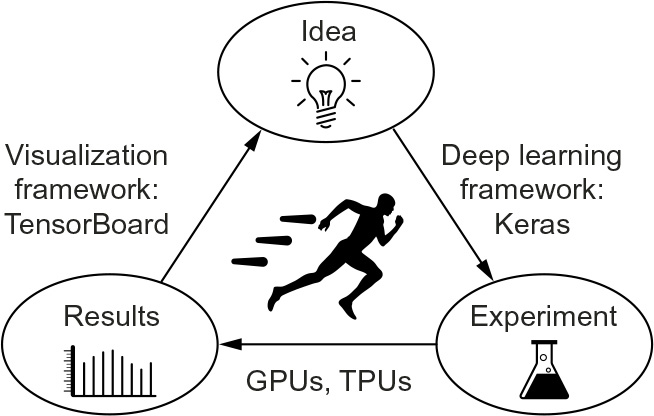
Figure 13.1 The loop of progress

As you develop your expertise with the Keras API, how fast you can code up your deep learning experiments will cease to be the bottleneck of this progress cycle. The next bottleneck will become the speed at which you can train your models. Fast training infrastructure means that you can get your results back in 10–15 minutes, and hence, you can go through dozens of iterations every day. Faster training directly improves the quality of your deep learning solutions.

In this section, you’ll learn about three ways you can train your models faster:

• Mixed-precision training, which you can use even with a single GPU
• Training on multiple GPUs
• Training on TPU

Let’s go.

13.2.1 Speeding up training on GPU with mixed precision

What if I told you there’s a simple technique you can use to speed up the training of almost any model by up to 3×, basically for free? It seems too good to but true, and yet, such a trick does exist—it’s mixed-precision training. To understand how it works, we first need to take a look at the notion of “precision” in computer science.

UNDERSTANDING FLOATING-POINT PRECISION

Precision is to numbers what resolution is to images. Because computers can process only ones and zeros, any number seen by a computer has to be encoded as a binary string. For instance, you may be familiar with uint8 integers, which are integers encoded on eight bits: 00000000 represents 0 in uint8, and 11111111 represents 255. To represent integers beyond 255, you’d need to add more bits—eight isn’t enough. Most integers are stored on 32 bits, with which you can represent signed integers ranging from –2147483648 to 2147483647.

Floating-point numbers are the same. In mathematics, real numbers form a continuous axis: there’s an infinite number of points in between any two numbers. You can always zoom in on the axis of reals. In computer science, this isn’t true: there’s a finite number of intermediate points between 3 and 4, for instance. How many? Well, it depends on the precision you’re working with—the number of bits you’re using to store a number. You can zoom up to only a certain resolution. There are three levels of precision you’d typically use:

• Half precision, or float16, where numbers are stored on 16 bits
• Single precision, or float32, where numbers are stored on 32 bits
• Double precision, or float64, where numbers are stored on 64 bit

The way to think about the resolution of floating-point numbers is in terms of the smallest distance between two arbitrary numbers that you’ll be able to safely process. In single precision, that’s around 1e-7. In double precision, that’s around 1e-16. And in half precision, it’s only 1e-3.

Almost every model you’ve seen in this book so far used single-precision numbers: it stored its state as float32 weight variables and ran its computations on float32 inputs. That’s enough precision to run the forward and backward pass of a model without losing any information—particularly when it comes to small gradient updates (recall that the typical learning rate is 1e-3, and it’s pretty common to see weight updates on the order of 1e-6).

You could also use float64, though that would be wasteful—operations like matrix multiplication or addition are much more expensive in double precision, so you’d be doing twice as much work for no clear benefits. But you could not do the same with float16 weights and computation; the gradient descent process wouldn’t run smoothly, because you couldn’t represent small gradient updates of around 1e-5 or 1e-6.

You can, however, use a hybrid approach: that’s what mixed precision is about. The idea is to leverage 16-bit computations in places where precision isn’t an issue and to work with 32-bit values in other places to maintain numerical stability. Modern GPUs and TPUs feature specialized hardware that can run 16-bit operations much faster and use less memory than equivalent 32-bits operations. By using these lower-precision operations whenever possible, you can speed up training on those devices by a significant factor. Meanwhile, by maintaining the precision-sensitive parts of the model in single precision, you can get these benefits without meaningfully impacting model quality.

A note on floating-point encoding

A counterintuitive fact about floating-point numbers is that representable numbers are not uniformly distributed. Larger numbers have lower precision: there are the same number of representable values between 2^N and 2^(N + 1) as there are between 1 and 2, for any N. That’s because floating-point numbers are encoded in three parts—the sign, the significant value (called the “mantissa”), and the exponent, in the form

<sign> * (2 ^ (<exponent> - 127)) * 1.<mantissa>

For example, the following figure shows how you would encode the closest float32 value approximating Pi.

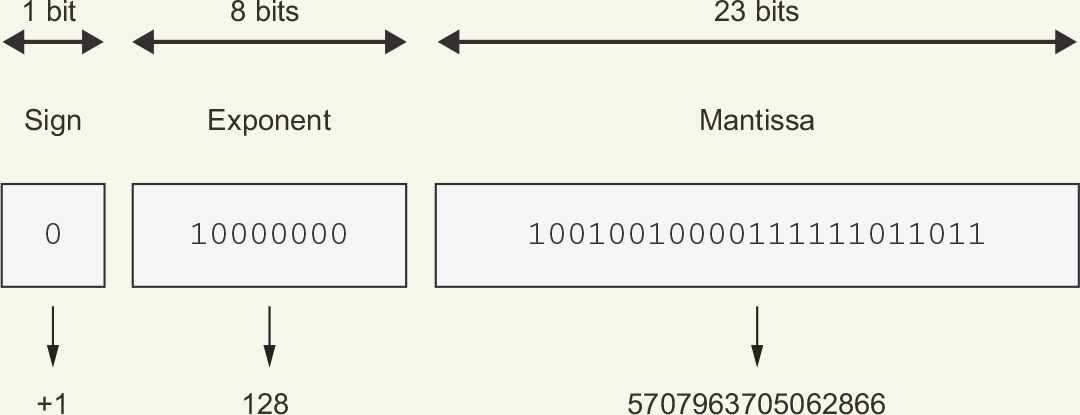
value = +1 * (2 ^ (128 - 127)) * 1.570796370562866

value = 3.1415927410125732

The number Pi encoded in single precision via a sign bit, an integer exponent, and an integer mantissa

For this reason, the numerical error incurred when converting a number to its floating-point representation can vary wildly depending on the exact value considered, and the error tends to get larger for numbers with a large absolute value.

And those benefits are considerable: on modern NVIDIA GPUs, mixed precision can speed up training by up to 3×. It’s also beneficial when training on a TPU (a subject we’ll get to in a bit), where it can speed up training by up to 60%.

MIXED-PRECISION TRAINING IN PRACTICE

When training on a GPU, you can turn on mixed precision like this:

➊ keras::keras is the Python module imported by reticulate.

Typically, most of the forward pass of the model will be done in float16 (with the exception of numerically unstable operations like softmax), whereas the weights of the model will be stored and updated in float32.

Keras layers have a variable_dtype and a compute_dtype property. By default, both of these are set to float32. When you turn on mixed precision, the compute_ dtype of most layers switches to float16, and those layers will cast their inputs to float16 and will perform their computations in float16 (using half-precision copies of the weights). However, because their variable_dtype is still float32, their weights will be able to receive accurate float32 updates from the optimizer, as opposed to half-precision updates.

Note that some operations may be numerically unstable in float16 (in particular, softmax and cross-entropy). If you need to opt out of mixed precision for a specific layer, just pass the argument dtype = “float32” to the constructor of this layer.

13.2.2 Multi-GPU training

Although GPUs are getting more powerful every year, deep learning models are getting increasingly larger, requiring ever more computational resources. Training on a single GPU puts a hard bound on how fast you can move. The solution? You could simply add more GPUs and start doing multi-GPU distributed training.

There are two ways to distribute computation across multiple devices: data parallelism and model parallelism.

With data parallelism, a single model is replicated on multiple devices or multiple machines. Each of the model replicas processes different batches of data, and then they merge their results.

With model parallelism, different parts of a single model run on different devices, processing a single batch of data together at the same time. This works best with models that have a naturally parallel architecture, such as models that feature multiple branches.

In practice, model parallelism is used only for models that are too large to fit on any single device: it isn’t used as a way to speed up training of regular models but as a way to train larger models. We won’t cover model parallelism in these pages; instead, we’ll focus on what you’ll be using most of the time: data parallelism. Let’s take a look at how it works.

GETTING YOUR HANDS ON TWO OR MORE GPUS

First, you need to get access to several GPUs. You will need to do one of two things:

• Acquire two to four GPUs, mount them on a single machine (it will require a beefy power supply), and install CUDA drivers, cuDNN, and so on. For most people, this isn’t the best option.
• Rent a multi-GPU virtual machine (VM) on Google Cloud, Azure, or AWS You’ll be able to use VM images with preinstalled drivers and software, and you’ll have very little setup overhead. This is likely the best option for anyone who isn’t training models 24/7.

We won’t cover the details of how to spin up multi-GPU cloud VMs, because such instructions would be relatively short-lived, and this information is readily available online.

SINGLE-HOST, MULTIDEVICE SYNCHRONOUS TRAINING

Once you’re able to call library(tensorflow) on a machine with multiple GPUs, you’re seconds away from training a distributed model. It works like this:

➊ Create a "distribution strategy" object. MirroredStrategy() should be your go-to solution.

➋ Use it to open a "strategy scope."

➌ Everything that creates variables should be under the strategy scope. In general, this is only model construction and compile().

➍ Train the model on all available devices.

These few lines implement the most common training setup: single-host, multidevice synchronous training, also known in TensorFlow as the “mirrored distribution strategy.” “Single host” means that the different GPUs considered are all on a single machine (as opposed to a cluster of many machines, each with its own GPU, communicating over a network). “Synchronous training” means that the state of the per-GPU model replicas stays the same at all times—there are variants of distributed training where this isn’t the case.

When you open a MirroredStrategy() scope and build your model within it, the MirroredStrategy() object will create one model copy (replica) on each available GPU. For example, if you have two GPUs, then each step of training unfolds in the following way (see figure 13.2):

1. 1 A batch of data (called the global batch) is drawn from the dataset.
2. 2 It gets split into two different sub-batches (called local batches). For instance, if the global batch has 256 samples, each of the two local batches will have 128 samples. Because you want local batches to be large enough to keep the GPU busy, the global batch size typically needs to be very large.
3. 3 Each of the two replicas processes one local batch, independently, on its own device: they run a forward pass and then a backward pass. Each replica outputs a “weight delta” describing by how much to update each weight variable in the model, given the gradient of the previous weights with respect to the loss of the model on the local batch.
4. 4 The weight deltas originating from local gradients are efficiently merged across the two replicas to obtain a global delta, which is applied to all replicas. Because this is done at the end of every step, the replicas always stay in sync: their weights are always equal.

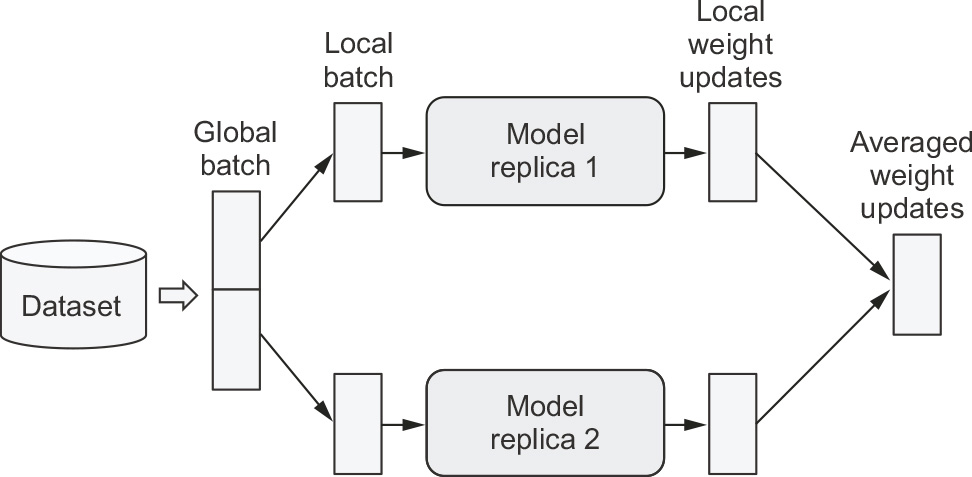
Figure 13.2 One step of MirroredStrategy training: Each model replica computes local weight updates, which are then merged and used to update the state of all replicas.

When doing distributed training, always provide your data as a TF Dataset object to guarantee best performance. (Passing your data as R arrays also works, because those are converted to TF Dataset objects by fit()). You should also make sure you leverage data prefetching: before passing the dataset to fit(), call dataset_prefetch(buffer_ size). If you aren’t sure what buffer size to pick, try leaving the default value of tf$data$AUTOTUNE, which will pick a buffer size for you.

Here’s a simple example.

Listing 13.4 Building a model in a MirroredStrategy scope

In this case, let’s train straight from R arrays in memory (which are efficiently converted to a TF Dataset by fit())—the CIFAR10 dataset:

➊ Note that multi-GPU training requires large batch sizes to make sure the device stays well utilized.

In an ideal world, training on N GPUs would result in a speedup of factor N. In practice, however, distribution introduces some overhead, in particular, merging the weight deltas originating from different devices takes some time. The effective speedup you get is a function of the number of GPUs used:

• With two GPUs, the speedup stays close to 2×.
• With four, the speedup is around 3.8×.
• With eight, it’s around 7.3×

This assumes that you’re using a large enough global batch size to keep each GPU used at full capacity. If your batch size is too small, the local batch size won’t be enough to keep your GPUs busy.

13.2.3 TPU training

Beyond just GPUs, there is a trend in the deep learning world toward moving work-flows to increasingly specialized hardware designed specifically for deep learning workflows (such single-purpose chips are known as ASICs—application-specific integrated circuits). Various companies big and small are working on new chips, but today the most prominent effort along these lines is Google’s Tensor Processing Unit (TPU), which is available on Google Cloud and via Google Colab.

Training on a TPU does involve jumping through some hoops, but it can be worth the extra work: TPUs are really, really fast. Training on a TPU V2 will typically be 15× faster than training an NVIDIA P100 GPU.

Here are some tips when using TPUs: when you’re using the GPU runtime in the cloud, your models have direct access to the GPU without you needing to do anything special. This isn’t true for the TPU runtime; there’s an extra step you need to take before you can start building a model: you need to connect to the TPU cluster. It works like this:

➊ Use TPUStrategy() just like tf$distribute$MirroredStrategy().

You don’t have to worry too much about what this does—it’s just a little incantation that connects your runtime to the device. Open sesame.

Much like in the case of multi-GPU training, using the TPU requires you to open a distribution strategy scope—in this case, a TPUStrategy() scope. TPUStrategy() fol-lows the same distribution template as MirroredStrategy()—the model is replicated once per TPU core, and the replicas are kept in sync.

Note there’s something else a bit curious about the TPU runtime: it’s a two-VM setup, meaning that the VM that hosts your notebook runtime isn’t the same VM that the TPU lives in. Because of this, you won’t be able to train from files stored on the local disk (that is, on the disk linked to the VM that hosts the instance). The TPU runtime can’t read from there. You have two options for data loading:

• Train from data that lives in the memory of the VM (not on disk). If your data is in an R array, this is what you’re already doing.
• Store the data in a Google Cloud Storage (GCS) bucket, and create a dataset that reads the data directly from the bucket, without downloading locally. The TPU runtime can read data from GCS. This is your only option for datasets that are too large to live entirely in memory

You’ll also notice that the first epoch takes a while to start. That’s because your model is getting compiled to something that the TPU can execute. Once that step is done, the training itself is blazing fast.

LEVERAGING STEP FUSING TO IMPROVE TPU UTILIZATION

Because a TPU has a lot of compute power available, you need to train with very large batches to keep the TPU cores busy. For small models, the batch size required can get extraordinarily large—upward of 10,000 samples per batch. When working with enormous batches, you should make sure to increase your optimizer learning rate accordingly; you’re going to be making fewer updates to your weights, but each update will be more accurate (because the gradients are computed using more data points), so you should move the weights by a greater magnitude with each update.

You can leverage a simple trick, however, to keep reasonably sized batches while maintaining full TPU utilization: step fusing. The idea is to run multiple steps of training during each TPU execution step. Basically, do more work in between two round trips from the VM memory to the TPU. To do this, simply specify the steps_per_execution argument in compile()—for instance, steps_per_execution = 8 to run eight steps of training during each TPU execution. For small models that are underutilizing the TPU (or GPU), this can result in a dramatic speed-up.

Summary

• You can leverage hyperparameter tuning and KerasTuner to automate the tedium out of finding the best model configuration. But be mindful of validation-set overfitting!
• An ensemble of diverse models can often significantly improve the quality of your predictions.
• You can speed up model training on GPU by turning on mixed precision— you’ll generally get a nice speed boost at virtually no cost.
• To further scale your workflows, you can use the tf$distribute$Mirrored-Strategy() API to train models on multiple GPUs.
• You can even train on Google’s TPUs by using the TPUStrategy() API. If your model is small, make sure to leverage step fusing (via the compile(…, steps_ per_execution = N) argument) to fully utilize the TPU cores.