Chapter 8: Working with Views

Introduction. 289

Views—Windows to Your Data. 289

What Views Aren’t 290

Types of Views. 291

Creating Views. 292

Displaying a View’s Contents. 293

Describing View Definitions. 294

Creating and Using Views in SAS.. 295

Views and SAS Procedures. 296

Views and DATA Steps. 297

Eliminating Redundancy. 299

Restricting Data Access—Security. 299

Hiding Logic Complexities. 300

Nesting Views. 302

Updatable Views. 304

Inserting New Rows of Data. 304

Updating Existing Rows of Data. 308

Deleting Rows of Data. 311

Deleting Views. 311

Summary. 312

In previous chapters, the examples assumed that each table had a physical existence, that is, the data stored in each table occupied storage space. In this chapter, let’s turn our attention to a different type of table structure that has no real physical existence. This structure, known as a virtual table or view, offers users and programmers an incredible amount of flexibility and control. This makes views an ideal way to look at data from a variety of perspectives and according to different users’ needs. Unlike tables, views store no data and have only a “virtual” existence. You will learn how to create, access, and delete views as you examine the many examples in this chapter.

Views are one of the more powerful features available in the SQL procedure. They are commonly referred to as “virtual tables” to distinguish them from base tables. The simple difference is that views are not tables, but instead are files that consist of executable instructions. As a query, a view appears to behave as a table with one striking difference—it does not store any data. When referenced, a view always produces up-to-date results just like a table does. So how does a view get its data? Views access data from one or more underlying tables (base tables) or other views, provide you with your own personal access to data, and can be used in DATA steps as well as by SAS procedures.

Views can be made to extend the security capabilities in dynamic environments where data duplication or data redundancy, logic complexities, and data security are an issue. When properly designed, views can be made to adhere to row-level and column-level security requirements by allowing access to only those columns and/or rows of data with relevance to the information needs of the application. Any columns and/or rows of data that are deemed “off limits,” or are classified as “restricted” can be eliminated from the view’s selection list. Consequently, views can be constructed to allow access to only those portions of an underlying table (or tables) that each user is permitted to access.

Another important feature of views is that they ensure consistently derived data by creating calculated (computed) columns that are based on some arithmetic formula (or algorithm). Database purists often design tables to be free of calculated columns, thereby relying on the view to create computed columns. By allowing views to perform data aggregation, instead of the tables themselves, processing costs can be postponed until needed or requested.

As a means of shielding users from complex logic constructs, views can be designed to look as though a database were designed specifically for a single user as well as for a group of users, each having different needs. Data references are coded once and, only when fully tested and ready for production, can be conveniently stored in common shareable libraries for all to access. Views ensure that the most current input data is used without the need for replicating partial or complete copies of the input data. They also require very little storage space because a view contains only its definition, and does not contain a copy of the data that it presents.

Views are also beneficial when queries or subqueries are repeated a number of times throughout an application. In these situations, the addition of a view enables a change to be made only once, which improves your productivity through a reduction in time and resources. The creation of view libraries should be considered so that users throughout an organization have an easily accessible array of productivity routines as they would a macro.

Views are not tables, but they are file constructs that contain compiled code that access one or more underlying tables. Because views do not physically store data, they are referred to as “virtual” tables. Unlike tables, views do not physically contain or store rows of data. Views, however, do have a physical presence and take up space. Storage demands for views are minimal because the only portion saved is the SELECT statement or query itself. Tables, on the other hand, store one or more rows of data and their attributes within their structure.

Views are created with the CREATE VIEW statement while tables are created with the CREATE TABLE statement. Because you use one or more underlying tables to create a virtual (derived) table, views provide you with a powerful method for accessing data sources.

Although views have many unique and powerful features, they also have pitfalls. First, views generally take longer to process than tables. Each time a view is referenced, the current underlying table or tables are accessed and processed. Because a view is not physically materialized until it is accessed, higher utilization costs can be expected, particularly for larger views. Also, because a view is not a data file (table) and does not contain data, an index cannot be created for a view. However, if a view is created from a data file that has a defined index, then the SQL optimizer might attempt to use the index when processing its associated WHERE clause expression. Finally, if the results of a view are used several times in the same program, it might be more efficient to save and reuse a copy of the results in a table, thereby avoiding the re-execution (materialization) of the view multiple times.

Views can be designed to achieve a number of objectives:

●         Reference a single table

●         Produce summary data across a row

●         Conceal sensitive information

●         Create updatable views

●         Grouped data based on summary functions or a HAVING clause

●         Use set operators

●         Combine two or more tables in join operations

●         Nest one view within another view

As a way to distinguish the various types of views, Joe Celko introduced a classification system that is based on the type of SELECT statement used. See SQL for Smarties: Advanced SQL Programming (Morgan Kaufman, 2014).

To help you understand the different view types, this chapter describes and illustrates view construction as well as how they can be used. A view can also have the characteristics of one or more view types, thereby being classified as a hybrid. A hybrid view, for example, could be designed to reference two or more tables, perform updates, and contain complex computations. Table 8.1 presents the different view types along with a brief description of their purpose.

Table 8.1: A Description of the Various View Types

Types of Views	Description
Single-table view	A single-table view references a single underlying (base) table. It is the most common type of view. Selected columns and rows can be displayed or hidden depending on need.
Calculated column views	A calculated column view provides summary data across a row.
Read-only view	A read-only view prevents data from being updated (as opposed to updatable views) and is used to display data only. This also serves security purposes for the concealment of sensitive information.
Updatable view	An updatable view adds (inserts), modifies, or deletes rows of data.
Grouped view	A grouped view uses query expressions that are based on a query with a GROUP BY clause.
Set operation view	A set operation view includes the union of two tables, the removal of duplicate rows, the concatenation of results, and the comparison of query results.
Joined view	A joined view is based on the joining of two or more base tables. This type of view is often used in table-lookup operations to expand (or translate) coded data into text.
Nested view	A nested view is based on one view being dependent on another view such as with subqueries.
Hybrid view	An integration of one or more view types for the purpose of handling more complex tasks.

You use the CREATE VIEW statement in the SQL procedure to create a view. When the SQL processor reads the words CREATE VIEW, it expects to find a name assigned to the newly created view. The SELECT statement defines the names assigned to the view’s columns as well as their order.

Views are often constructed so that the order of the columns is different from the base table. In the next example, a view is created with the columns appearing in a different order from the original MANUFACTURERS base table. The view’s SELECT statement does not execute during this step because its only purpose is to define the view in the CREATE VIEW statement.

SQL Code

PROC SQL;

  CREATE VIEW MANUFACTURERS_VIEW AS

    SELECT manuname, manunum, manucity, manustat

      FROM MANUFACTURERS;

QUIT;

SAS Log Results

When you create a view, you can create columns that are not present in the base table from which you built your view. That is, you can create columns that are the result of an operation (addition, subtraction, multiplication, etc.) on one or more columns in the base tables. You can also build a view using one or more unmodified columns of one or more base tables. Columns created this way are referred to as derived columns or calculated columns. In the next example, suppose that you want to create a view that consists of the product name, inventory quantity, and inventory cost from the INVENTORY base table, and a derived column of average product costs that are stored in inventory.

SQL Code

PROC SQL;

  CREATE VIEW INVENTORY_VIEW AS

    SELECT prodnum, invenqty, invencst,

           invencst/invenqty AS AverageAmount

      FROM INVENTORY;

QUIT;

SAS Log Results

You would expect the CONTENTS procedure to display information about the physical characteristics of a SAS data library and its tables. But what you might not know is that the CONTENTS procedure can also be used to display information about a view. The output that is generated from the CONTENTS procedure shows that the view contains no rows (observations) by displaying a missing value in the Observations field and a member type of VIEW. The engine used is the SQLVIEW. The following example illustrates the use of the CONTENTS procedure in the Windows environment to display the INVENTORY_VIEW view’s contents.

SQL Code

PROC CONTENTS DATA=INVENTORY_VIEW;

RUN;

Results

Because views consist of partially compiled executable statements, ordinarily you would not be able to read the code in a view definition. However, the SQL procedure provides a statement to inspect the contents of the executable instructions (stored query expression) that are contained within a view definition. Without this capability, a view’s underlying instructions (PROC SQL code) would forever remain a mystery and would make the ability to modify or customize the query expressions next to impossible. Whether your job is to maintain or customize a view, the DESCRIBE VIEW statement is the way you review the statements that make up a view. Let’s look at how a view definition is described.

The next example shows the DESCRIBE VIEW statement being used to display the INVENTORY_VIEW view’s instructions. It should be noted that results are displayed in the SAS log and not in the Output window.

SQL Code

PROC SQL;

   DESCRIBE VIEW INVENTORY_VIEW;

QUIT;

SAS Log Results

Views are accessed the same way that tables are accessed. The SQL procedure permits views to be used in SELECT queries, subsets, joins, other views, and DATA and PROC steps. Views can reference other views (as will be described in more detail in a later section of this chapter), but the referenced views must ultimately reference one or more existing base tables.

The only thing that cannot be done is to create a view from a table or view that does not already exist. When this is attempted, an error message is written in the SAS log that indicates that the view is being referenced recursively. An error occurs because the view that is being referenced directly (or indirectly) by it cannot be located or opened successfully. The next example shows the error that occurs when a view called NO_CAN_DO_VIEW is created from a non-existing view by the same name in a SELECT statement FROM clause.

SQL Code

PROC SQL;

  CREATE VIEW NO_CAN_DO_VIEW AS

    SELECT *

      FROM NO_CAN_DO_VIEW;

  SELECT *

    FROM NO_CAN_DO_VIEW;

QUIT;

SAS Log Results

In most cases but not all, views can be used just as input SAS data sets to the universe of available SAS procedures. In the first example, the INVENTORY_VIEW view is used as input to the MEANS procedure to produce simple univariate descriptive statistics for numeric variables. Accessing the INVENTORY_VIEW view is different from accessing the INVENTORY table because the view’s internal compiled executable statements are processed providing current data from the underlying table to the view itself. The view statements and the statements and options from the MEANS procedure determine what information is produced.

The next example uses the INVENTORY_VIEW view as input to the MEANS procedure to produce simple univariate descriptive statistics for numeric variables. Accessing the INVENTORY_VIEW view is different from accessing the INVENTORY table because the view derives and provides current data from the underlying table to the view itself. The view statements and the statements and options from the MEANS procedure determine what information is produced.

SAS Code

PROC MEANS DATA=INVENTORY_VIEW;

  TITLE1 ‘Inventory Statistical Report’;

  TITLE2 ‘Demonstration of a View used in PROC MEANS’;

RUN;

SAS Log Results

Results

The next example uses the INVENTORY_VIEW view as input to the PRINT procedure to produce a detailed listing of the values that are contained in the underlying base table.

Note:  It is worth noting that, as with all procedures, all procedure options and statements are available by views.

SAS Code

PROC PRINT DATA=INVENTORY_VIEW N NOOBS UNIFORM;

  TITLE1 ‘Inventory Detail Listing’;

  TITLE2 ‘Demonstration of a View used in PROC PRINT’;

  format AverageAmount dollar10.2;

RUN;

SAS Log Results

Results

As you have already seen, views can be used as input to SAS procedures as if they were data sets. You will now see that views are a versatile component that can be used in a DATA step as well. This gives you a controlled way of using views to access tables of data in custom report programs. The next example uses the INVENTORY_VIEW view as input to the DATA step as if it were a SAS base table. Notice that the KEEP= data set option reads only two of the variables from the INVENTORY_VIEW view.

SAS Code

OPTIONS FORMCHAR="|----|+|---+=|-/<>*";

DATA _NULL_;

  SET INVENTORY_VIEW (KEEP=PRODNUM AVERAGEAMOUNT);

  FILE PRINT HEADER=H1;

  PUT @10 PRODNUM

      @30 AVERAGEAMOUNT DOLLAR10.2;

RETURN;

H1: PUT @9 'Using a View in a DATA Step'

    /// @5 'Product Number'

   @26 'Average Amount';

RETURN;

RUN;

SAS Log Results

Output

Data redundancy commonly occurs when two or more users want to see the same data in different ways. To prevent redundancy, organizations should create and maintain a master database environment rather than propagate one or more subsets of data among its user communities. The latter approach creates an environment that is not only problematic for the organization but for its users and customers.

Views provide a way to eliminate or, at least, reduce the degree of data redundancy. Rather than having the same data exist in multiple forms, views create a virtual and shareable database environment for all. Problems that are related to accessing and reporting outdated information, as well as table and program change control, are eliminated.

As data security issues grow increasingly important for organizations around the globe, views offer a powerful alternative in controlling or restricting access to sensitive information. Views, like tables, can prevent unauthorized users from accessing sensitive portions of data. This is important because security breaches pose great risks not only to an organization’s data resources but to the customer as well.

Views can be constructed to show a view of data that is different from what physically exists in the underlying base tables. Specific columns can be shown while other columns are hidden. This helps prevent sensitive information such as salary, medical, or credit card data from getting into the wrong hands. Or a view can contain a WHERE clause with any degree of complexity to restrict what rows appear for a group of users while hiding other rows. In the next example, a view called SOFTWARE_PRODUCTS_VIEW is created that displays all columns from the original table except the product cost (PRODCOST) column, and restricts all rows except “Software” from the PRODUCTS table.

SQL Code

PROC SQL;

  CREATE VIEW SOFTWARE_PRODUCTS_VIEW AS

    SELECT prodnum, prodname, manunum, prodtype

      FROM PRODUCTS

        WHERE UPCASE(PRODTYPE) IN (‘SOFTWARE’);

QUIT;

SAS Log Results

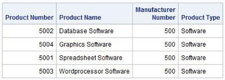
The SOFTWARE_PRODUCTS_VIEW view functions just as if it were a base table, although it contains no rows of data. All of the other columns with the exception of the product cost (PRODCOST) column are inherited from the selected columns in the PRODUCTS table. A view determines what columns and rows are processed from the underlying table and, optionally, the SELECT query that references the view can provide additional criteria during processing. In the next example, the view SOFTWARE_PRODUCTS_VIEW is referenced in a SELECT query and arranged in ascending order by product name (PRODNAME).

SQL Code

PROC SQL;

  SELECT *

    FROM SOFTWARE_PRODUCTS_VIEW

      ORDER BY prodname;

QUIT;

Results

Because complex logic constructs such as multi-way table joins, subqueries, or hard-to-understand data relationships might be beyond the skill of other staff in your area, you might want to build or customize views so that others can access the information easily. The next example illustrates how a complex query that contains a two-way join is constructed and saved as a view to simplify its use by other users.

SQL Code

PROC SQL;

  CREATE VIEW PROD_MANF_VIEW AS

    SELECT DISTINCT SUM(prodcost) FORMAT=DOLLAR10.2,

           M.manunum,

           M.manuname

      FROM PRODUCTS AS P, MANUFACTURERS AS M

        WHERE P.manunum  = M.manunum AND

              M.manuname = ‘KPL Enterprises’;

QUIT;

 

SAS Log Results

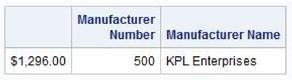
In the next example, the PROD_MANF_VIEW is simply referenced in a SELECT query. Because the view’s SELECT statement references the product cost (PRODCOST) column with a summary function but does not contain a GROUP BY clause, the note “The query requires remerging summary statistics back with the original data.” appears in the SAS log. This situation causes the sum to be calculated and then remerged with each row in the tables that are being processed.

SQL Code

PROC SQL;

  SELECT *

    FROM PROD_MANF_VIEW;

QUIT;

SAS Log Results

Results

An important feature of views is that they can be based on other views. This is called nesting. One view can access data that comes through another view. In fact, there isn’t a limit to the number of view layers that can be defined. Because of this, views can be a very convenient and flexible way for programmers to retrieve information. Although the number of views that can be nested is virtually unlimited, programmers should use care to avoid nesting views too deeply. Performance-related and maintenance-related issues can result, especially if the views are built many layers deep.

To see how views can be based on other views, two views will be created—one view that references the PRODUCTS table and the other view that references the INVOICE table. In the first example, WORKSTATION_PRODUCTS_VIEW includes only products that are related to workstations and excludes the manufacturer number. The view produces the result displayed below.

SQL Code

PROC SQL;

  CREATE VIEW WORKSTATION_PRODUCTS_VIEW AS

    SELECT PRODNUM, PRODNAME, PRODTYPE, PRODCOST

      FROM PRODUCTS

        WHERE UPCASE(PRODTYPE)=”WORKSTATION”;

QUIT;

Results

In the next example, INVOICE_1K_VIEW includes rows where the invoice price is $1,000.00 or greater and excludes the manufacturer number. When accessed from the SAS Windowing environment, the view renders the results displayed below.

SQL Code

PROC SQL;

  CREATE VIEW INVOICE_1K_VIEW AS

    SELECT INVNUM, CUSTNUM, PRODNUM, INVQTY, INVPRICE

      FROM INVOICE

        WHERE INVPRICE >= 1000.00;

QUIT;

Results

The next example illustrates how to create a view from the join of the WORKSTATION_PRODUCTS_VIEW and INVOICE_1K_VIEW views. The resulting view is nested two layers deep. When accessed from the SAS Windowing environment, the view renders the results displayed below.

SQL Code

PROC SQL;

  CREATE VIEW JOINED_VIEW AS

    SELECT V1.PRODNUM, V1.PRODNAME,

           V2.CUSTNUM, V2.INVQTY, V2.INVPRICE

      FROM WORKSTATION_PRODUCTS_VIEW  V1,

           INVOICE_1K_VIEW   V2

        WHERE V1.PRODNUM = V2.PRODNUM;

QUIT;

Results

In the next example, a third layer of view is nested to the previous view in order to find the largest invoice amount. In the next example, a view is constructed to find the largest invoice amount using the MAX summary function to compute the product of the invoice price (INVPRICE) and invoice quantity (INVQTY) from the JOINED_VIEW view.

When accessed from the SAS Windowing environment, the view produces the results displayed below.

SQL Code

PROC SQL;

  CREATE VIEW LARGEST_AMOUNT_VIEW AS

    SELECT MAX(INVPRICE*INVQTY) AS Maximum_Price

           FORMAT=DOLLAR12.2

           LABEL=”Largest Invoice Amount”

      FROM JOINED_VIEW;

QUIT;

Results

Once a view has been created from a physical table, it can then be used to modify the view’s data of a single underlying table. Essentially, when a view is updated the changes pass through the view to the underlying base table. A view that is designed in this manner is called an updatable view and can have INSERT, UPDATE, and DELETE operations performed into the single table from which it’s constructed.

Because views are dependent on getting their data from a base table and have no physical existence of their own, you should exercise care when constructing an updatable view. Although useful in modifying the rows in a table, updatable views do have a few limitations that programmers and users should be aware of.

●         An updatable view can have only a single base table associated with it. This means that the underlying table cannot be used in a join operation or with any set operators. Because an updatable view has each of its rows associated with only a single row in an underlying table, any operations that involve two or more tables will produce an error and result in update operations not being performed.

●         An updatable view cannot contain a subquery. A subquery is a complex query that consists of a SELECT statement that is contained inside another statement. This violates the rules for updatable views and is not allowed.

●         An updatable view can update a column using a view’s column alias, but cannot contain the DISTINCT keyword, have any aggregate (summary) functions, calculated columns, or derived columns associated with it. Because these columns are produced by an expression, they are not allowed.

●         An updatable view can contain a WHERE clause but cannot contain other clauses such as ORDER BY, GROUP BY, or HAVING.

In the remaining sections, three types of updatable views will be examined:

●         Views that insert one or more rows of data

●         Views that update existing rows of data

●         Views that delete one or more rows of data from a single underlying table

You can add or insert new rows of data in a view using the INSERT INTO statement. Suppose that you have a view that consists of only software products, called SOFTWARE_PRODUCTS_VIEW. The PROC SQL code that is used to create this view consists of a SELECT statement with a WHERE clause. There are four defined columns: product number, product name, product type, and product cost, in that order. When accessed from the SAS Windowing environment, the view produces the results displayed below.

SQL Code

PROC SQL;

  CREATE VIEW SOFTWARE_PRODUCTS_VIEW AS

    SELECT prodnum, prodname, prodtype, prodcost

           FORMAT=DOLLAR8.2

      FROM PRODUCTS

        WHERE UPCASE(PRODTYPE) IN (‘SOFTWARE’);

QUIT;

Results

Suppose that you want to add a new row of data to this view. This can be accomplished by specifying the corresponding values in a VALUES clause as follows.

SQL Code

PROC SQL;

  INSERT INTO SOFTWARE_PRODUCTS_VIEW

    VALUES(6002,'Security Software','Software',375.00);

QUIT;

As seen from the view results, the INSERT INTO statement added the new row of data corresponding to the WHERE logic in the view. The view contains the new row and consists of the value 6002 in product number, “Security Software” in product name, “Software” in product type, and $375.00 in product cost.

View Results

As depicted in the table results, the new row of data was added to the PRODUCTS table using the view called SOFTWARE_PRODUCTS_VIEW. The new row in the PRODUCTS table contains the value 6002 in product number, “Security Software” in product name, “Software” in product type, and $375.00 in product cost. The manufacturer number column is assigned a null value (missing value).

Table Results

Now, let’s see what happens when a row of data is added through a view that does not meet the condition(s) in the WHERE clause in the view. Suppose that you want to add a row of data that contains the value 1701 for product number, “Travel Laptop SE” in product name, “Laptop” in product type, and $4200.00 in product cost in the SOFTWARE_PRODUCTS_VIEW view.

SQL Code

PROC SQL;

  INSERT INTO SOFTWARE_PRODUCTS_VIEW

    VALUES(1701,'Travel Laptop SE','Laptop',4200.00);

QUIT;

Because the new row’s value for product type is “Laptop”, this value violates the WHERE clause condition when the view SOFTWARE_PRODUCTS_VIEW was created. As a result, the new row of data is rejected and is not added to the table PRODUCTS. The SQL procedure also prevents the new row from appearing in the view because the base table controls what the view contains.

The updatable view does exactly what it is designed to do—that is, it validate each new row of data as each row is added to the base table. Whenever the WHERE clause condition is violated, the view automatically rejects the row as invalid and restores the table to its pre-updated state by rejecting the row in error and deleting all successful inserts before the error occurred. In this example, the following error message was issued to the SAS log to confirm that the view was restored to its original state before the update took place.

 

SAS Log Results

Views will not accept new rows added to a base table when the number of columns in the VALUES clause does not match the number of columns defined in the view, unless the columns that are being inserted are specified. In the next example, a partial list of columns for a row of data is inserted with a VALUES clause. Because the inserted row of data does not contain a value for product cost, the new row will not be added to the PRODUCTS table. The resulting error message indicates that the VALUES clause has fewer columns specified than exist in the view itself, as shown in the SAS log.

SQL Code

PROC SQL;

  INSERT INTO SOFTWARE_PRODUCTS_VIEW

   VALUES(6003,'Cleanup Software','Software');

QUIT;

SAS Log Results

Suppose that a view called SOFTWARE_PRODUCTS_TAX_VIEW was created with the sole purpose of deriving each software product’s sales tax amount.

SQL Code

PROC SQL;

  CREATE VIEW SOFTWARE_PRODUCTS_TAX_VIEW AS

    SELECT prodnum, prodname, prodtype, prodcost,

           prodcost * .07 AS Tax

           FORMAT=DOLLAR8.2 LABEL=‘Sales Tax’

      FROM PRODUCTS

        WHERE UPCASE(PRODTYPE) IN (‘SOFTWARE’);

QUIT;

In the next example, an attempt is made to add a new row through the SOFTWARE_PRODUCTS_TAX_VIEW view by inserting a VALUES clause with all columns defined. The row is rejected and an error is produced because an update was attempted against a view that contains a computed (calculated) column. Although the VALUES clause contains values for all columns defined in the view, the reason the row is not inserted into the PRODUCTS table is because of the reference to a computed (or derived) column TAX (Sales Tax) as shown in the SAS log results.

SQL Code

PROC SQL;

  INSERT INTO SOFTWARE_PRODUCTS_TAX_VIEW

   VALUES(6003,'Cleanup Software','Software',375.00,26.25);

QUIT;

SAS Log Results

The SQL procedure permits rows to be updated through a view. The data manipulation language statement that is specified to modify existing data in PROC SQL is the UPDATE statement. Suppose that you want to create a view to select only laptops from the PRODUCTS table. The SQL procedure code that is used to create the view is called LAPTOP_PRODUCTS_VIEW, and it consists of a SELECT statement with a WHERE clause. There are four defined columns: product number, product name, product type, and product cost, in that specific order. When accessed, the view produces the results displayed below.

SQL Code

PROC SQL;

  CREATE VIEW LAPTOP_PRODUCTS_VIEW AS

    SELECT PRODNUM, PRODNAME, PRODTYPE, PRODCOST

      FROM PRODUCTS

        WHERE UPCASE(PRODTYPE) = 'LAPTOP';

QUIT;

Results

In the next example, all laptops are to be discounted by twenty percent and the new price is to take effect immediately. The changes that are applied through the LAPTOP_PRODUCTS_VIEW view compute the discounted product cost for “Laptop” computers in the PRODUCTS table using an UPDATE statement with corresponding SET clause.

SQL Code

PROC SQL;

  UPDATE LAPTOP_PRODUCTS_VIEW

    SET PRODCOST = PRODCOST – (PRODCOST * 0.2);

QUIT;

SAS Log Results

Results

Sometimes updates that are applied through a view can change the rows of data in the base table so that once the update is performed the rows in the base table no longer meet the criteria in the view. When this occurs, the changed rows of data cannot be displayed by the view. Essentially, the updated rows that match the conditions in the WHERE clause no longer match the conditions in the view’s WHERE clause after the updates are made. As a result, the view updates the rows with the specified changes, but it is no longer able to display the rows of data that were changed.

Suppose that you want to create a view to select laptops that cost less than $2,800.00 from the PRODUCTS table. The SQL procedure code that is used to create the view called LAPTOP_DISCOUNT_VIEW consists of a SELECT statement with a WHERE clause. There are four defined columns: product number, product name, product type, and product cost, in that order. When accessed, the view produces the results displayed below.

SQL Code

PROC SQL;

  CREATE VIEW LAPTOP_DISCOUNT_VIEW AS

    SELECT PRODNUM, PRODNAME, PRODTYPE, PRODCOST

      FROM PRODUCTS

        WHERE UPCASE(PRODTYPE) = 'LAPTOP' AND

              PRODCOST < 2800.00;

QUIT;

Results

The next example illustrates how updates are applied through a view in the Windows environment so that the rows in the table no longer meet the view’s criteria. Suppose that a fifteen percent surcharge is applied to all laptops. An UPDATE statement and SET clause are specified to allow the rows in the PRODUCTS table to be updated through the view. Once the update is performed and the view is accessed, a dialog box appears that indicates that no rows are available to display because the data from the PRODUCTS table no longer meets the view’s WHERE clause expression.

SQL Code

PROC SQL;

  UPDATE LAPTOP_DISCOUNT_VIEW

    SET PRODCOST = PRODCOST + (PRODCOST * 0.15);

QUIT;

SAS Log Results

Results

Now that you have seen how updatable views can add or modify one or more rows of data, you might have a pretty good idea how to create an updatable view that deletes one or more rows of data. Consider the following updatable view that deletes manufacturers whose manufacturer number is 600 from the underlying PRODUCTS table.

SQL Code

PROC SQL;

  DELETE FROM SOFTWARE_PRODUCTS_VIEW

    WHERE MANUNUM=600;

QUIT;

SAS Log Results

When a view is no longer needed, it’s nice to know that there is a way to remove it. Without this ability, program maintenance activities would be more difficult. To remove an unwanted view, specify the DROP VIEW statement and the name of the view. In the next example, the INVENTORY_VIEW view is deleted from the WORK library.

SQL Code

PROC SQL;

  DROP VIEW INVENTORY_VIEW;

QUIT;

 

SAS Log

 

When more than a single view needs to be deleted, the DROP VIEW statement works equally as well. Specify a comma between each view name when deleting two or more views.

SQL Code

PROC SQL;

  DROP VIEW INVENTORY_VIEW, LAPTOP_PRODUCTS_VIEW;

QUIT;

SAS Log

1.       Views are not tables and consequently do not store data (see the “Views—Windows to Your Data” section).

2.       Views access one or more underlying tables (base tables) or other views (see the “Views—Windows to Your Data” section

3.       Views improve the change control process when constructed as a “common” set of routines (see the “Views—Windows to Your Data” section).

4.       Views eliminate or reduce data redundancy (see the “Eliminating Redundancy” section).

5.       Views hide unwanted or sensitive information while displaying specific columns and/or rows (see the “Restricting Data Access—Security” section).

6.       Views shield users from making logic and/or data errors (see the “Hiding Logic Complexities” section).

7.       Nesting views too deeply can produce unnecessary confusion and maintenance difficulties (see the “Nesting Views” section).

8.       Updatable views add, modify, or delete rows of data (see the “Updatable Views” section).

9.       Views can be deleted when no longer needed (see the “Deleting Views” section).