Our objective in this chapter is to build an understanding of the theory that underpins ML and AI. In doing so, it will give us an appreciation of the education, experience and skill someone developing AI and ML systems needs to have developed.

This chapter is in no way a replacement for education at higher-level institutions and industry. If you are part of an AI or ML team, it is really important to be able to find those people who can work with the more complicated and theoretical aspects of AI. AI is a broad subject and not everyone needs to be applied mathematicians, but it is important have an appreciation that these projects can be complicated and time-consuming. So, our introduction here is designed to inspire but also to remind us that sufficient time should be given to allow members of an AI team to undertake the complex learning required for a project.

4.1 HOW WE LEARN FROM DATA

ML is widely available nowadays and it is an enabler for more involved AI as we accelerate our applications and build intelligent entities. ML is built by defining what functionality we need, writing software to implement that functionality and then constructing the machines (typically digital machines) to obtain our functionality. So, our intuitive and simple model is Functionality, Software and Hardware. AI is about learning from experience and, if we have lots of data, what type of functionality is needed to learn from those data.

4.1.1 Introductory theory of machine learning

At the core of AI is machine learning. In fact, ML is an enabler of AI. Machine learning is most often associated with the popular computation we have today, that is, digital computation. AI is about learning from experience and ML is about learning from data. We will use this as the basis of our intuitive understanding of what ML is. The most popular machines used today are digital personal computers, computer clusters and large high-performance computers. As we look forward, we will move towards optical, quantum, biological and other types of learning machines to help us.

To start, we need to think about what we are actually doing – we are going to instruct and teach a machine to help us with learning. If we use a digital machine, this means we need to understand our problem in such a way that we can let a machine, say a laptop or smartphone, do the learning for us. The hardware needs software and the software needs an algorithm and data. The algorithm will use mathematics, and we finally have our starting point.

In 2019, Gilbert Strang, a professor at the Massachusetts Institute of Technology, wrote a book on linear algebra and learning from data;⁴¹ he tells us that ML has three pillars: linear algebra, probability and statistics, and optimisation. Much earlier, in the 1990s, Graham, Knuth and Patashnik produced a textbook to help students understand the mathematics needed for computational science; we might think of it as the book that describes algorithms mathematically, how they are defined and how they are understood.⁴² These two publications are detailed, rigorous mathematical texts. Tom Mitchell’s book on machine learning, as mentioned in Chapter 1, gives a taste of the theory of ML with examples, and is again a detailed, rigorous mathematical text.²³ These books are comprehensive and not for the novice. They are relevant to mathematicians, engineers and physicists who are well versed in these types of disciplines.

AI is more than learning from data; when we think about AI products, we must also think about the world that they operate in, how actuators are controlled and how policies are decided given sensor readings and a percept. Stuart Russell and Peter Norvig’s book on AI goes into the theory and mathematics of how we frame our problem beyond just learning from data; they cover ML too. They are also very clear that AI is a universal subject, so can be applied to any intellectual task – learning from experience.⁹

What is common to these technical books on the theory of AI are some key subject areas that are worth gaining an appreciation of. These are: linear algebra, vector calculus, and probability and statistics. Linear algebra is about linear systems of equations; vector calculus is about differentiation and integration of vector spaces – or, more practically, how mathematicians, engineers and physicists describe our physical world in terms of differences and summations and probability and statistics is about the mathematics of understanding randomness.

4.1.1.1 Linear algebra

This section is designed to give an overview of linear algebra; as Gilbert Strang explains, linear algebra is the key subject to understanding data and is especially important to engineering.⁴³

We learn from data using linear algebra. In school, most of us learn about systems of equations or simultaneous equations. It is linear algebra that we use to solve equations using computers and it is at the heart of AI, ML, engineering simulation and just about every other subject that relies on digital computers.

A simple example will introduce what we mean. If we want a computer to learn, we have to represent that learning in the form of mathematical operations that a computer can undertake. It is the terrain or geometry that computers can work with. Computers can undertake these mathematical operations, such as add, subtract, divide and multiply, very quickly and accurately. Far quicker and more accurately than us humans. As we mentioned earlier, most of the problems in the real world require an adaptive or iterative approach – and computers are good at this too. In fact, they are so good at this, and quick, we might think it is easy. In doing so, we almost trivialise the amount of work that goes into preparing our machines for learning.

We will use the following set of simultaneous equations to introduce terms that we’ll need to be familiar with in linear algebra. Our learning from experience involves solving the following problem:

x + y + z = 8,

10x − 4y + 3z = 13

and

3x − 6y − z = −20,

can we find what x, y and z are?

This can be done by hand using a technique from the 1800s: Gaussian elimination. (Chinese mathematicians were aware of this technique well before Gauss⁴⁵.) We could do this by hand with a calculator, a set of log tables or an analogue computer – the slide rule; however, digital computers can do this quicker and more accurately than we can. If our problem has more unknowns, say five or even 1,000, then this would be impossible to do by hand.

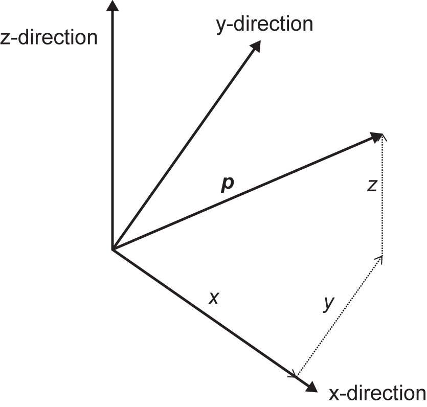
To solve this problem with a computer we need to write it in a slightly different way, so we can use linear algebra. We need to define a scalar, a vector and a matrix. This will give us the basic building blocks for our solution. A scalar is a single number that can represent a quantity. Examples are temperature, speed, time and distance. Scalars can be used to represent fields that make up a vector space. A scalar therefore is an element of a vector. An example here is a position given in terms of scalar values of direction x, y and z.

In computing, a scalar is an atomic quantity that can only hold one value. The diagram in Figure 4.1 shows a position vector, p, made up of three scalars, x, y and z. Scalars are represented as non-bold characters, for example, x, and vectors are usually bold, for example, p, or are bold and underlined, for example, p.

The example of a position vector leads to the definition of a vector. A vector has a magnitude and direction. The position vector tells us in what direction it is pointing and how far (magnitude) we have to travel in that direction. The position vector also tells us how far we need to travel in one of the directions, x, y or z. Just as a scalar is an element of a vector, a vector is an element of a vector space.

Vectors can be used to represent physical quantities such as velocity. This is very helpful in science. In AI, we can use these powerful concepts to describe learning mathematically. A simple analogy is that we map out a learning terrain and navigate it. Phrases such as steepest decent or ascent, constraints, hill-climbing or searching now have a physical analogy.

Another linear algebra term that is useful is the matrix. A matrix is an array of elements that can be numbers,

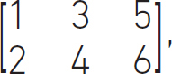
Figure 4.1 A position vector, p, made of up three scalars, x, y and z

symbols,

or expressions,

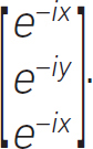
Matrices are versatile and are described by the rows and columns they have. Here, we think of matrices as two-dimensional, but these ideas can be extended to more dimensions. These are called tensors and we need these concepts for more advanced mathematics, engineering and AI. TensorFlow, the open-source software AI library, implies that our learning problems are multidimensional and involve the flow of data.

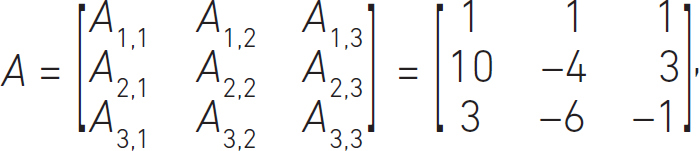
A matrix is a special form of a tensor and is made up of elements, just like scalars and vectors. The notation we use is described below. A matrix has m elements in its rows and n elements in its columns. You will come across phrases such as an m by n or m × n matrix. Each element is represented by an index; the first index is a reference to the element in the row and the second reference index is to the element in the column. It is easier to see this pictorially; a 3 by 3 (m = 3 and n = 3) matrix has elements as follows:

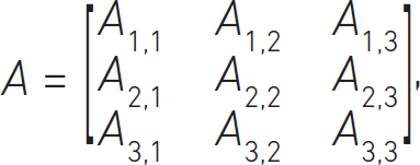
with the elements defined by indices as A_row,column. In this case, the first row is the top row and has the index 1; the second, or middle, row has index 2; and the third, or bottom, row has index 3. In mathematical texts we see matrices written as A_i,j where the index that refers to the row is i and the index that refers to the column is j. Some special matrices often used are column and row vectors. This is a 3 by 1 column vector:

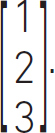
This is a 1 by 3 row vector:

[1    2    3].

So, to recap, we have scalars that are elements of a vector and vectors are elements of vector spaces. Matrices are arrays or numbers, symbols or expressions. If we go to more than two-dimensional arrays, then we call these tensors. We must be careful with tensors and matrices because using them becomes complicated.

Coming back to our system of linear equations solution using a computer, we can rewrite the problem as a matrix multiplied by a vector that equals a vector, as follows:

Ax = y,

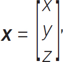
which can be written out fully as the matrix,

the column vector, x,

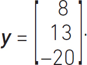
and the column vector, y,

Our solution is to find the values of x; to do this we need to find the inverse of the matrix A, which is

x = A⁻¹ y.

Computers can do this effectively and we will discuss some of the commercial and open-source software that we can use later. The answer to this problem is:

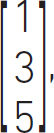
or x = 1, y = 3 and z = 5. To check this, put the values of x, y and z into each of the equations and see if you get the same answers.

Scientists, engineers and mathematicians use these techniques to set up problems with large matrices, and have to invert big matrices. This requires high-performance parallel computers, but it can be done. AI draws on these techniques also, and is another user of large supercomputers.

If we are to formulate a learning problem that we want a digital computer to solve, then we need to understand linear algebra. There are already multi-billion-dollar industries (finite element analysis, computational fluid dynamics, business analytics, etc.) using these techniques.

Armed with machines that we can use to enhance our learning, we now move onto the next core topic, that of vector calculus.

4.1.1.2 Vector calculus

Vector calculus allows us to understand vector fields using differences and summation. Or, to use the mathematical terms, differentiation and integration. A good example of a vector field is the transfer of heat. Heat can move in three directions, and we observe that it moves from hotter sources to cooler sources. So, in a simple model, we can think that the amount of heat that moves between two bodies depends on the difference in temperature. If we monitor this over a long period of time, we can add these measurements up and calculate the total amount of heat that has been transferred. This is vector calculus; it allows us to represent problems that we encounter day-to-day, from the Earth’s electromagnetic field, the movement of the oceans to the motion of vehicles on a road. When we think of a learning agent, we need to represent the state of the world. When we use the analogy of a learning problem as a terrain, then vector calculus will help us to understand how our AI is learning. In particular, how quickly it learns.

A vector is made up of scalar elements and a vector is part of a vector space. The symbol for differentiation is

and integration is

Mathematicians, scientists and engineers all work with partial and ordinary differential equations to solve their problems. Vector calculus is the cornerstone building block. If they are really lucky, there is an analytical solution to the problem; more often than not, this is not the case and they revert to numerical solutions. We are guided back towards using linear algebra.

Dorothy Vaughan used these techniques in the 1950s to help NASA land a vehicle on the moon and return it safely.⁴⁶ More generally, we don’t need to think about vector calculus applying only to space, that is, Euclidean space of x, y and z directions. The ideas and concepts can be generalised to any set of variables, and this is called multi-variable calculus. We can effectively map out a space made up of different variables and use differentiation and integration to understand what is happening.

If we were training a NN, we could map out the training time in terms of number of layers, number of nodes, bias, breadth and width of the layers, then understand how effective our training is using vector calculus. For example, we might ask what gives us the minimum error in the quickest time.

A quick example of vector calculus is useful here. Let’s imagine we want to know how much heat is being lost through the wall of our house; this is shown schematically in Figure 4.2.

Figure 4.2 Example problem for vector calculus

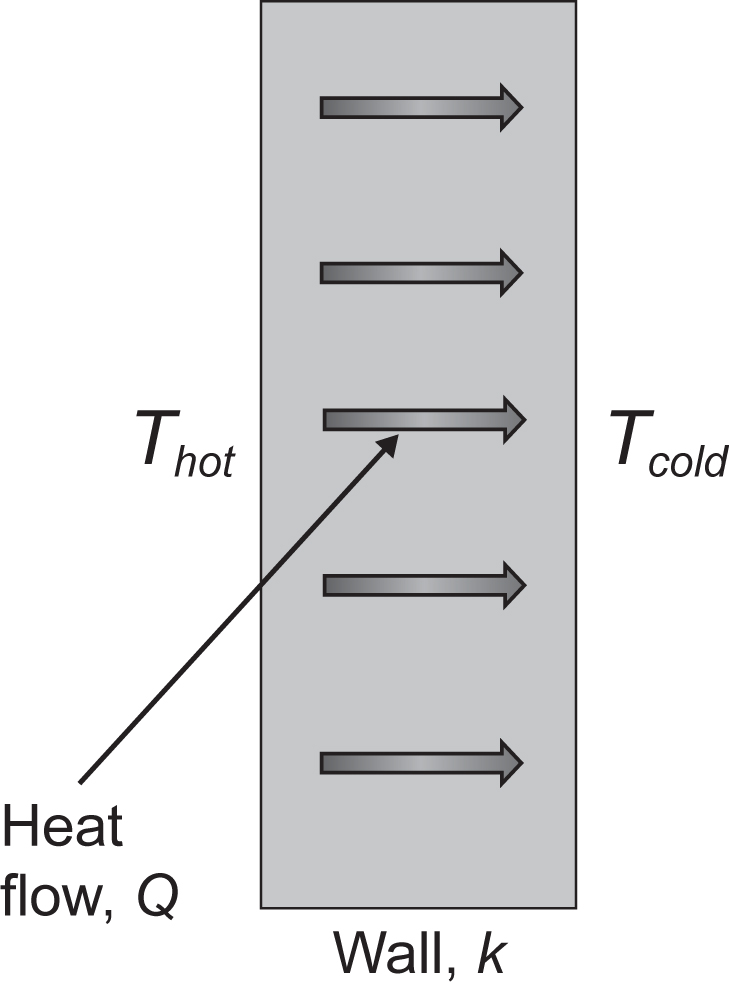
In the room in the house the temperature is hot, this is T_hot, and outside the building is the outdoor temperature, and this is cold, T_cold. We know that heat flows from hot sources to cold sources. We can also see that it is conducted through the wall. The amount of heat conducted through the wall is proportional to the thermal conductivity of the wall. The conductivity of the wall is represented as k. We would like to know how much heat we are losing through the wall; we’ll give this quantity the variable Q.

In words, the amount of heat we are losing through the wall, Q, is calculated by multiplying the thermal conductivity of the wall, k, by the temperature gradient through the wall. We also need to incorporate the surface area of the wall, A. The bigger the wall, the more heat we lose. What is the gradient? This is the temperature difference divided by the wall thickness, which is given the variable δ. Practically, this is what we are doing:

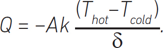
We insert the negative sign to show that heat flows from hot to cold sources and ensure we obey the second principle of thermodynamics. In vector calculus we write this as:

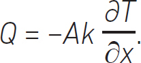
The notation is more elegant, and the derivative is written in a form called the partial differential, . This is saying that we are only interested in the gradient in the x-direction. We mentioned earlier that heat can flow in three spatial directions and, if we want a more complete picture of the heat transferred by conduction, we can rewrite our equation as:

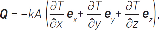
which is telling us that the heat conducted through the wall is the thermal conductivity of the wall multiplied by the gradients of temperature in each of the spatial directions. The terms e_x, e_y and e_z are unit vectors that have a magnitude of 1 and point the x, y and z directions respectively.

Vector calculus is very powerful and elegant; it also lets us express our equation in a simpler form:

Q = –Ak∇T.

What we notice here is that the heat is now a vector, Q, because we are looking at three dimensions. k and T are scalars and the operator ∇ is a vector. Our objective here is to gain an appreciation of the power and elegance of the fundamental mathematics that underpins AI. We can extend vector calculus to vector fields, not just scalar fields in our example. Applied mathematicians, physicists and engineers use these techniques daily in their jobs. When we couple vector calculus with linear algebra, we can use digital computers and machines to help us solve these equations.

Models of the state of the world (agent’s internal worlds) or ideas such as digital twinning use these techniques. These ideas work quite well on engineered systems where we have some certainty on the system we are working with. The real world, however, is not perfect and in AI we also need to deal with uncertainty or randomness. This is the next mathematical topic that AI needs – probability and statistics.

4.1.1.3 Probability and statistics

Probability and statistics are vital because the world we live in is random. The weather, traffic, stock markets, earthquakes and chance interfere with every well thought out plan. In the previous sections we introduced linear algebra and vector calculus, which are elegant subjects but also complex and need the careful attention of a domain expert. Randomness adds another dimension to the types of problem we might face with AI.

Applied mathematicians, engineers and physicists all use statistics to extend the capabilities of linear algebra and vector calculus to understand the world we live in. This is easier to observe in the diagram at Figure 4.3. Some examples are helpful here. The low-randomness, low-complexity learning is what we can work out as humans, perhaps with a calculator. For example, timetables – how long it takes for a train to travel from London to Kent. We can make these calculations easily. The low-randomness, high-complexity quadrant is learning that involves complex ideas or theory, like linear algebra or vector calculus. An example of this is how Dorothy Vaughan used computers and Fortran to calculate the re-entry of a spacecraft into Earth’s atmosphere. Low-complexity and high-randomness learning is where we can use simple ideas to understand randomness. Examples of this are games of chance, such as card games, flipping a coin or rolling dice. Physical examples are the shedding of vortices in a river as it passes around the leg of a bridge. High-complexity and high-randomness is learning that involves complex ideas that also include high randomness; examples are the weather, illness in patients, quantum mechanics, predicting the stock market. They often involve non-linearity, discontinuity and combinatorial explosions.

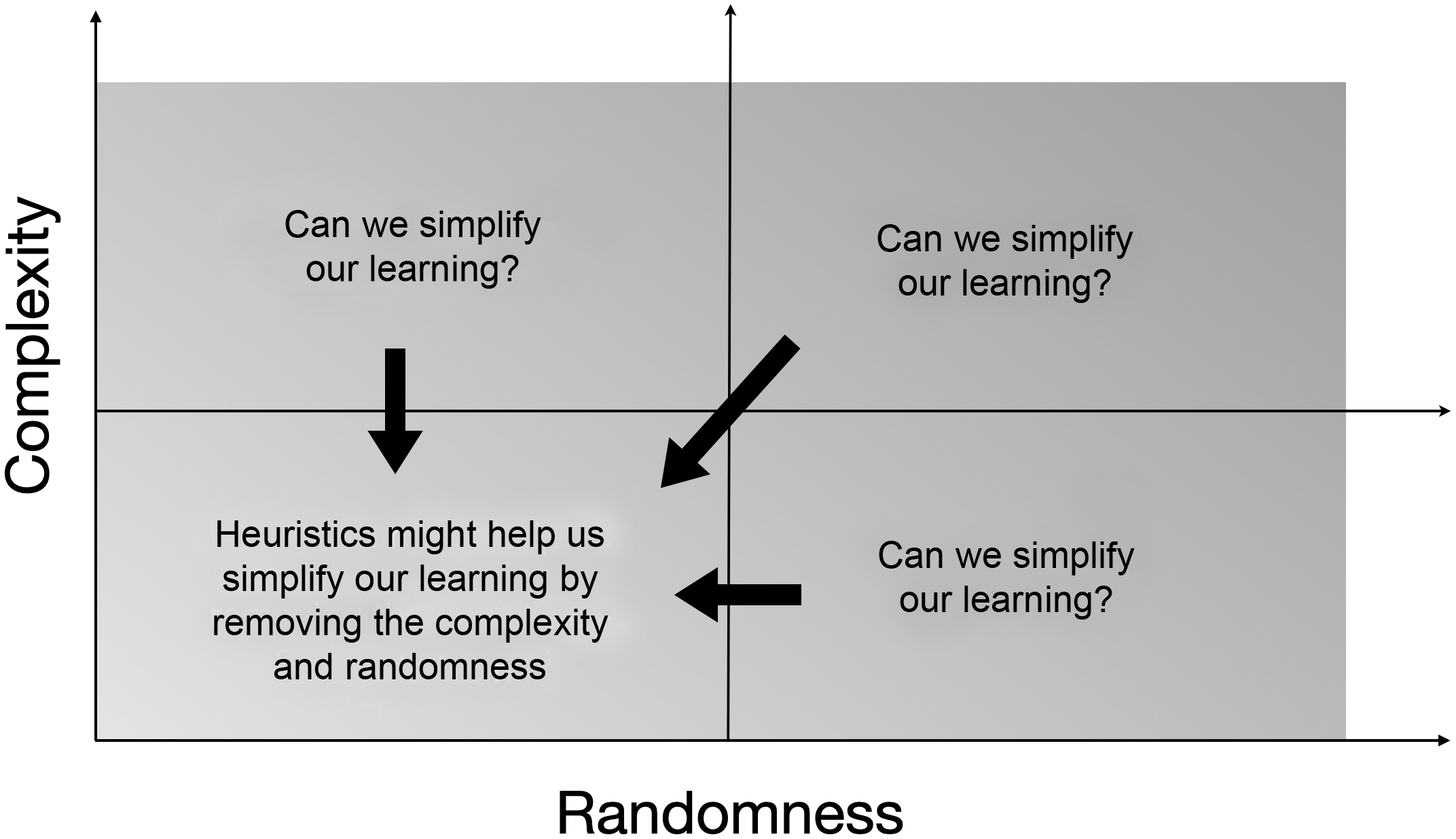
Dorothy Vaughan’s work using computers to calculate the re-entry point of a spacecraft into the Earth’s atmosphere was an elegant example of using a computer to iterate to find a solution – something that we use a lot in learning. Learning is non-linear and iterative. Dorothy took a complex problem and simplified it so a computer could guess repeatedly and find a solution. We can think of this as a heuristic that allowed a digital machine, using Fortran, to guess a solution. This is shown in Figure 4.4.

Figure 4.3 Complexity and randomness

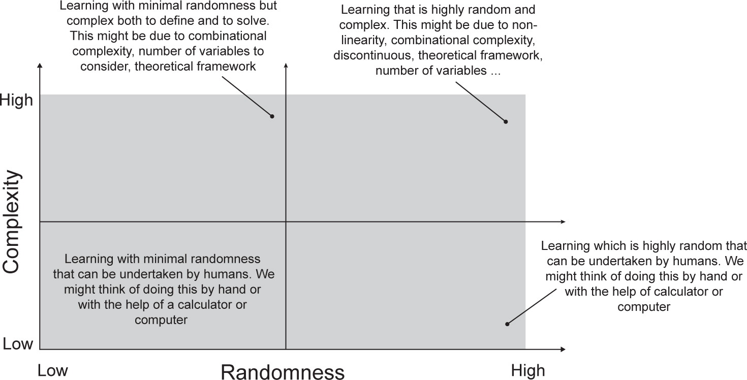
Figure 4.4 Heuristics can simplify complexity and randomness

Statistical analysis of large volumes of data is a modern-day success of digital computers. Without them we would not be able to analyse the information encoded in our genetics. Business analysts are making our activities more effective and efficient, leading to better supply chains that are integrated. An intuitive understanding of statistics and probability will help those working in AI. In AI, of particular importance, is inference and the ability to infer something about data. This started some time ago with Reverend Thomas Bayes. He came up with a theory (Bayes’ theorem) that allowed us to infer the probability or likelihood of an event happening given knowledge of factors that contribute to the event.⁴⁷ We need to remind ourselves that the factors may or may not cause the event, but we have noticed that, if they occur, it could also mean that the event will happen. For example, it rains when there are clouds in the sky (50 per cent of the time), the temperature is 19°C (33 per cent of the time), the pressure is ambient (22 per cent of the time) and so on. We can now ask ourselves what would be the probability of it raining if there are no clouds in the sky and the temperature is 19°C. Can we infer this from the data we have already?

To understand Bayes’ theorem we need to go back to basics and start with Russian mathematician, Andrey Nikolayevich Kolmogorov.⁴⁸ Kolmogorov’s contribution to probability and applied mathematics is astonishing. He wrote the three axioms of statistics. To understand them, and the theories that underpin them, we will use Venn diagrams, a pictorial way to represent statistics.⁴⁹

Say we are interested in a sample space, S, of events, A_i. The space is defined as the union of all the events:

which is a set of all possible outcomes. We need to be able to define what happens if an event never happens (is impossible), or if an event always happens (is certain) or, finally, is random (sometimes occurs). From this space of events, we would like to able to understand how these events are related to and depend on each other. To do this, Kolmogorov states that in order to define the probability of an event, Ai, occurring we need three axioms.

The first axiom is:

0 ≤ P(A_i) ≤ 1,

which defines that the probability of an event, A_i, happening lies between zero and one. If it is impossible, then it is false and has zero probability. If it is certain to occur, then it is true and has a probability of one.

The second axiom is:

P(S) = 1,

which means that the union of the sets is always equal to 1. So, if P(A) is true then P(A) = 1 and if P(A) is false then P(A) = 0. Sometimes this is explained as at least one event must have a probability of one.

The third axiom is:

P(A₁ ∪ A₂) = P(A₁) + P(A₂),

where the events A₁ and A₂ are mutually exclusive. This means that if A₁ occurs then A₂ cannot occur. Or, if A₂ occurs, then A₁ cannot occur. The third axiom leads to the addition law of probability, which deals with events that are not mutually exclusive, and this is:

P(A) + P(B) − P(A ∩ B) = P(A ∪ B),

where P(A) is the probability of A, P(B) is the probability of B, P(A ∩ B) is the probability of A and B and P(A ∪ B) is the probability of A or B. We can write this out as the probability of A or B can be found by adding the probability of A, P(A), to the probability of B, P(B), and subtracting the probability of A and B, P(A ∩ B). This makes more sense when we look at Venn diagrams.

Let’s say we have a bag of letters made up of A, B, AB and BA and this bag of letters defines our sample space, S. We’d like to know what the probability is of certain events occurring. The total number of letters we have is 100, with 43 As, 36 Bs, 15 ABs and 6 BAs.

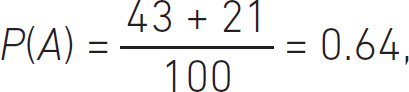
So, we can build the Venn diagram as follows. Our total space is 100 letters. We build an area of 100 units and add to it the areas of the sets for the probability of pulling an A or a B out of our bag. The probability of pulling an A out of the bag is:

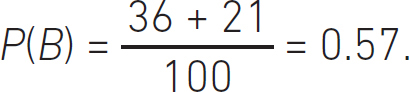
and pulling a B out of the bag is:

We have letters in our bag made up of ABs and BAs, so pulling an A or a B out of the bag is not mutually exclusive. So, just to cover the axioms, it’s worth noting that if our bag contained only Bs and no As, then the Venn diagram would look like the top diagram in Figure 4.5, and if our bag of letters contained only As, then the Venn diagram would look like the bottom diagram in the figure.

Figure 4.5 Venn diagrams for false {none of the space S is covered} and true {all of the space S is covered}

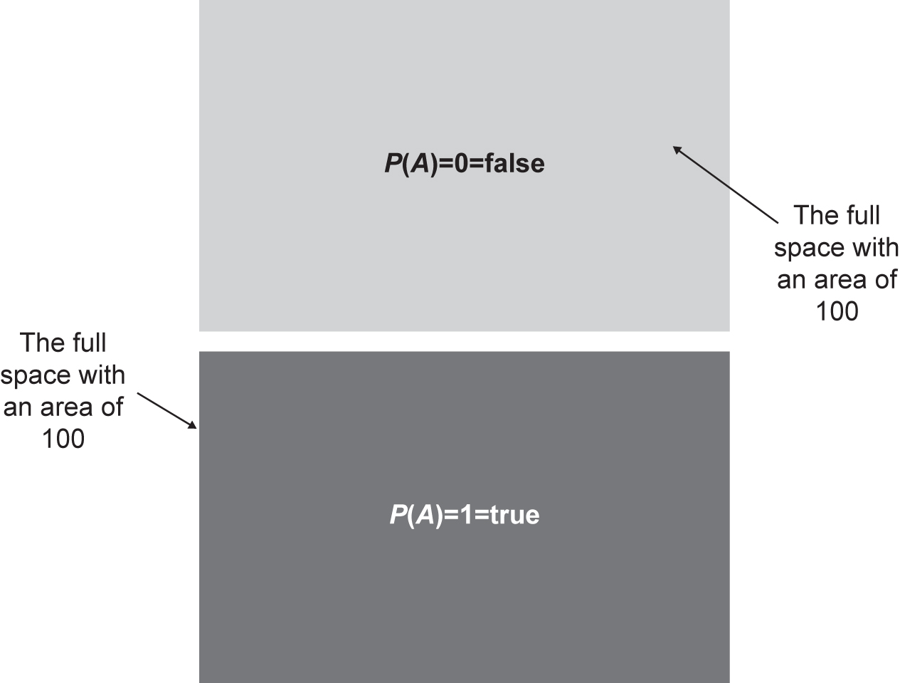
The probability of something being true is 1, and the probability of something being false is 0.

Figure 4.6 shows the Venn diagram of the probability of pulling an A (top diagram) or a B (bottom diagram) from our bag. We see that the P(A) and P(B) regions overlap. With our first look, it seems odd because, when we add up the probability, P(A) + P(B) ≠ 1. This is because we can pull out a letter of ABs or BAs, so they are not mutually exclusive. Figure 4.7 shows the probability of pulling a letter A or letter B out of our samples. We see that these regions overlap too.

Figure 4.6 Venn diagrams for the probability of finding a letter A, P(A) (top) and the probability of finding a letter B, P(B) (bottom); A and B are not mutually exclusive

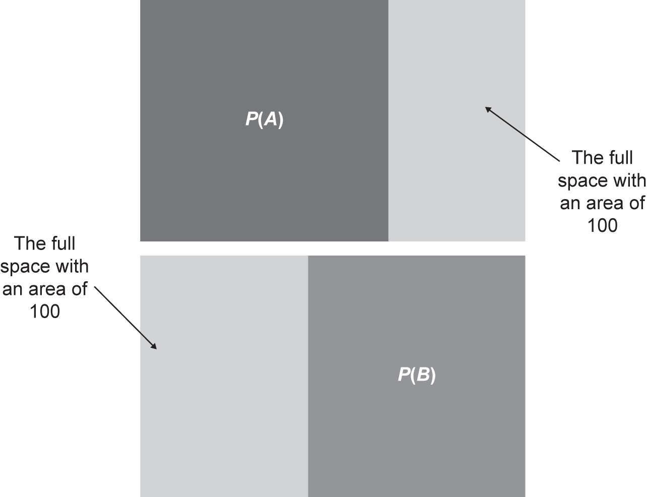
Figure 4.7 Venn diagram where A and B are not mutually exclusive. Centre region is accounted for twice in the addition law of probability

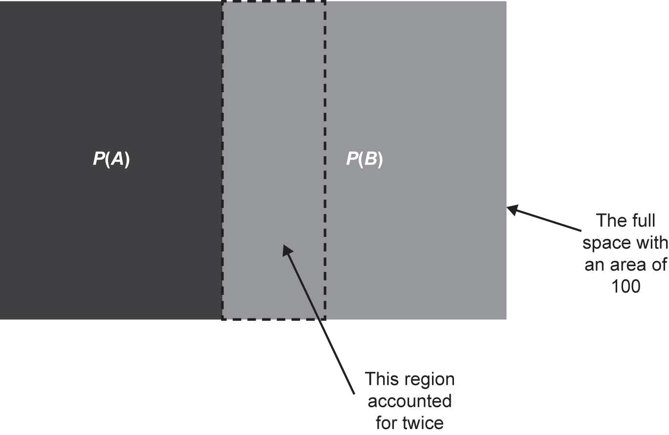
We can see why, from the addition law of probability,

P(A) + P(B) − P(A ∩ B) = P(A ∪ B).

In our bag of letters, we have letters that are ABs or BAs, so it is possible that we can obtain an A and a B. In our examples, the probability of obtaining an A and a B are:

P(A ∩ B) = 0.21,

which is the area of the overlapping region. This has been accounted for twice. The addition law of probability can be checked. If we asked the question ‘What is the probability of obtaining an A or a B?’, our answer should be 1. All of our letters are either an A or a B. Using the addition law of probability, we can check our understanding:

P(A) + P(B) − P(A ∩ B) = P(A ∪ B),

0.64 + 0.57 − 0.21 = 1.

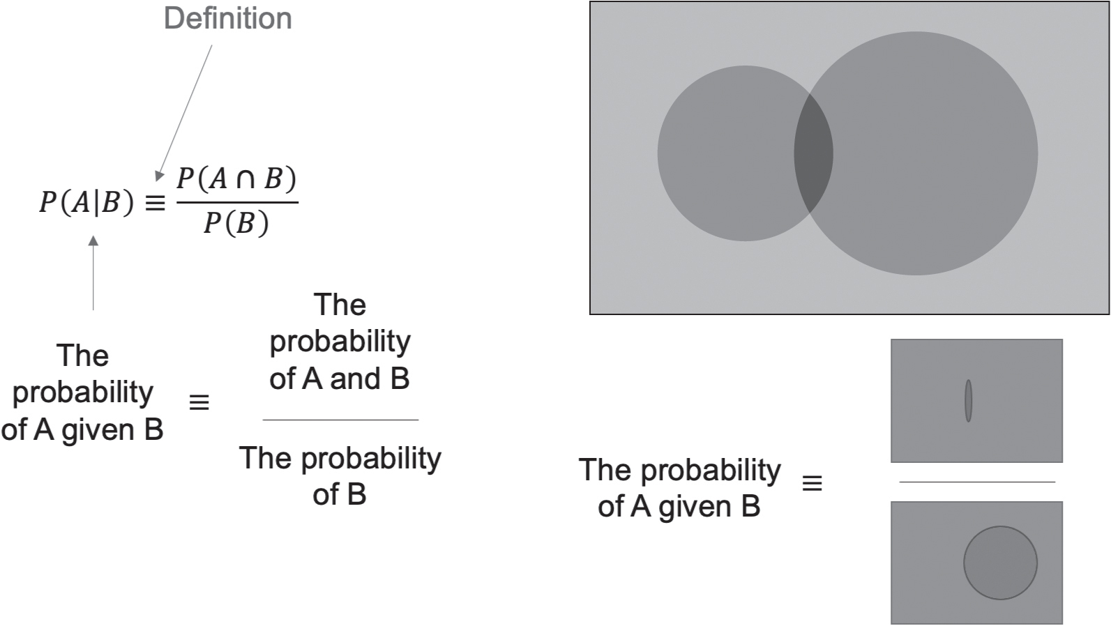
It’s also helpful to define conditional dependence, conditional independence and statistical independence. If our events occur occasionally, and are therefore random, we can ask: What is the probability of event, A, occurring if event, B, occurs? This is written as

P(A|B).

The definition of conditional probability is:

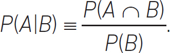
We can see what this means via the Venn diagram in Figure 4.8.

The definition of independence is:

P(A|B) ≡ P(A),

and

P(B|A) ≡ P(B),

which means that the occurrence of event A does not affect the occurrence of event B. By defining what they are, we can test if P(A) and P(B) are independent.

What this is telling us is that, on a Venn diagram, the area of P(A) is equal to the area of . Just to recap, if:

P(A|B) = P(A),

Figure 4.8 Venn diagram defining the conditional probability, P(A|B) of event A given event B. The black circle is the set of events A, and the dark grey circle is the set of events B

that is, random event, A, does not depend on the random event, B, and is therefore independent, then

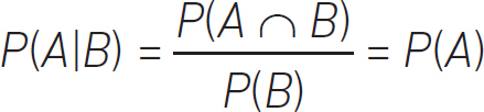
or

P(A ∩ B) = P(A)P(B).

Even though this appears intuitive in practice, when we extend this to multiple variables, it is complicated and requires careful thought. Computers are a good way to organise this.

Networks can be built using Bayes’ theorem:

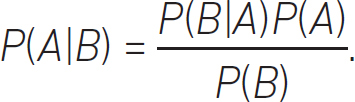
These axioms and definitions can be used to build an understanding of how random events are related to each other and to an outcome or event. This can be very useful in medical diagnosis, decision making and other areas such as the prediction of defective products or maintenance. These ML techniques involve Bayes’ theorem and the law of total probability.⁵⁰ They build networks or graphs – Bayesian networks⁵¹ – and are graphical representations of how an event is influenced by possibly known variables or causes.

In AI there are two main types of statistical learning, regression and classification.⁵² Classification tries to classify data into labels, for example name a person in a picture. Regression tries to find a relationship between variables, for example the relationship between temperature and heat transfer. This brings us nicely to how we represent random data and how we generate random numbers. Perhaps we have a limited set of statistical data and want more data points? This requires an understanding of how we represent random data.

Random data comes in two types, discrete and continuous. An example of discrete random data is the score from the roll of a dice. An example of continuous random data is the output from a pressure sensor recording the pressure on the skin of an aircraft’s wing. It is useful to know how these random data are distributed.

For discrete data we use a probability mass function, and this is shown in Figure 4.9. It is sometimes called the discrete density function. In this example we have a histogram showing the possible outcomes of rolling two dice. They are discrete values because we can only obtain the following scores from adding the two:

2, 3, 4, 5, 6, 7, 8, 9, 10, 11 and 12.

Figure 4.9 Example of a probability mass function of rolling two dice (reproduced from https://commons.wikimedia.org/wiki/File:Dice_Distribution_(bar).svg under Wikimedia Commons licence)

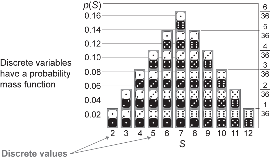
We can see that there is one way to obtain the score 2 and six ways of obtaining the score of seven. The probabilities of obtaining each score, 2 to 12, add up to 1.

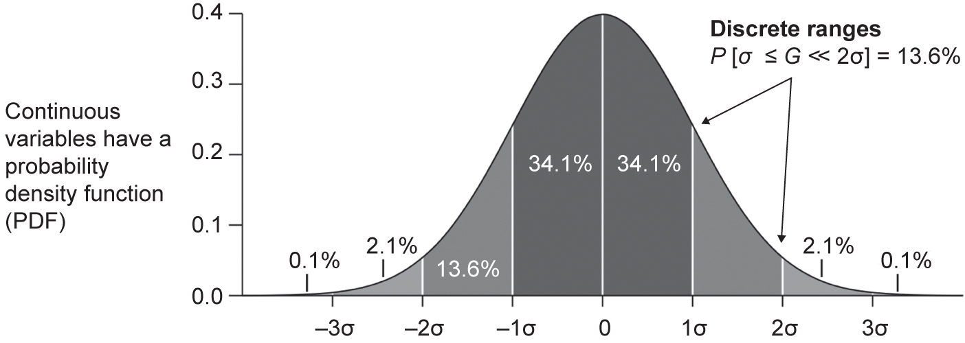
Continuous random data are represented by probability density functions (PDFs).⁵³ Probability is now thought of as being in a range, say in between two values. So, from our example of the pressure acting on the skin of an aircraft’s wing, what is the probability of the pressure being between 10Pa and 15Pa above atmosphere? Or we can think of the traditional way we grade exam scores; different ranges are associated with the grades received by the people taking the exam. This is shown in Figure 4.10. Here we see a standard Gaussian curve and the mean score is in the middle. Particular grades are associated with the bands in the curve that define a score range.

Figure 4.10 Example of a probability density function of continuous data (reproduced from https://commons.wikimedia.org/wiki/File:Standard_deviation_diagram.svg under Wikimedia Commons licence)

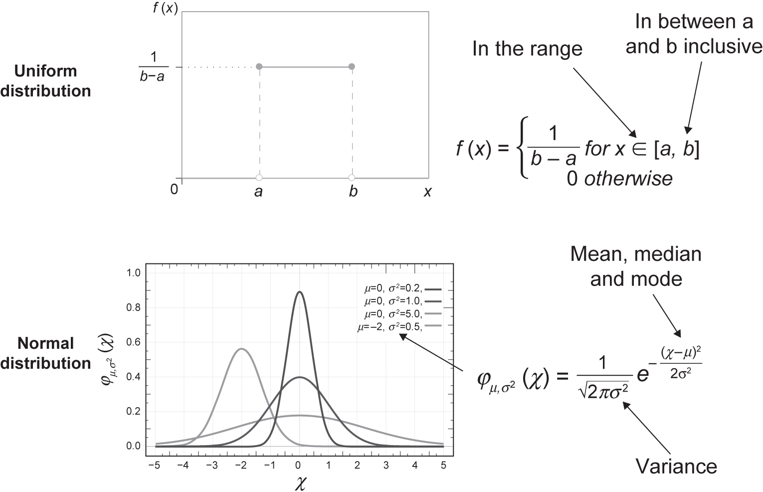
PDFs come in many forms and have different measures to describe them. A uniform and Gaussian (also called normal, Gauss, LaPlace-Gauss) PDF, along with their equations, can be seen in Figure 4.11. By describing our discrete or continuous random data via a distribution, we could also generate random numbers, and we will come back to this later. There is another important idea that can be described by example.

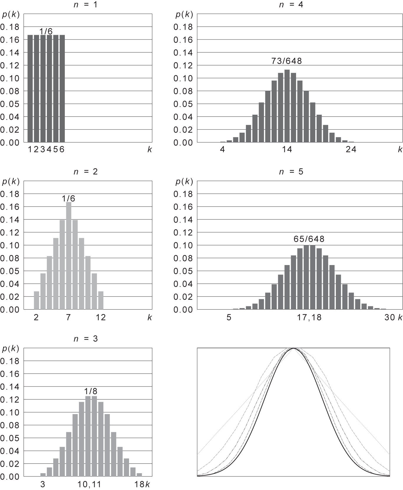
If we have five dice, and use them to generate random scores, we could ask what the distributions would look like; in particular, what happens as we increase the number of dice that contribute each set of scores we generate. This experiment is shown graphically in Figure 4.12. Rolling one die, as we expect, is a uniform distribution because each score is equally probable. When we roll two dice, the distribution is no longer uniform. As we increase the number of dice, the distribution converges onto a normal distribution. The theorem that describes this is the central limit theorem.⁵⁴ The central limit theorem suggests under certain (fairly common) conditions, the sum of many random variables will have an approximately normal distribution. So, if an event is a combination of lots of random data with different distributions, it is likely our event’s distribution will be Gaussian or normal.

From our intuitive understanding of statistics and probability we can express random data in terms of distributions and how random events relate to each other. However, we are missing how we generate random numbers or random data. Computers are explicit, linear, precise and deterministic. Fortunately, they can produce pseudo-random numbers, and the algorithms to do this are already written.^{44, 55} If we have incomplete data, but can somehow determine the probability distribution from the data we have, then we can generate random numbers with the same distribution.

Section 4.1.1 has built up an intuitive understanding of the pillars of ML and AI. Domain experts in these areas are needed if you are working with AI at an algorithmic or training level, so you will more than likely need to have these people in your team. What we have tried to show in this section is the level of mathematical understanding someone implementing AI needs to have when working with AI software. A programmer just learning Python, for example, is not prepared to develop AI algorithms; however, if a programmer is confident in the material in Section 4.1.1, then some higher-level mathematical training will make their job much easier.

Figure 4.11 Uniform and Gaussian probability density functions of continuous data (reproduced from: (top) https://en.wikipedia.org/wiki/Uniform_distribution_(continuous)#/
media/File:Uniform_Distribution_PDF_SVG.svg; (bottom) https://commons.wikimedia.org/wiki/File:Normal_Distribution_PDF.svg under Wikimedia Commons licence)

The case study in this section gives an integrated example of how vector calculus, linear algebra and probability and statistics are used at a scientific level. Vector calculus allowed us to understand the fundamental phenomena mathematically; the linear algebra allowed us to build a simulation (we might think of this as a digital twin) and generate data; and probability and statistics allowed us to generate and understand the complex non-linear nature of the data we had generated. In an AI project we might not have such tight control of the data generation, as we might have data from the real world.

4.1.2 Typical tasks in the preparation of data

Preparing data is an important aspect of all work with computers, not just AI or ML. In AI, the phrase ‘learning from experience’ is paramount. There is no guaranteed, sure fire way to ensure your data preparation is right first time. You have to learn from experience and improve your data preparation with each iteration. So, when do we stop? That is something determined by the domain expert – this person sets the standard for what is fit for purpose. An Agile project style lends itself to this very well.

Figure 4.12 An example of the central limit theorem using five dice and rolling set of scores. Top left is a set of scores from rolling one die (n = 1); middle right is a set of scores from rolling five dice (n = 5) (reproduced from https://commons.wikimedia.org/wiki/File:Dice_sum_central_limit_theorem.svg under Wikimedia Commons licence)

Data preparation is affected by numerous factors and is a science in its own right; it therefore needs experience to undertake. This experience could be learned during the project or you could employ someone already experienced to do this for you.

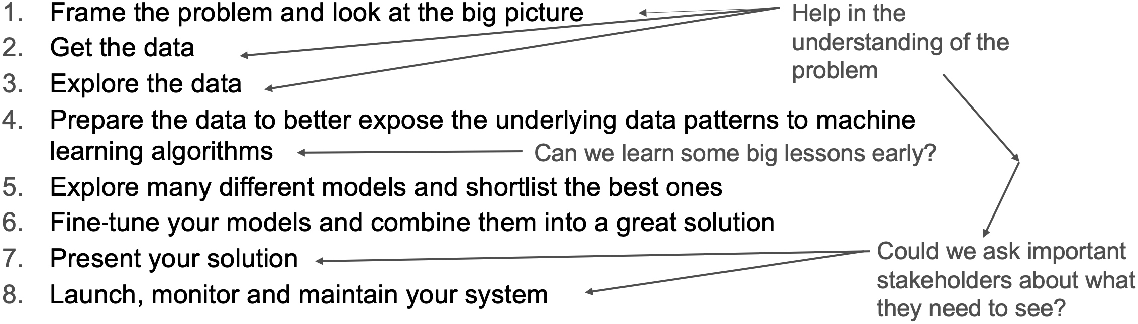
We should keep in the back of our minds that if we are working with large data sets, we have the added complexity of obtaining the data, storing them, organising them, keeping the data safe and obeying any laws associated with them – a time-consuming task in itself. Aurélien Géron’s eight stages of a machine project is a good place to start.⁵⁶ These are:

1. Frame the problem.
2. Get the data.
3. Explore the data.
4. Prepare the data to better expose the underlying data patterns to machine learning algorithms.
5. Explore many different models (or algorithms) and shortlist the best ones for the project.
6. Fine-tune your models and combine them into a great solution.
7. Present your solution.
8. Launch, monitor and maintain your system.

Again, we notice immediately that there is considerable learning from experience involved in these eight stages. They are not sequential, and we may revisit or loop over stages 1–5, 1–7 or 1–8 – going through stages 1 to 8 in one pass will be the exception rather than the rule. We might use smaller data groups so we can learn quicker because we are not processing lots of data. This can be helpful when assessing multiple algorithms as there is more work associated with this. Some learning can be gained by working on smaller subsets at an early stage. It simply reduces the time between iterations.

If we have the luxury of a large data set, we will need to break up the data into training data and test data. This is important for the trade-off, where we want to trade off complexity and error; this is covered in more detail in Section 4.1.4. We might then break up our training data into data bins of different sizes and use those different sized bins to test our algorithms. As we refine our approach, we can then use the test data to see if our learning works on data that have not been seen by the AI or ML system before.

Test data should not be used for training your AI or ML system. One of the reasons for doing this is that the algorithm will use the test data while training so we already know how well the algorithm deals with these data. It is essentially a waste of time because we are not adding further information to the system. Independent test data gives us an independent test of the ML we have done.

Once we have our data and they are divided up into appropriate bins, we can then start to clean or scrub the data. This means that we prepare our data in such a way that they give our algorithms the best chance of success.

In AI, we can encounter many types of data, such as numbers, strings, Booleans, or they could be more sophisticated data, such as audio files, movie files, script, text, documents and, perhaps, signals from actuators, sensors – we might even have to generate our own data in simulations. Digital twin is an exciting development that has gained momentum over the last 20 years or so. Data will come to us in many forms, in varying quantities.

Big Data is a term that often describes the vast array of data that can be found on the internet. Big Data has the following characteristics:⁵⁷

• Volume measures the quantity of stored and generated data.
• Variety measures the nature and type of data.
• Velocity measures the speed at which the data is moving.
• Veracity measures the data quality, value or utility.

These are self-explanatory, but the last one recognises that we may have data that are of no use or utility is of low quality. Part of the preparation of data is data cleaning or data scrubbing. As we are going through the stages of a ML project, we must always be aware of the quality of our data preparation. Poor data preparation will give spurious ML results or misrepresent the data we are trying to analyse.

Scrubbing can include:

• reducing the volume of the data we are working on, perhaps removing irrelevant data;
• reformatting data;
• removing incomplete or duplicated data;
• dealing with missing data;
• generating data;
• scaling data so algorithms perform well.

There are many tools and techniques for data preparation and standard libraries to help us, and we need experience to do this well.

As important as data preparation is data visualisation. Visualisation of data (see Section 4.1.5) will also affect how you prepare your data. This is often overlooked until we try to visualise a data set that spans multiple processors on a large supercomputer.

4.1.3 Typical types of machine learning algorithms

If we have prepared our data well and are confident they can be used to test a hypothesis, then we can begin to understand the types of algorithms we employ in ML. What we mean by ‘type’ is the broad categories that define our algorithms. They are typically organised as follows:⁹

• supervised learning – these types of algorithm use labelled (actual solution) data to train the algorithm (see Figure 4.13).
• unsupervised learning – these types of algorithm use unlabelled data to train the algorithm (see Figure 4.14).
• semi-supervised learning – these types of algorithm use labelled and unlabelled data to train the algorithm (see Figure 4.15).
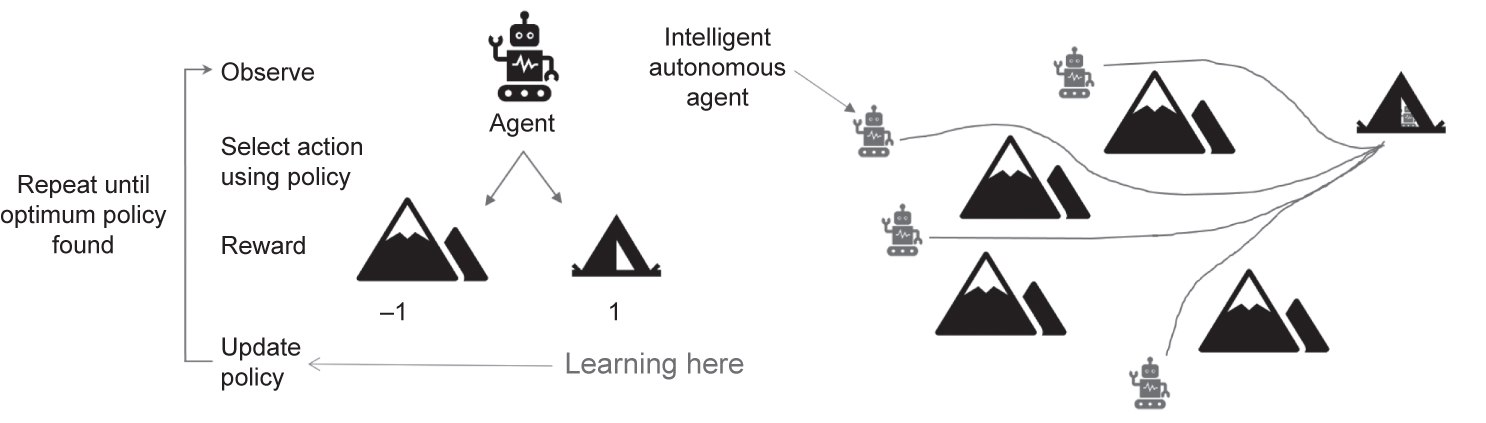
• reinforcement learning – these types of algorithm use the learning of an agent to achieve a goal that is measured in terms of a reward or penalty (see Figure 4.16).

Examples of each of the types of ML are:

• supervised learning – classification, regression (linear, logistic), support vector machines, decision forests, neural networks, neighbours;
• unsupervised learning – clustering, association rule learning, dimensionality reduction, neural networks;
• semi-supervised learning – combinations of supervised and unsupervised algorithms;
• reinforcement learning – Monte-Carlo, direct policy search, temporal difference learning.

We can also categorise the way an algorithm learns in terms of the data it is working with.

Batch learning describes learning from large data sets. All of the data are used to train and test the algorithm. The computer resources required are governed by the volume, velocity, variety and veracity of data. This learning is done offline. Online learning is undertaken with data in small or mini batches. Learning occurs as data become available – an example is a system that learns from stock market prices.

There will be times when we come across types of learning from examples or learning from examples to build a model; these types of learning are called instance-based learning and model-based learning, respectively. These are possibly the simplest form of learning.

Figure 4.13 Supervised learning

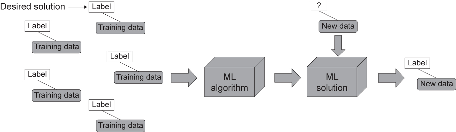
Figure 4.14 Unsupervised learning

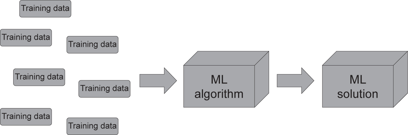
Figure 4.15 Semi-supervised learning

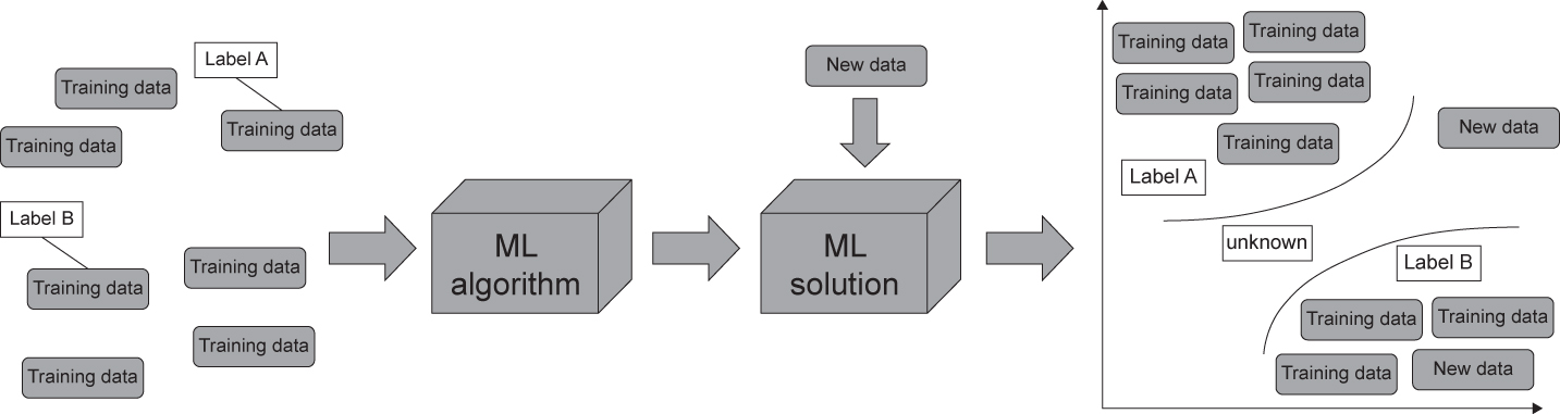
Figure 4.16 Reinforcement learning

4.1.4 Hyper-parameters, algorithms and the trade-off – under- and over-fitting

Our learning from experience involves assessing the efficacy of an algorithm to test our hypothesis. We will try different types of algorithm and adjust the algorithms’ tuning parameters to get them to perform the best they can. The tuning parameters are called hyper-parameters and they are used to set up our algorithms; or, to put it another way, they tell the algorithm how to learn. Examples of hyper-parameters include layers in a decision tree or NN, the order of a curve in regression, the number of nodes in a NN, the type of activation function, or the accuracy of a classification.

We will not know before we start what our hyper-parameters need to be to obtain the most effective algorithm. This is part of our learning from experience as we build our ML system. There are also many ways to assess the efficacy of an algorithm. The most common one used is the trade-off between complexity and accuracy. To do this, we need to understand under- and over-fitting.

These are exactly as their names imply: over-fitting the model over-fits the data too well, and under-fitting under-fits the data and does not capture the true nature of them. You can reproduce over-fitting and under-fitting on a spreadsheet by simply fitting different curves to a data set.

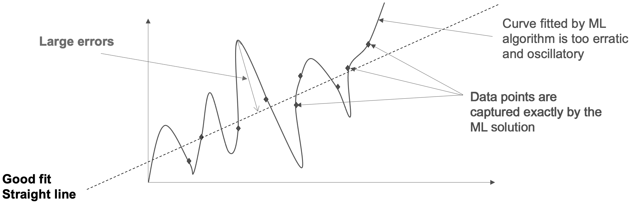
With over-fitting (see Figure 4.17) we have a data set that represents a linear straight line. This could be from experimental measures of temperature through a metal bar. The good fit straight dashed line in the graph shows the best fit to the data set. There is only a small variation of the data when compared to the best fit straight line. If we try to be too clever and use a more complex mathematical fit, say a parabola or a higher order polynomial, then we will begin to see larger errors. In the curve fitting example, the higher the order of the curve, the more oscillatory the data fit we obtain. These show up as large errors away from the actual data points we use to train our ML solution. In fact, if we have nine data points, we need a ninth order polynomial to obtain an exact match of the data points with our polynomial. However, this ninth order polynomial could oscillate widely and be a very poor fit away from the data points. To recap, over-fitting means our model or algorithm is too complicated for the data we are working with.

Figure 4.17 A simple example of over-fitting

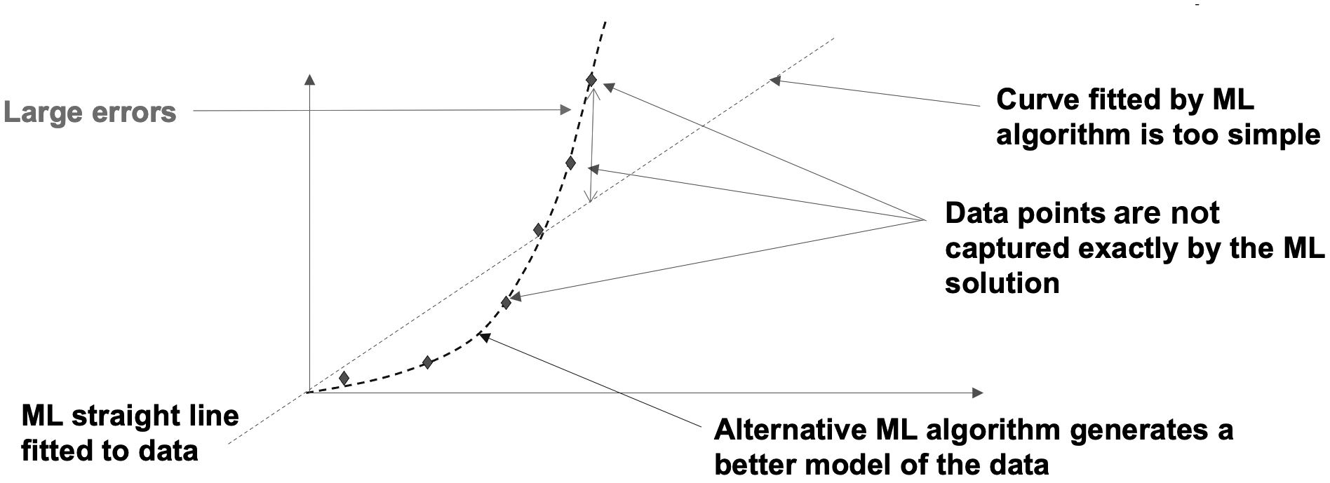
Under-fitting, on the other hand, is the opposite; it tries to fit a curve (using our simple curve idea) that is not complicated enough. In Figure 4.18 we see that our data set is well represented by a parabola (dashed line) or a second order curve. If we try to fit a simple linear straight line to the data, we again see large errors.

Figure 4.18 A simple example of under-fitting

So, our algorithm suffers from two types of error: bias error and variance error. The bias is how far your prediction is from the actual data. Variance is how scattered around our prediction is. With over-fitting, we see a high variance around and low bias with our training data. With under-fitting, we see a low variance around and high bias with our training data. The trade-off, shown graphically in Figure 4.19, minimises the error by finding the best level of complexity. This is not the only way to assess the efficacy of an algorithm. There are many other ways, and there are numerous examples to be found in the books listed in Further Reading at the end of this book. We should also note in passing that the trade-off uses test data that have not been used to train our algorithm.

Remember that the learning from experience within a ML project involves the whole team. The domain expert is the person that defines what is fit for purpose.

4.1.5 Typical methods of visualising data

Visual representation of data is one area where a focus on AI or ML can enhance how you organise and present data. The benefits of good visualisation must be a priority as, ultimately, we are judged by clients, stakeholders and/or users on the deployed AI or presentation of results. Visualisation is a fundamental enabler of learning from experience for everyone on the team. Figure 4.20 again shows the stages of a ML project and highlights how visualisation can help with learning from experience at every stage (see Géron’s eight stages in Section 4.1.2).

If we can visualise data from the start of a project, we magnify our learning – a picture paints a thousand words. In addition, we are already organising our data so we can manage them and use them. If we are in a highly regulated profession, then early engagement with stakeholders and regulators might aid the acceptance of work and results.

Figure 4.19 Algorithm assessment, the trade-off and finding the balance between under- and over-fitting

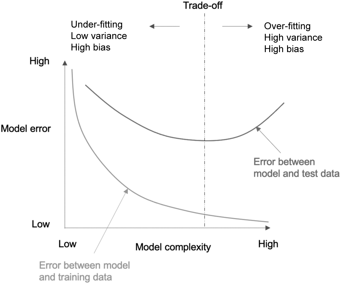
Figure 4.20 Visualisation is learning from experience at every stage of an ML project

Some typical types of data visualisation are shown in Figure 4.21. The top row are graphs of data that we might encounter in a spreadsheet. The middle row is an iso-contour plot, perhaps of the heights in a map. The image on the right-hand side is an iso-surface; from the iso-contours we can build the 3D iso-surface. With some vector calculus we can also calculate the gradients and perhaps find maximum and minimum heights. These ideas are very powerful if the data we are plotting is the learning rate of a NN or the profit from business activities. We can focus on the fast learning rate or maximise our profit. The bottom row of the examples are networks; these are more complex structures to visualise. Here techniques such as stereo vision, augmented or virtual reality can help. Even large displays such as power walls allow a different perspective on data we are presenting.

These types of data visualisation technique have been around for decades, and software on our computers enable us to create them. However, when we move to large data sets from simulations or Big Data, we need parallel data-processing capability. ParaView (https://www.paraview.org) is a parallel data visualisation ecosystem with Python at its core. It is built on the Visualization Toolkit open-source 3D graphics, image processing and visualisation software library and constructed to run on parallel computers, so can process large data sets and produce graphics that an individual user can see. This is a major challenge when working with large data sets – working with large data sets on parallel computers is not something that should be attempted on your first project.

Most laptop and desktop computers are multi-core and multi-processor machines with graphics processing units (GPUs) that have enough processing power and capability to learn and develop ML/AI. Once tested on small hardware, you can then gradually use greater processing power on high-performance computing systems.

We are fortunate that most open-source software can be compiled, or is already compiled, for common operating systems. You can initially work on your own hardware using the same software you will use on larger hardware set-ups. We are also lucky to have both open-source and commercial software we can draw on. There are advantages and disadvantages to both, and you will need to consider what you will require. A search on your favourite search engine will bring up a list of the many data visualisation packages around.

We know that visualisation is an important aid to learning from experience, but there is an additional idea that we might be able to incorporate: Can we create a learning environment? Can we develop a virtual reality (VR) or augmented reality (AR) simulated environment that we can learn from or humans can teach an AI system to learn from? We mentioned in Chapter 3 that AI robotics gives us the opportunity to explore and utilise extreme environments. Could we build simulated environments to generate the data we need to design and operate our robots? Could we build a learning environment to let a robot learn how to do a task?

Blender is open-source software with a highly sophisticated environment for building simulations and presenting data (see Figure 4.22). The graphics are capable of producing photo-realistic renderings and movies. This is often the base of computer games, movies and scientific visualisation. If we extend this to ML and AI, we could build a human and machine environment where the machine and humans interact to teach each other. Examples of this are found in engineering, where operators are taught how to operate machinery and pilots are taught how to fly in a safe environment. We are always guided by learning from experience, and the learning environment can be used to generate data.

Figure 4.21 Standard data visualisation examples: (a) line graph, (b) scatter plot, (c) histogram, (d) contour plot, (e) 3D contour plot, (f) network diagram and (g) 3D network diagram

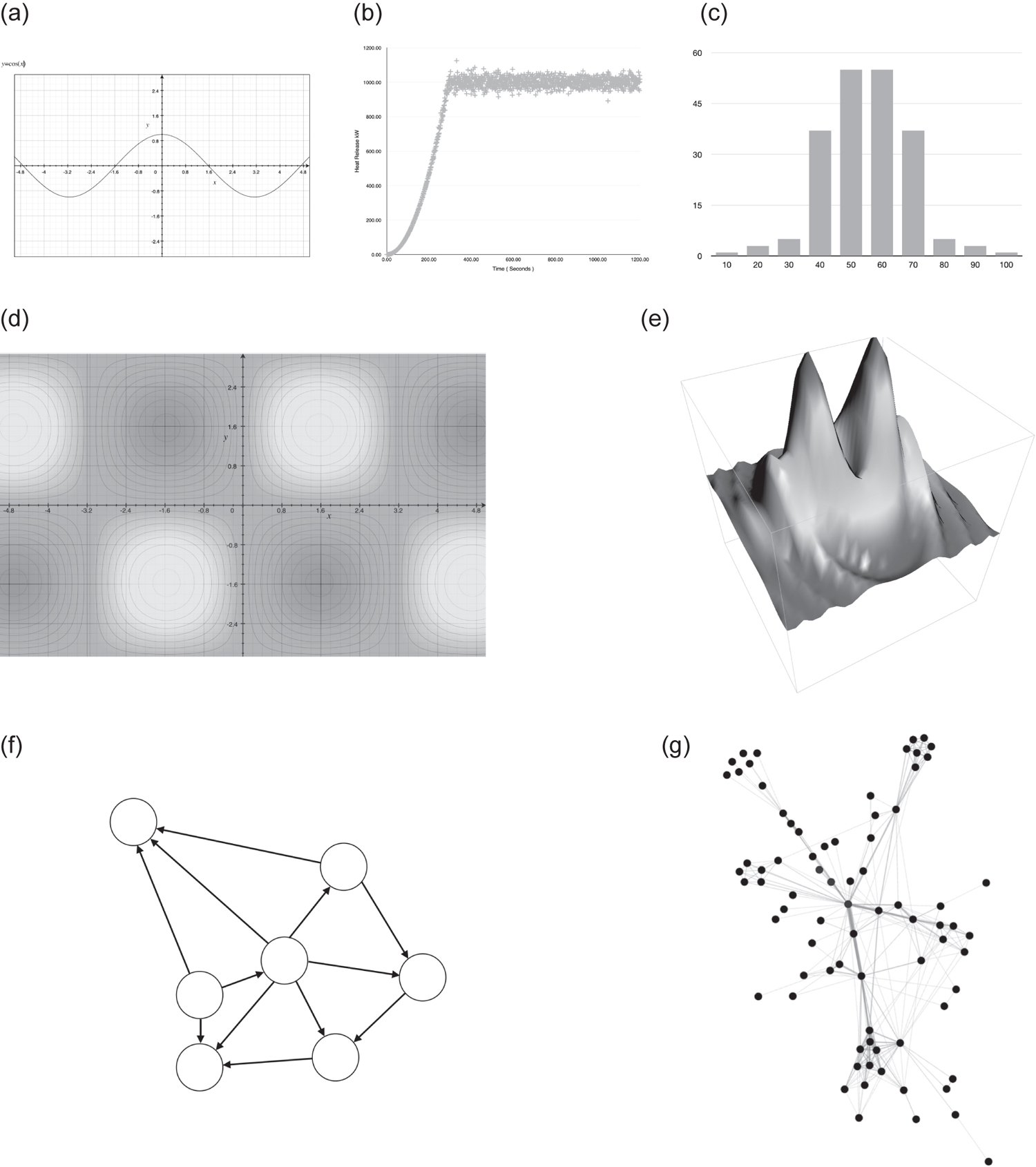
Figure 4.22 Open-source software to build simulated environments – Blender (reproduced from https://commons.wikimedia.org/wiki/File:Blender_2.90-startup.png under Wikimedia Commons licence)

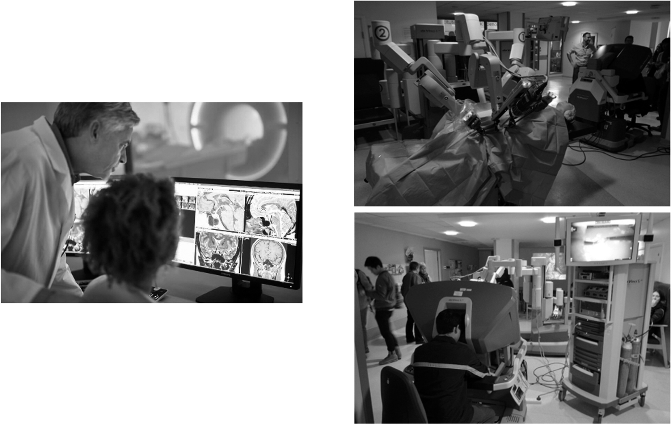
In medicine, AI can be used in diagnosis and treatment. Of particular importance in a surgical environment is what the surgeon sees. This can be developed in a digital environment first, then perhaps a physical environment and finally used on a patient. We can easily imagine a basic system, developing from scanning a patient to one where surgeons can work collaboratively with AI machines. Figure 4.23 shows examples of how AI is working in medicine from diagnosis to treatment. It shows robotic surgical equipment – the surgeon is potentially removed from the sterile operating theatre.

4.2 NEURAL NETWORKS

Here we take a closer at the neural network. In particular we describe the following:

• the link between the NN and the AI agent;
• the basic building blocks of the neural network;
• building algorithms using reinforcement learning;
• a few basic examples of what a NN can do.

Figure 4.23 AI in medicine – humans and machines working together (reproduced from (left) https://en.wikipedia.org/wiki/Radiology#/media/
File:Radiologist_interpreting_MRI.jpg; (top right) https://en.wikipedia.org/wiki/Da_Vinci_Surgical_System#/media/
File:Cmglee_Cambridge_Science_Festival_2015_da_Vinci.jpg; (bottom right) https://commons.wikimedia.org/wiki/File:Cmglee_Cambridge_
Science_Festival_2015_da_Vinci_console.jpg under Wikimedia Commons licence)

The NN gives machines the ability to learn from experience and develop their own algorithms (it is not easy to interpret what these algorithms are, as they are encoded in the NN). In recent years, our understanding on how a NN works has made significant progress. Progress includes winning complex strategy games such as chess and Go, as well as the perhaps more challenging tasks of controlling complex machinery such as robots. In doing so we are giving machines more autonomy.

There are many types of NN available to us, and one that stands out as having made a significant contribution to ML is the convolution NN. However, we are not going to go into detail about this type of NN here because the details are more complicated than the discussion we intend to have here.

To learn from problems that are complex and perhaps random (statistical), we need to use deep neural networks (DNNs). Typically, we employ DNNs for problems such as robot control, image analysis (e.g. medical images) and adversarial game playing. We will introduce what these are and why this makes training them iterative and requires specialist hardware (e.g. high-performance computers, GPUs, etc.) as we progress through the chapter. A DNN has many layers making up the NN; this is why it is called a deep NN.

4.2.1 The link between NNs and the AI agent

The NN is often shown as a sub-topic of ML (see Figure 1.1). The development of the NN started in the 1940s and is based on the biological nature of the human brain. In 1943, Warren McCulloch and Walter Pitts introduced the concept of a neuro-logical network by combining finite state machines, linear threshold decision elements and memory,⁶⁰ followed in 1947 by a paper extending these ideas to the recognition of patterns.⁶¹ The first reinforcement NN built by Marvin Minsky occurred in 1951. This was an analogue or electronic device that used reinforcement to learn.⁶² This was the start of adaptive control and we see a close link to engineering emerging. In 1962, Rosenblatt named and defined machines called Perceptrons;⁶³ however, it took until the 1980s for NN to gain significant traction. Today the theory is understood in greater depth. Digital computers have facilitated the use of convolution NN to undertake sophisticated tasks such as learning to control robots and win combinatorically complicated games.

The learning AI agent needs the ability to learn. Reinforcement DNNs or convolution NNs do just that. They can learn from sensors and actuators or from well-engineered computer simulations or games.

Narrow AI has been focused on specific problems. The NN is a more generic learning technique that can be applied to a wider range of scenarios. Training NNs is not easy and understanding their output is difficult also. This poses challenges for justifying them and using them.

4.2.2 The basic building blocks of the neural network

In this section we introduce the concept of learning that is fundamental to NNs. The Perceptron was the initial concept from which our more sophisticated NNs of today evolved. As we build up the basic building blocks of the NN, we will see how the Perceptron fits in.

The NN has a basic mathematical schematic, shown in Figure 4.24, based on the original work of McCulloch and Pitts in 1943.⁶⁰ In this figure, we also see a simple representation of a human brain neuron.

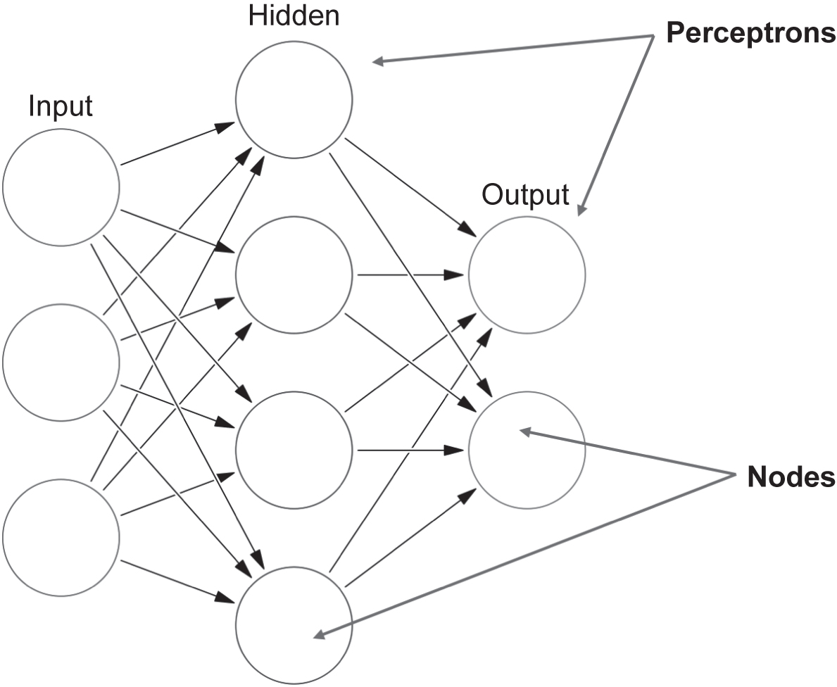
Each of these NN neurons form layers (lots of neurons), and multiple (hidden) layers make up a network. The first layer is the input layer where data are fed into the network. The data can be output from a simulation, the colour of pixels in an image or data from sensors. The data pass through the network and as they do, just like the human brain, neurons are activated (or fire). A simplified three-layer version of a NN is shown in Figure 4.25.

There can be any number of layers, and DNNs have lots of layers. Unfortunately, we do not know what number of layers, or depth of DNN, we need before we start training the NN. That is something we learn from experience as the trainer, and part of the hyper-parameters that we will systematically learn from. In this description we have been careful to use only feedforward networks where the input of the node is passed onto the next layer. Recurrent NN also allow nodes to communicate with other nodes and themselves on the same layer. These types of network are described as more dynamic and can behave chaotically. We will stick with the feedforward NNs here, as we are building an intuition or understanding.

Figure 4.24 The schematic of a neural network neuron (McCulloch and Pitts 1943) and a human brain neuron (reproduced from https://commons.wikimedia.org/wiki/File:Neuron3.png under Wikipedia Commons licence)

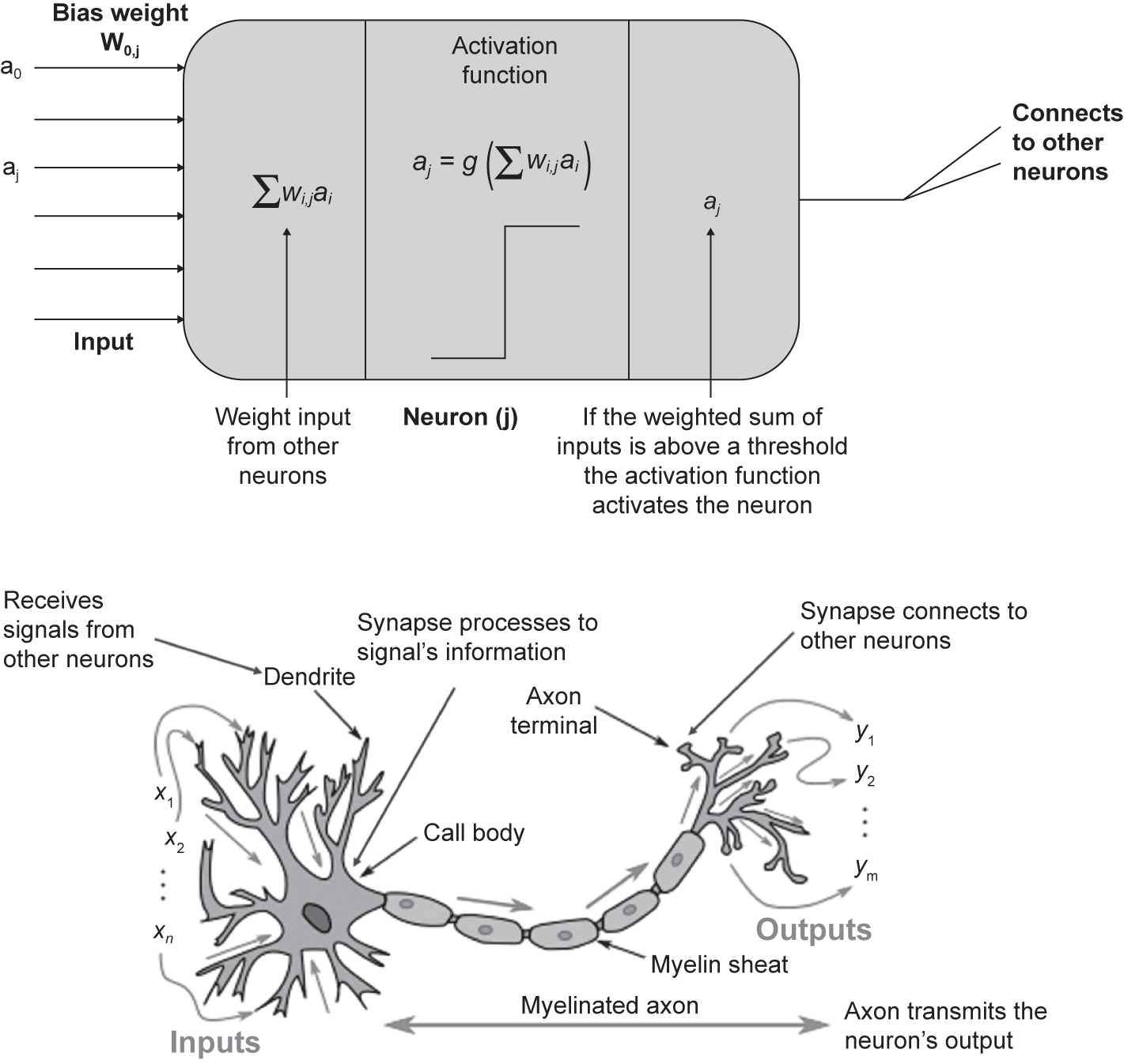
NNs work by taking the output (if it is activated) from nodes and passing this information via a link. The link connects the output of a node to nodes on the next layer. Each link from the output of a node is uniquely weighted as it is passed to other nodes. We do not know what these weights are, and training is about determining what the weights should be. An example might help here. Say we have a high resolution picture of a scene taken on your smartphone, the type of picture doesn’t matter. We can analyse this picture using a NN. The picture is held on your phone as a matrix of numbers that represent the colour of the image at a particular location. The NN takes this matrix as its input and passes this number to every node on the first layer. Before it does so, it weights it by a unique weight between the input node and the layer node it is going to. Each node on the first layer then adds up the colour number and weights it has received. This sum of weighted input colour numbers is then passed through the activation function. If the output of this operation is greater than a set value, the node is assumed to be activated and the result passed onto the next layer. If it is not activated, then this node is not activated, and its output is zero. The layer of now activated or inactivated nodes is fed into the next layer and the process is repeated. The activation function is trying to represent how our brain fires its neurons when parts of our NN are stimulated. As information is passed through the network of nodes, nodes are fired or not fired. This is a very simple analogy and training a network to find the best weights needs a bias node as well. This helps us to shift the threshold of nodes activating or not.

Figure 4.25 The schematic of a neural network with an input, hidden and output layer. In NNs, a neuron is a node in the network and the node is made up of an input and activation function and an output. Nodes are connected via links (reproduced from https://commons.wikimedia.org/wiki/File:Colored_neural_network.svg under Wikipedia Commons licence)

Whether a node is activated or not is determined by the activation function. The activation function uses the input function as its input. This input function is the sum of the output of nodes connected by the links, multiplied by the weights of the links between the nodes. We then need to determine if the node is activated. If a hard threshold (activation function output is above a set value) is used, then this is a Perceptron. These types of NN can represent non-linear problems that are Boolean in nature. The Sigmoid Perceptron uses a differentiable Sigmoid activation function, and this means DNNs can now represent arbitrary functions, again non-linear. This makes them very powerful. The threshold activation function is a hard step change between the neuron activating or not. The Sigmoid (logistic) activation function is differentiable and is called softer because the decision to fire the node is not a step change. There are other types of activation function, for which use is determined by the experience of the trainer.

The trainer needs to train the neural network to determine the unknown weights of each of the links. This is not a simple task, and a role of the future for AI personnel. Training a NN involves adjusting weights in order for the NN to improve. Techniques involve forward and back propagation to update weights based on the error between the desired output and the NN’s output. Knowledge of vector calculus will help here, and a NN domain expert will help too. Up to now we could simplify the NNs as ones that can understand functions, given examples of what those functions are. We could use a NN to learn from examples that we know. This makes the error known. What happens when we do not have labelled examples to learn from? We could build learning examples and try to form labels from our understanding of the NN.

What happens if our problem has lots of unknown combinations – such as a game with many possible moves? We simply may not have the data to understand all the possible moves. We need to measure, somehow, the performance of the NN. This is called reinforcement learning, and the NN can learn by itself. Reinforcement learning fits naturally with the learning agent schematic. The agent has a learning component and the learning component tries to maximise its reward or minimise its loss. Norvig and Russell note that reinforcement learning might be considered as encompassing all of AI.⁹ In an environment, an agent will have a percept and will learn via the learning element to achieve a goal. It will use its actuators to act on the environment. This elevates products to intelligent entities and gives products such as robots autonomy. An agent using a NN and reinforcement learning has to learn how to achieve a goal in an environment. This learning is complex. Somehow, we need to train the NN to explore its environment, create a policy to achieve a goal and understand what it can do to the environment with its actuators.

Examples of reinforcement NN successes are:

• AlphaGo, the computer that was taught to beat the world Go champion (see Section 1.3.4). The computer was so successful, it used moves that impressed Go masters. A supercomputer played itself at the game of Go to learn how to play. This is an engineered simulation environment.
• OpenAI, who used an NN to teach a robot how to solve a Rubik’s Cube.⁶⁴ The robotic hand can manipulate the cube to solve it because it has many sensors and actuators. The NN learned how to solve the Rubik Cube and also how to manipulate its environment.

4.3 AGENTS’ FUNCTIONALITY

In this section we give examples of how AI, and in particular ML, is used to give agents functionality. The functionality is used by agents to:

• interpret their precepts;
• undertake an action;
• achieve a goal.

The agent’s function is a map of how it understands its percept sequence and turns this into a goal-achieving action. This functionality is usually a high-level or abstract mathematical description of what it is doing. The physical embodiment of the AI agent is then put into the agent program that implements its functionality. Any system could be an agent, certainly from an engineering point of view. Here are some examples of the types of functionality that are useful to an agent:

• decision making;
• planning;
• optimisation;
• searching (the best option or best adversarial game options, route finding);
• natural language processing;
• representing knowledge.

When we think of computational science, engineering, operational research and the statistical and mathematical techniques available, this becomes a very long list of functionality we can build into our agents.

4.4 USING THE CLOUD – CHEAP HIGH-PERFORMANCE COMPUTING FOR AI

In this chapter we have built an understanding of the concepts and theory behind AI using ML as a guide. We can make it complicated if we are training a complex system to achieve a goal; however, once built we can use this learning over and over again. The cloud and the internet make this happen. We now have access to open-source code, improved on an international scale by experts around the world. It is usually free, and the time between academic research and practical application is reducing – progress around the world is accelerating. Software built on object orientation makes code more modular and reusable; libraries of open-source code make development slicker and more reliable. However, there comes a point when we need processing power or the ability to scale applications to a worldwide audience. Here, cloud high-performance computing comes to our aid – it is reliable and cheap (compared to building your own supercomputer).

Typical AI open-source code can be downloaded from a multitude of sources. In some cases, the code will be optimised for use on the cloud service provider’s hardware. This isn’t always necessary, as you’ll be testing and preparing your AI on a laptop or desktop. Cloud service providers also provide online training, forums and user conferences – the cloud community is collaborative.

Data security, as always, is of paramount importance, and ensuring data are protected as the law requires needs careful attention.

You will need to pay for some of the services on the cloud. When starting, there is usually a free period of time given to you for learning. This is very helpful.

4.5 SUMMARY

This chapter has built up an appreciation of the complexity of mathematics and theory that ML and AI bring to our projects. The theory of AI, ML and the subject areas it draws on are vast. With this chapter we hope to have given you an intuitive understanding of what is involved.