
There aren't many things in the world funnier than a sporty car. That's a fact.
Let's imagine we want to develop a simple cruise control system for such a car. This system will perform the following tasks:
- Read the target vehicle speed [km/h]
- Read the current vehicle speed [km/h]
- Command the throttle with the gas pedal [from 0 (not pressed) to 1 (fully pressed)]
This system will behave like a driver that keeps the car going straight using only the gas pedal to match the desired speed.
Let's get started!
After pointing MATLAB to your preferred working folder (for example, a folder called 1386EN_02 located in your home folder) and opening a new model, click on the Save button, or use the Save option under the File menu, or the Ctrl + S keyboard shortcut, and give it the name cruise_control.slx.
You'll notice that there are two file formats available. They are explained as follows:
The first format is the most widely used, but be aware that every model depends on the Simulink version used to create it; those developed with newer releases are unreadable by older releases, while newer releases can upgrade old models.
The saved model will now be visible in our working folder. If you close Simulink, you can re-open the model at a later time by dragging it to the MATLAB's Command Window.
It's always a good idea to explain what a system does. In the C programming language, you use the comment section (/* ... */) to explain a function; in Simulink, you insert a note by clicking on the Annotation tool icon (to the left of our cruise_control editor panel) or double-clicking on the white area of the model editor.
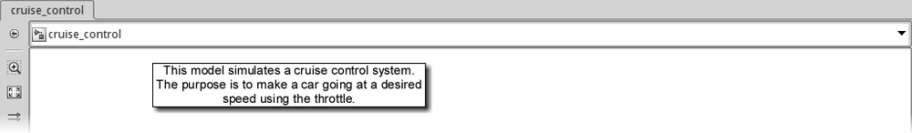
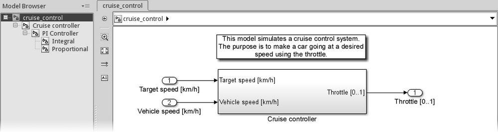
Like comments explaining functions in C, it's a good practice to insert a note at the top of the model view explaining what it does. Let's insert this note:
This model simulates a cruise control system.
The purpose is to make a car going at a desired
speed using the throttle.
By right-clicking on the note, you can set the alignment (default: centered) and draw an annotation border, to make it more eye-catching:
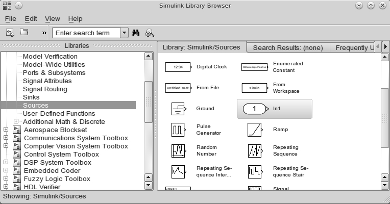
Let's start inserting some blocks from the Simulink library. We need to open the Simulink Library Browser by pressing the Library Browser button, or using the View | Library Browser menu, or using the Ctrl + Shift + L keyboard shortcut.
A new window with two panels will appear: the left panel lists all the available libraries, each one holding one or more subsets, while the right panel shows all the blocks belonging to the selected library. Block libraries are also called blocksets.
By double-clicking on a block, a new window appears with a brief block description and the parameters that the block can accept. To get detailed information about the block and how to use it, click on the Help button and the documentation center will be opened with the page describing the selected block's meaning and usage.
Navigating in the Simulink Library Browser is fairly straightforward; most of the time we'll be using blocks from the Simulink blockset (installed with the Simulink software).
The first blocks we need are input and output ports. Input ports (also called inports) are available in the Simulink | Sources blockset and are labeled In1:
Similarly, output ports are available in the Simulink | Sinks blockset and are labeled Out1.
These blocks can be placed in the model by:
Let's place one input port and one output port in the model using your preferred method.
Notice that the window title has changed and now bears an asterisk (cruise_control *). This means that the model has been edited since the last save. Save the model and the asterisk will go away.
Of course, opening the Simulink Library Browser each time you need to place a block is a tedious task and slows down development time. If a block offering the same functionality is already present in the model, you can just copy and paste it, or drag it while keeping the right mouse button pressed; a new copy will be made.
Let's add another input port by moving the mouse arrow on the previous port, and while keeping the right mouse button pressed drag it to some other position and then release the button; a small menu will appear asking you if you intend to Paste or Duplicate the port:
Notice that while dragging a block, Simulink suggests the alignment with other ports, which helps in keeping the project well-structured.
If we don't spend a little time in trying to keep the system view well organized, we'll end up with a garbled system that very much resembles the dreaded "spaghetti code" that we should avoid.
Note
A set of rules has been defined by the MathWorks Automotive Advisory Board with the automotive industry in mind. Embedded developers with code generation in mind should stick to it as closely as possible. The ruleset is available at http://www.mathworks.com/automotive/standards/maab.html.
Note that each block must have a unique name in the current subsystem. Try to rename the In2 port to In1 by double-clicking on its name; Simulink will issue an error window saying that the name already exists.
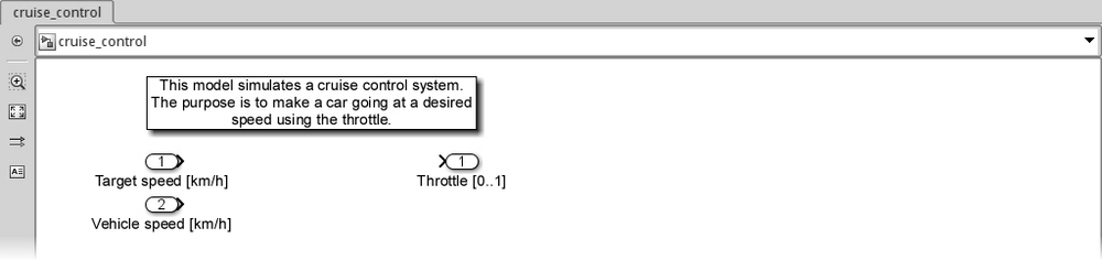
Since the labels In1 and In2 don't make a lot of sense, we'll rename them to our inputs: the Vehicle speed and the Target speed. The same goes for our output: the Throttle.
Now we should have something similar to the following screenshot:
The simplest yet most effective cruise control algorithm is a PI (Proportional-Integral) controller. This algorithm can be summarized in the following four steps:
- Calculate the error e(t), that is, the difference between the target speed and the vehicle speed.
- Apply a correction factor to the error Kp.
- Apply a correction factor to the integral of the error, Ki.
- Sum both the proportional and the integral components and obtain the control signal u(t).
The mathematical formula of a PI controller is as follows:
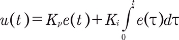
Of course, we can't push the gas pedal beyond its physical limits; the throttle control signal needs to be clamped, the lower limit being 0 (throttle closed) and the higher limit being 1 (throttle fully open).
By looking at the formula, it's easy to guess that we need to find the following blocks in the Simulink Library Browser:
- One Subtract block (from Simulink | Math Operations) in order to calculate the error
- Two Constant blocks (from Simulink | Sources) for
KpandKi, and two Product blocks (from Simulink | Math Operations) - One Integrator block (from Simulink | Continuous) used to hold the error integral
- One Add block (from Simulink | Math Operations)
- One Saturation block (from Simulink | Discontinuities) to clamp the output throttle
Note
The Integrator block (and almost every other block in the Continuous blockset) is represented with the corresponding transfer function H(s) = Y(s)/U(s) in the Laplace domain. More information can be obtained by clicking on the Help button in the block parameters window.
You don't need to know about Laplace transforms in order to understand this book; just remember that the 1/s block is an integrator.
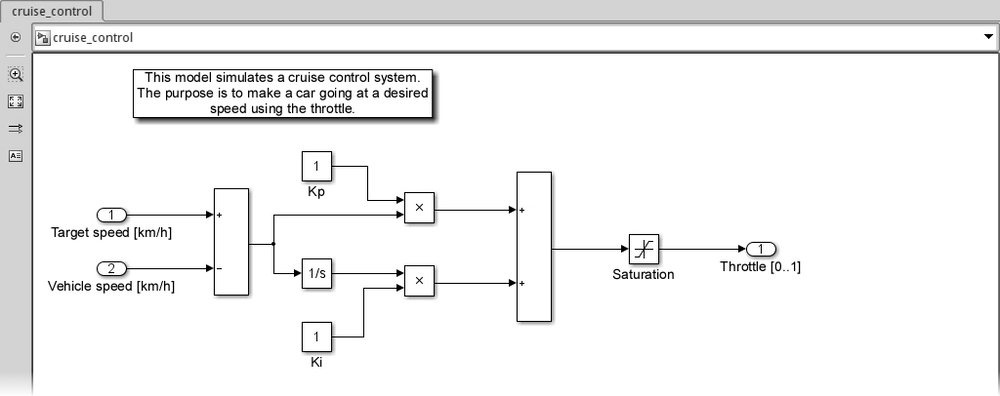
Place the blocks in the order suggested by the algorithm (refer to the following screenshot) and open every block to understand its options. Don't forget to:
- Check the Subtract block operands: the Target speed has to be connected to the positive port and the Vehicle speed to the negative port; thus the block parameter should be
+− - Edit the Saturation block limits by double-clicking on it; a window opens; in that window, set the value of Upper limit: as
1and the value of Lower limit: as0
Optionally, resize the blocks (by dragging the little handles that appear on the selected block's border), hide the math blocks' names (by right-clicking on the blocks and opening the Format submenu), and rename the constant blocks to Ki and Kp.
To connect two blocks, it's sufficient to drag the little arrow from the source block to the endpoint at the destination block with the mouse.
We should end up with a model similar to the one shown in the following screenshot:
Subsystems are a very convenient way to group together the blocks that implement a specific functionality.
In order to make a clear distinction between the PI controller components, we can select the elements to group together and right-click the selection to open the contextual menu and create a subsystem (or use the Ctrl + G keyboard shortcut). The operation is shown in the following screenshot:
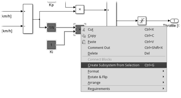
We'll create two subsystems: one for the proportional component and one for the integral component. Since they are of a small default size and have the default port names of In1 and Out1, we should resize and rename them, then open them (with a double click) and rename their ports.
We should obtain the model shown in the following screenshot:
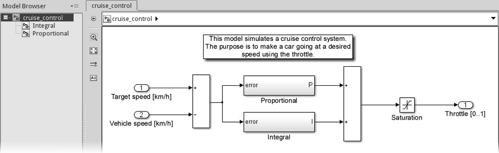
Notice the change in the Model Browser panel on the left; you can now navigate in your system hierarchy by clicking on the subsystems' names. The cruise_control block is called the root subsystem.
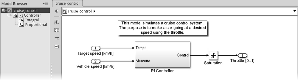
Let's continue organizing the model into subsystems by selecting all the PI controller components (everything except the ports and the Saturation block) and making a subsystem. Again, we need to edit the new subsystem's port names.
We should see the clean, ordered, neat-looking, self-explanatory system shown in the following screenshot:
The final step—the root subsystem should contain absolutely no logic, only root-level blocks implementing a complete functionality, sharing little to no signals. We still have the Saturation block left out.
So we'll select everything (literally—ports included) and create the cruise control root subsystem as shown in the following screenshot:
This time we didn't have to rename the ports; since we included them inside the selection, Simulink kept their names and created new copies outside the newly created subsystem.
There's a problem with the cruise controller; we've left the PI calibration constants inside the block, and we can't calibrate them without doing some simulations.
This means that either we dig into the model hierarchy down to the Integral and Proportional blocks every time we need to change their values, or we pull them out to the root level.
Both of these methods are viable with a simple system like the one we've just modeled. But as soon as the model complexity grows, you'll have problems either in knowing where the constants are or in having a clean, understandable system layout.
But there is a clean and effective solution. Since Simulink can read MATLAB's variables, it's easy to define the Kp and Ki constants in the MATLAB workspace and use their labels in the Constant blocks.
So we define them by entering these commands in MATLAB's Command Window:
Kp = 1;
Ki = 1;
Then we'll navigate to the constant blocks, double-click each one of them and edit the Constant Value field in their respective Source Block Parameters window with the previously defined variables Kp and Ki.
The block parameters window for Kp will look like the following screenshot:
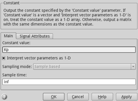
Done! Now we can edit Kp and Ki directly from the MATLAB's Command Window!
Let's save the workspace alongside the model, (that is, at the same location where cruise_control.slx is saved) calling it cruise_control.mat (click on the Save Workspace button in MATLAB's main window.).
To avoid loading it every time we open the model, we can use the PreLoadFcn model callback. Navigate to the root subsystem, right-click on the white space, and choose the Model Properties item from the contextual menu. A new window will open; click on the Callbacks tab and select the PreLoadFcn item from the list. Inside the textbox, we'll type the MATLAB command that will perform the workspace loading: load('cruise_control.mat').
To confirm that we didn't make trivial mistakes, we should run Update Diagram (from the Simulation menu or by pressing Ctrl + D).
Now we've finished our first model. It's time to see how it behaves.
Let's see how our controller works in an open loop (without actually anything to control).
We must delete the input and output ports from the root level, since we're replacing them with appropriate Sources and Sinks blocks from the Library Browser.
We'll take the following blocks from the Simulink Library Browser:
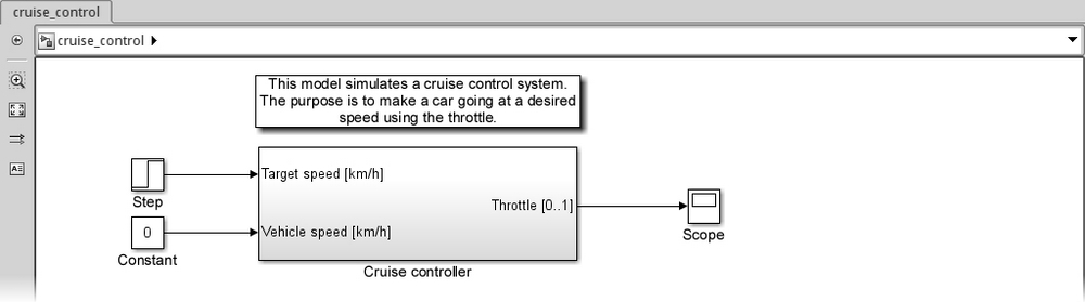
- A Constant block (from Simulink | Sources) to be connected to the Vehicle speed input with the Constant value set to
0 - A Step block (from Simulink | Sources) to be connected to the Target speed input with the Final value set to
0.1(remember that the throttle is clamped between 0 and 1) - A Scope block (from Simulink | Sinks) to be connected to the Throttle output
We should have the system looking like the following screenshot:
Running the simulation is an easy task: just click on the green Run button in the toolbar, or click the Simulation | Run menu entry, or type the Ctrl + T keyboard shortcut.
When the simulation is completed (the status bar at the bottom left shows the Ready word again), double click on the newly added Scope block and you'll see this neat graph:
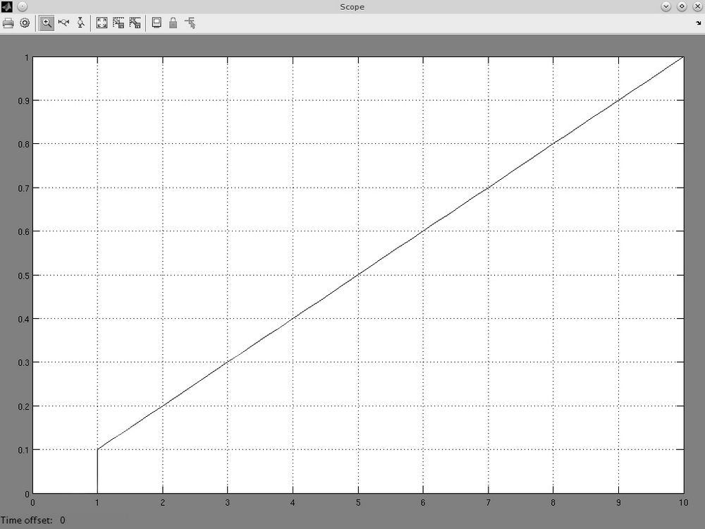
Good! Notice that the simulation stopped at the tenth second; it is the default simulation time, which can be adjusted in the Simulink toolbar (right above the model editor).
We can do our little result analysis:
- Before 1 second: the target speed is still 0, equal to the vehicle speed with no throttle required.
- At 1 second: the target speed (and the speed difference) goes to 0.1, the proportional factor of the PI controller kicks in and sets a throttle equal to the speed difference multiplied by
Kp, while the integral factor starts working. - From 1 second onwards: the proportional contribution to the throttle stays at 0.1, but the integral contribution rises linearly (
Kibeing 1, the slope of the throttle is equal to the speed difference, that is, 0.1).
Tip
A new variable has appeared in the workspace: tout. It is an array containing the time instants where the results have been calculated. By using the Sinks | To Workspace block, we can save the simulation results in the workspace too. This is often useful to do further analysis and prepare a report using MATLAB's powerful plotting functions, thus overcoming the limitations of the Scope block.
You can see that the resulting scope graph is not really continuous by opening the 'Scope' parameters window [click on the Parameters icon button (the second from the left)] and choosing a line marker (Line:) in the Style tab. Simulink automatically chose an adequate time step. We'll discuss simulation times in the next chapter.
What we have just performed is an open-loop simulation: we have a controller running without the controlled system, so the speed (or better: the error e(t) that the controller is reacting to) is made up with a Step block. The purpose of open-loop simulations is to demonstrate and check the controller behavior with certain kinds of inputs.
What now? We need a mathematical model of a controlled system in order to perform a closed-loop simulation and see how our cruise controller is able to make the speed difference disappear by commanding the throttle. We need to model a car.
Tip
Downloading the example code
You can download the example code files for all Packt books you have purchased from your account at http://www.packtpub.com. If you purchased this book elsewhere, you can visit http://www.packtpub.com/support and register to have the files e-mailed directly to you.