
We'll develop the simplest possible S-functions to enable our models to communicate with the application we described earlier: a file-source block and a file-sink block.
These S-functions will have only one port and be able to read/write a scalar real signal from/to a file. The file path will be passed as a parameter; and the files will have only one line containing the new signal value.
The sink block, called filesink_msfun, will receive the input and convert it to a string that will be written to the file. The file path is passed as parameter, no DWork vector is needed because we don't have to output a default value.
The source block, called filesource_msfun, will read one line from the file, attempt to convert it into a real number, and output it. When the file is not readable, the last line is empty, or an error occurs, the last valid value will be used. This means that we'll have to use one DWork vector, and one more parameter for the initial output.
In the following paragraphs we will walk through a detailed description of their implementation, beginning with the simpler one, the filesink_msfun block.
This block has the purpose of writing the input signal to a text file. Since the text file will be read by the external application, we can't open it once the simulation starts and close it when the simulation ends; otherwise, the application may have problems in reading it. Therefore, the file has to be opened and closed at each time step, in the Outputs callback.
Let's open an empty model and save it as msfun_test.slx.
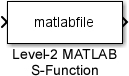
We'll immediately place the Level-2 MATLAB S-Function block from the Simulink | User-Defined Functions blockset in our model:
Double-clicking on the block will open the usual parameters window, where we need to replace the S-function name parameter with filesink_msfun:
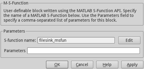
Let's click on the Edit button; since the filesink_msfun.m script file does not exist yet, Simulink will ask if we want to open the editor or locate the file. Choose the Open editor option to launch the MATLAB editor with an empty file, which we'll immediately save as filesink_msfun.m.
Tip
A quick note to Linux users: the editor is using Emacs-like shortcuts by default (for example, Ctrl + W/Ctrl + Y to copy/paste). If you're not using Emacs, you may want to switch to Windows-like shortcuts (for example, Ctrl + C/Ctrl + V to copy/paste) by opening the Preferences window and navigating to Keyboard | Shortcuts. The first item, Active settings, will let you choose between Emacs or Windows behavior.
First and foremost, we need to define the S-function entry point, that is, a function with the same name as the script file itself (minus the extension), calling the mandatory setup callback.
%% S-function entry point
function filesink_msfun(block)
setup(block);
When Simulink updates or simulates the model, it will call filesink_msfun, passing as argument one Simulink.MSFcnRunTimeBlock object containing every data about the block itself. This will, in turn, run the setup callback.
The second function we must implement is the setup callback:
%% First required callback: setup
function setup(block)
The first line in this snippet of code is a comment, followed by the function definition taking the block object as argument.
Let's set the simplest block properties first: the number of parameters, input ports, and output ports.
block.NumDialogPrms  = 1; % Number of parameters
block.NumInputPorts  = 1; % Number of inports
block.NumOutputPorts = 0; % Number of outports
In order to edit them, it's sufficient to assign the desired values to the block object's attributes. In this case, we specify that the S-function will accept only one parameter. Being a sink block, it has one input port and no output port.
We must now configure the input port:
% Set input port properties as inheritedblock.SetPreCompInpPortInfoToDynamic;

% Override some properties: scalar real input
block.InputPort(1).Dimensions = 1;
block.InputPort(1).DatatypeID = 0; % double
block.InputPort(1).Complexity = 'Real';
block.InputPort(1).SamplingMode = 'Inherited';
block.InputPort(1).DirectFeedthrough = 1;
We begin by initializing the first input port properties (dimensions, datatype, complexity, and sampling mode) to be inherited from the driving block. Remember that the elements in a vector are accessed with one-based indexes.
Then we explicitly set the properties to make the input port a one-dimensional double-precision real number. The sampling mode is set as inherited from the previous block, but (unless you have the DSP System ToolboxTM product installed) the only possible value is Sample. Finally we set the DirectFeedthrough property in order to execute this block after the driving one.
Since we don't have to configure any output port, we proceed by defining the sample times:
% Set the sample time and the offset time.
%  [0 offset]            : Continuous sample time
%  [positive_num offset] : Discrete sample time
%  [-1, 0]               : Inherited sample time
%  [-2, 0]               : Variable sample time
block.SampleTimes = [-1 0];
This parameter accepts a vector: the first element is the sampling time period and the second is the initial offset time (both are expressed in seconds).
The possible combinations are as follows:
[0 Y]: For a continuous sample time withYoffset, meaning that a new sample will be acquired every time step[X Y]: For a discrete sampling period ofXseconds withYoffset[-1 0]: To inherit the sample time from the driving block[-2 0]: To declare a variable sample time, useful only with variable-step solvers
Here we set the sample time as inherited from the driving block (-1). This block will be executed immediately after the driving one.
The next step is to define how this block should behave when the user tries to save or restore a simulation state:
% Specify the block simStateCompliance. The allowed values are:
%    'UnknownSimState', < The default setting; warn and assume DefaultSimState
%    'DefaultSimState', < Same sim state as a built-in block
%    'HasNoSimState',   < No sim state
%    'CustomSimState',  < Has GetSimState and SetSimState methods
%    'DisallowSimState' < Error out when saving or restoring the model sim state
block.SimStateCompliance = 'HasNoSimState';
Since this block, not having a DWork vector, has no simulation state to save or restore, we use the 'HasNoSimState' constant. Another valid option would have been 'DefaultSimState', which would end up doing nothing anyway.
Tip
To understand what a simulation state is, and when it could be useful, refer to this page in the Documentation center: Simulink | Simulation | Run Simulation | Interactive | Save and Restore Simulation State as SimState.
The default setting is 'UnknownSimState', which is equivalent to 'DefaultSimState', with a warning issued when the user attempts to save or restore the simulation state.
Now every block property has been defined and Simulink should be theoretically able to do a model update. But there's one information missing to complete the initialization phase. We have to register every other implemented callback at the end of the setup function.
Since we'll need the mandatory Outputs callback, we'll register it now:
block.RegBlockMethod('Outputs', @Outputs); % RequiredThe RegBlockMethod function tells Simulink that the required callback ('Outputs') is implemented by another function (@Outputs). We could have called that function Foo and used block.RegBlockMethod('Outputs', @Foo)to register it. It's not mandatory to use the same name as the callback, but it's always better to keep things simple.
The final step is to implement the Outputs function's required callback:
%% Second required callback: Outputs
function Outputs(block)
% open the file as write-only
fid = fopen(block.DialogPrm(1).Data, 'w'),
% print input port value to file
fprintf(fid, '%f', block.InputPort(1).Data);
% close the file
fclose(fid);
We're retrieving the value of the first parameter from the DialogPrm vector: it contains the filename.
The file is then opened in write mode using fopen, which returns the file identifier stored in fid.
fprintf will print to the file pointed by fid one line, that is, the number in fixed-point notation. This number is the signal we got from the first input port (accessed the same way as the parameter).
Finally, we're closing the file with fclose.
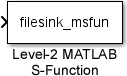
The script is complete. Save the filesink_msfun.m script and close the S-function block properties dialog window. You'll notice that the block appearance has changed, the output port has disappeared, and the script filename is shown without the extension:
Let's develop the corresponding source block now.
The filesource_msfun block has the purpose of reading its output signal from a text file, passed as parameter. Like we discussed before, the file can't be left open since the external application will be using it too. Therefore, we have to open and close the file at each time step.
Moreover, we have to provide a fallback value if the file isn't readable. That fallback will be the last valid value stored in a DWork vector. An initial value needs to be set via another parameter.
Repeating the same steps seen above, we add another Level-2 MATLAB S-function to the msfun_test.slx model, and start developing the new script that will be called filesource_msfun.m.
The S-function entry point, as we saw before, must have the same name as the file and must execute the setup callback:
%% S-function entry point
function filesource_msfun(block)
setup(block);
The mandatory setup callback will define the block characteristics, telling Simulink there are two parameters and one scalar, real output:
%% First required callback: setup
function setup(block)
block.NumDialogPrms  = 2; % Number of parameters
block.NumInputPorts  = 0; % Number of inports
block.NumOutputPorts = 1; % Number of outports

% Set the default properties to all ports
block.SetPreCompPortInfoToDefaults;
This time we won't inherit the port characteristics from other blocks; we will just set the default options.
% Set the sample time and the offset time.
block.SampleTimes = [0 0];
The same applies to the sample time. We want the block to be run at each time step, so we're using the continuous sample time option with zero offset time.
% Specify the block simStateCompliance.
block.SimStateCompliance = 'DefaultSimState';
This block will have one DWork vector. By using 'DefaultSimState', we'll instruct Simulink to save it into the simulation state.
Since we're using a DWork vector, we must register the optional callbacks (PostPropagationSetup) to define it, set its initial value (Start), and perform its update (Update) after the outputs have been calculated:
block.RegBlockMethod('PostPropagationSetup',@PostPropagationSetup);
block.RegBlockMethod('Start', @Start);
block.RegBlockMethod('Outputs', @Outputs); % Required
block.RegBlockMethod('Update', @Update);
Now we have to implement the callbacks, using the same order Simulink will call them with.
The first callback is the one that sets the DWork vector properties:
%% First optional callback: PostPropagationSetup
function PostPropagationSetup(block)
We must define how many DWork vectors we need. Since the variable that we need to store is the last valid output and there's only one output port, we need only one DWork vector:
block.NumDworks = 1;
block.Dwork(1).Name = 'lastValue'; % required!
block.Dwork(1).Dimensions = 1;
block.Dwork(1).DatatypeID = 0; % double
block.Dwork(1).Complexity = 'Real';
block.Dwork(1).Usage = 'DWork';
That vector is accessed using a one-based index. We define the vector to be one-dimensional, able to store a double datatype representing a real number. We're not interested in logging facilities, so we use the generic usage type 'DWork' (that is the default, so we could safely omit it).
The DWork vector has to be initialized before the simulation loop; this is done with the Start callback:
%% Second optional callback: Start
function Start(block)
block.Dwork(1).Data = block.DialogPrm(2).Data;
We just store the second parameter, which holds the initial output, inside the first DWork vector data.
The other required callback, Outputs, implements the logic that reads the source file:
%% Second required callback: Outputs
function Outputs(block)
% open file as readonly
fid = fopen(block.DialogPrm(1).Data, 'r'),
% read one line
tline = fgetl(fid);
if (tline == -1) % fail
    % output last value
    block.OutputPort(1).Data = block.Dwork(1).Data;
    return
end
% convert to double
output = str2double(tline);
% check that the output is a valid number
if (isnan(output)) % fail
    % output last value
    block.OutputPort(1).Data = block.Dwork(1).Data;
    return
end
% output the read value
block.OutputPort(1).Data = output;
fclose(fid);
The file, whose path is the first parameter of the S-function, is opened in read-only mode with fopen. The fgetl function will attempt to read a line from the file. If the line is valid, the str2double function will parse it, putting the result into the output variable. If that variable actually contains a valid number, it is sent to the first output port. Finally the file is closed with fclose.
If something fails, the number stored in the first DWork vector will be sent instead, and the file is closed.
The final Update callback, called immediately after the Outputs callback, is the one that will update the DWork vector with the last output value:
%% Third optional callback: Update
function Update(block)
block.Dwork(1).Data = block.OutputPort(1).Data;
We're now done. Save the filesource_msfun.m script and check that the S-function block changes, having only the output port and displaying the new S-function name.
To check that everything is working, let's add to the msfun_test.slx model a Sine wave, a Mux, and a Scope. Connect the blocks as shown in the following screenshot:
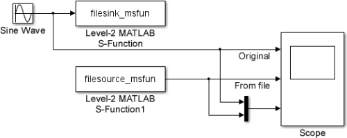
Set the filesource_msfun parameter to 'testfile' 0, and the filesink_msfun parameter to 'testfile' (don't forget the single quotation marks around the filename), then set the Fixed-Step Discrete solver with a time step of 0.1 seconds in the Model configuration parameters window (Ctrl + E) and run the simulation.
By double-clicking on the Scope block we should see the following result:
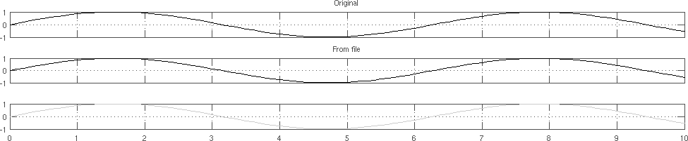
Good! The S-functions are working as expected: the filesink_msfun block has created the file named testfile in the workspace and written the Sine wave signal output to it. Meanwhile, the filesource_msfun is reading the value from the same file. A comparison of the two waves, shown in the third graph, shows that they are coincident.
Note
If we changed the direct feedthrough setting of the filesink_msfun block input to 0, we would see the second wave being late by 0.1 seconds. This is because Simulink will not know that the Sine Wave block must be executed before the filesink_msfun block.
The block execution order can be viewed in the model window by selecting the Display | Blocks | Sorted Execution Order menu item.